Autofeedback scheme for preservation of macroscopic coherence
in microwave cavities

Abstract

We present a scheme for controlling the decoherence of a linear superposition of two coherent states with opposite phases in a high-Q microwave cavity, based on the injection of appropriately prepared “probe” and “feedback” Rydberg atoms, improving the one presented in [D. Vitali et al., Phys. Rev. Lett. 79, 2442 (1997)]. In the present scheme, the information transmission from the probe to the feedback atom is directly mediated by a second auxiliary cavity. The detection efficiency for the probe atom is no longer a critical parameter, and the decoherence time of the superposition state can be significantly increased using presently available technology.

I Introduction

The problem of how the classical macroscopic world emerges from the quantum substrate is an important point in the interpretation of quantum mechanics and it is still the subject of an intense debate [1, 2]. This problem is well illustrated by the possibility, opened by quantum mechanics, of having linear superpositions of macroscopically distinguishable states, the so-called “Schrödinger cat” states. An explanation of why we never observe these paradoxical states is proposed by the decoherence models, i.e., the rapid transformation of these linear superpositions into the corresponding classical statistical mixture, caused by the unavoidable entanglement of the system with uncontrolled degrees of freedom of the environment [1]. The decoherence time depends on the form of system-environment interaction [3] but, in most cases, it is inversely proportional to the squared “distance” between the two states of the superposition [4]. For macroscopically distinguishable states, the decoherence process becomes thus practically instantaneous [1]. Decoherence is experimentally accessible only in the mesoscopic domain. In this case, one is able to monitor the progressive emergence of classical properties from the quantum ones. A first important achievement has been obtained by Monroe et al. [5], who prepared a trapped ${\rm{}^{9}Be^{+}}$ ion in a superposition of spatially separated coherent states and detected the quantum coherence between the two localized states. However, the decoherence of the superposition state has not been studied in this experiment. The progressive decoherence of a mesoscopic Schrödinger cat has been observed for the first time in the experiment of Brune et al. [6], where the linear superposition of two coherent states of the electromagnetic field in a cavity with classically distinct phases has been generated and detected.

With the impressive development of quantum information theory in the last years [7], the study of decoherence has become important not only from a fundamental, but also from a more practical point of view. All the quantum information processing applications rely on the possibility of performing unitary transformations on a system of $N$ quantum bits, whose decoherence has to be made as small as possible. For this reason, decoherence control is now a rapidly expanding field of investigation. In this respect, quantum error correction codes [8] have been developed in which the entangled superposition state of $N$ qubits is “encoded” in a larger number of qubits. Assuming that only a fraction of qubits decoheres, it is then possible to reconstruct the original state with a suitable decoding procedure, provided that errors affect different qubits independently. These codes always require the entanglement of a large number of qubits, and will become practical only if quantum networks of tens of qubits become available. Up to now, the polarization states of three photons have been entangled at most [9]. Entangled states of two Rydberg atoms [10] or of two trapped ions [11] at most can be generated. Therefore, in the present experimental situation, it is more realistic to study complementary and more “physical” ways to harness decoherence, based on the knowledge of the specific process causing decoherence, which could be applied with very few degrees of freedom. This is possible, in particular, in quantum optics, when information is encoded in the quantum states of an electromagnetic mode (see for example [12]). In this case decoherence is caused by photon leakage. It could therefore be possible to develop experimental schemes able to face photon leakage and the associated decoherence.

A series of papers [13, 14, 15, 16, 17] have shown that a possible way to control decoherence in optical cavities is given by appropriately designed feedback schemes. Refs. [13] show that a feedback scheme based on the continuous homodyne measurement of an optical cavity mode is able to increase the decoherence time of a Schrödinger cat state. In Ref. [16, 17] a feedback scheme based on continuous photodetection and the injection of appropriately prepared atoms has been considered. This scheme, in the limit of very good detection efficiency, is able to obtain a significant “protection” of a generic quantum state in a cavity. In [15, 17] this photodetection-mediated scheme has been adapted to the microwave experiment of Ref. [6] in which photodetectors cannot be used. The cavity state can only be indirectly inferred from measurements performed on probe atoms which have interacted with the cavity mode. Under ideal conditions, this adaptation to the microwave cavity case leads to a significant increase of the lifetime of the Schrödinger cat generated in [6]. It suffers however from two important limitations, making it very inefficient when applied under the actual experimental situation. It first requires the preparation of samples containing exactly one Rydberg atom sent through the apparatus. Up to now, the experimental techniques allow only to prepare a sample containing a random atom number, with a Poisson statistics. Two-atom events are excluded only at the expense of a low average atom number, lengthening the feedback loop cycletime [10]. The original scheme requires also a near unity atomic detection efficiency, which is extremely difficult to achieve even with the foreseeable improvements of the experimental apparatus.

In this paper we present a significant improvement of the microwave feedback scheme described in [15, 17]. This new version, using a direct transmission of the quantum information from the probe to the feedback atom, does not require a large detection efficiency, removing one of the main difficulties of the previous design. It however also requires sub-poissonian atom statistics. We show briefly how such atomic packets could be in principle prepared with standard laser techniques. Finally, our scheme improves the efficiency of the feedback photon injection in the cavity by using an adiabatic rapid passage.

The paper is organized as follows: in section II the feedback scheme of [15, 17] is reviewed and critically discussed; in section III the modifications of this scheme are introduced and in section IV the map describing the feedback cycle is derived. In section V the dynamics in the presence of feedback is studied and the protection capabilities of the new proposal are illustrated, while section VI is devoted to concluding remarks.

II The feedback scheme based on atomic detection

Let us briefly review the original “stroboscopic” feedback scheme for microwave cavities proposed in [15, 17]. This proposal is based on a very simple idea: whenever the cavity looses a photon, a feedback loop supplies the cavity mode with another photon, through the injection of an appropriately prepared atom. However, since there are no good enough photodetectors for microwaves, one has to find an indirect way to check if the high-Q microwave cavity has lost a photon or not. In the experiment of Brune et al. [6], information on the cavity field state is obtained by detecting the state of a circular Rydberg atom which has dispersively interacted with the superconducting microwave cavity. This provides an “instantaneous” measurement of the cavity field and suggests that continuous photodetection can be replaced by a series of repeated measurements, performed by non–resonant atoms regularly crossing the high-Q cavity, separated by a time interval $\tau_{pr}$.

The experimental scheme of the stroboscopic feedback loop is a simple modification of the scheme employed in Ref. [6]. The relevant levels of the velocity-selected atoms are two adjacent circular Rydberg states with principal quantum numbers $n=50$ and $n=51$ (denoted by $|g\rangle$ and $|e\rangle$ respectively) and a very long lifetime ($30$ ms). The high-Q superconducting cavity is sandwiched between two low-Q cavities $R_{1}$ and $R_{2}$, in which classical microwave fields resonant with the transition between $|e\rangle$ and $|g\rangle$ can be applied.

The high-Q cavity $C$ is instead slightly off-resonance with respect to the $e\,\rightarrow\,g$ transition, with a detuning

$$\delta=\omega-\omega_{eg}\;,$$ (1)

where $\omega$ is the cavity mode frequency and $\omega_{eg}=(E_{e}-E_{g})/\hbar$. The Hamiltonian of the atom-microwave cavity mode system is the usual Jaynes-Cummings Hamiltonian, given by

$$H_{JC}=E_{e}|e\rangle\langle e|+E_{g}|g\rangle\langle g|+\hbar\omega a^{\dagger}a$$ (2)

$$+\hbar\Omega\left(|e\rangle\langle g|a+|g\rangle\langle e|a^{\dagger}\right)\;,$$ (3)

where $\Omega$ is the vacuum Rabi coupling between the atomic dipole on the $e\,\rightarrow\,g$ transition and the cavity mode. In the off-resonant case and perturbative limit $\Omega\ll\delta$, the Hamiltonian (3) (under an appropriate redefinition of level phases) assumes the dispersive form [17, 18, 19]

$$H_{disp}=\hbar\frac{\Omega^{2}}{\delta}\left(|g\rangle\langle g|a^{\dagger}a-|e\rangle\langle e|a^{\dagger}a\right)\;.$$ (4)

The Schrödinger cat state is generated when the cavity mode is initially in a coherent state $|\alpha\rangle$ and the Rydberg atom, which is initially prepared in the state $|e\rangle$, is subjected to a $\pi/2$ pulse both in $R_{1}$ and in $R_{2}$. In fact, when the atom has left the cavity $R_{2}$, the joint state of the atom-cavity system becomes the entangled state [6, 17, 19]

$$|\psi_{atom+field}\rangle=\frac{1}{\sqrt{2}}\left(|e\rangle\left(|\alpha e^{i\phi}\rangle-|\alpha e^{-i\phi}\right)+|g\rangle\left(|\alpha e^{i\phi}\rangle+|\alpha e^{-i\phi}\right)\right)\;,$$ (5)

where $\phi=\Omega^{2}t_{int}/\delta$ and $t_{int}$ is the interaction time in $C$. A cat state, i.e. a linear superposition of two coherent states with different phases, is then conditionally generated in the microwave cavity as soon as one of the two circular atomic states is detected.

As it was shown in Ref. [17], the stroboscopic feedback scheme works only for Schrödinger cat states with a definite parity, i.e. even or odd cat states, and therefore we shall restrict to $\phi=\pi/2$ from now on. In fact, when the cavity field initial state is a generic density matrix $\rho$, the state of the probe atom-field system after the two $\pi/2$ pulses and the $\phi=\pi/2$ conditional phase-shift can be written as [17]

$$\rho_{atom+field}=|e\rangle\langle e|\otimes\rho_{e}+|g\rangle\langle g|\otimes\rho_{g}+|e\rangle\langle g|\otimes\rho_{+}+|g\rangle\langle e|\otimes\rho_{-}\;,$$ (6)

where

$$\rho_{e} = P_{odd}\rho P_{odd}$$ (7)

$$\rho_{g} = P_{even}\rho P_{even}\;,$$ (8)

are the projections of the cavity field state onto the subspace with an odd and even number of photons, respectively, and the operators $\rho_{\pm}$ (whose expression is not relevant here) are given in [17]. Eq. (6) shows that there is a perfect correlation between the atomic state and the cavity field parity, which is the first step in an optimal quantum non demolition measurement of the photon number [20]. It is possible to prove that this perfect correlation between the atomic state and a cavity mode property holds only in the case of an exact $\phi=\pi/2$-phase shift sandwiched by two classical $\pi/2$ pulses in cavities $R_{1}$ and $R_{2}$ [17]. Moreover, the entangled state of Eq. (6) allows to understand how it is possible to check if the microwave cavity $C$ has lost a photon or not and therefore to trigger the feedback loop, using atomic state detection only. The detection of $e$ or $g$ determines the parity of the field and, provided that the probe atomic pulses are frequent enough, indicates whether a microwave photon has left $C$ or not. In fact, let us consider for example the case in which an odd cat state is generated (first atom detected in $e$): a probe atom detected in state $e$ means that the cavity field has remained in the odd subspace. The cavity has therefore lost an even number of photons. If the time interval $\tau_{pr}$ between the two atomic pulses is much smaller than the cavity decay time $\gamma^{-1}$, $\gamma\tau_{pr}\ll 1$, the probability of loosing two or more photons is negligible and this detection of the probe atom in $e$ means that no photon has leaked out from the high-Q cavity $C$. On the contrary, when the probe atom is detected in $g$, the cavity mode state is projected into the even subspace. The cavity has then lost an odd number of photons. Again, in the limit of enough closely spaced sequence of probe atoms, $\gamma\tau_{pr}\ll 1$, the probability of loosing three or more photons is negligible. A detection in $g$ means that one photon has exited the cavity. Therefore, for achieving a good protection of the initial odd cat state, the feedback loop has to supply the superconducting cavity with a photon whenever the probe atom is detected in $g$, while feedback must not act when the atom is detected in the $e$ state.

In Ref. [17] it has been proposed to realize this feedback loop with a switch connecting the $g$ state field-ionization detector with a second atomic injector, sending an atom in the excited state $e$ into the high-Q cavity. The feedback atom is put in resonance with the cavity mode by another switch turning on an electric field in the cavity $C$ when the atom enters it, so that the level $e$ is Stark-shifted into resonance with the cavity mode.

As it is shown in Ref. [17], if the probe atomic pulses are sufficiently frequent, this stroboscopic feedback scheme becomes extremely efficient and one gets a good preservation of an initial Schrödinger cat state. However, if we consider the adaptation of this scheme to the present experimental apparatus of Ref. [6], we see that it suffers from two main limitations, which significantly decrease its efficiency. First of all the scheme is limited by the non-unit efficiency of the atomic state detectors ($\eta_{det}\simeq 0.4$), since the feedback loop is triggered only when the $g$-detector clicks. Most importantly, the above scheme assumes one has perfect “atomic guns”, i.e. the possibility of having probe and feedback atomic pulses with exactly one atom. This is not experimentally achieved up to now. The actual experiment [6] has been performed using atomic pulses with a probability of having exactly one atom $p_{1}\simeq 0.2$, close to the mean atom number in the sample. This low mean atom number has been chosen to minimize two–atom events. In this experimental situation, the proposed stroboscopic feedback scheme would have an effective efficiency $\eta_{eff}=\eta_{det}p_{1}^{2}\simeq 0.016$, too low to get an appreciable protection of the Schrödinger cat state. We show here how this scheme may be improved and adapted to the experimental apparatus employed in Ref. [6].

III The new stroboscopic feedback loop

The limitations due to the non-unit efficiency of the atomic detectors could be avoided if we eliminate the measurement step in the feedback loop and replace it with an “automatized” mechanism preparing the correct feedback atom whenever needed. This mechanism can be provided by an appropriate conditional quantum dynamics. We need a “controlled-NOT” gate between the probe atom and the feedback atom, because the feedback atom has to remain in an “off”state if the probe atom exits the cavity of interest $C$ in the $e$ state, while the feedback atom has to be in the excited state $e$ when the probe atom leaves $C$ in the $g$ state (we are still assuming the initial generation of an odd cat state). This conditional dynamics can be provided by a second high-Q microwave cavity $C^{\prime}$, similar to $C$, replacing the atomic detectors, crossed by the probe atom first and by the feedback atom soon later. A schematic description of the new feedback scheme, with the second cavity $C^{\prime}$ replacing the atomic state detectors is given by Fig. 1.

The cavity $C^{\prime}$ is resonant with the transition between an auxiliary circular state $i$, which can be taken as the immediately lower circular Rydberg state $n=49$, and level $g$. The interaction times have to be set so that both the probe and the feedback atom experience a $\pi$ pulse when they cross the empty cavity $C^{\prime}$ in state $g$ (or when they enter in state $i$ with one photon in $C^{\prime}$). This interaction copies the state of the probe atom onto the cavity mode and back onto the feedback atom. $C^{\prime}$ acts thus as a “quantum memory” [21], transferring directly the quantum information between the two atoms without need of a detection. This removes thus any need for a unit detection efficiency.

This fine tuning of the interaction times to achieve the $\pi$–spontaneous emission pulse condition can be obtained applying through the superconducting mirrors of $C^{\prime}$ appropriately shaped Stark-shift electric fields which puts the atoms in resonance with the cavity mode in $C^{\prime}$ only for the desired time. In this way, since $C^{\prime}$ is initially in the vacuum state, one has

$$|e\rangle_{p}|0\rangle_{C^{\prime}} \rightarrow |e\rangle_{p}|0\rangle_{C^{\prime}}$$ (9)

$$|g\rangle_{p}|0\rangle_{C^{\prime}} \rightarrow |i\rangle_{p}|1\rangle_{C^{\prime}}$$ (10)

when the probe atom crosses $C^{\prime}$; soon later a feedback atom enters $C^{\prime}$ in the state $|i\rangle_{f}$ and one has

$$|i\rangle_{f}|0\rangle_{C^{\prime}} \rightarrow |i\rangle_{f}|0\rangle_{C^{\prime}}$$ (11)

$$|i\rangle_{f}|1\rangle_{C^{\prime}} \rightarrow |g\rangle_{f}|0\rangle_{C^{\prime}}$$ (12)

(the cavity has a very high Q and therefore the probability of photon leakage in the meanwhile is negligible). In this way the cavity $C^{\prime}$ is always left disentangled in the vacuum state. The feedback atom exiting $C^{\prime}$ in $|g\rangle$ can be promoted to $|e\rangle$ before entering $C$, as required by the feedback scheme, by subjecting it to a $\pi$ pulse in the classical cavity $R_{2}$ (see Fig. 1). The conditional dynamics provided by $C^{\prime}$ eliminates any limitation associated to the measurement and leads to an “automatic feedback” scheme with unit efficiency in principle.

As mentioned above, an important limitation of the stroboscopic feedback scheme of [15, 17] is that it requires exactly one probe and one feedback atom per loop. This condition is still needed in the new scheme with the cavity $C^{\prime}$ replacing the atomic detectors. With two or more probe atoms simultaneously in $C$ and in $C^{\prime}$, one gets a wrong phase shift for the field in $C$ and also an incomplete excitation transfer from the probe atom to the field in $C^{\prime}$. The same condition holds for the feedback atoms. With two or more feedback atoms in the sample, the excitation transfers in $C^{\prime}$ and $C$ are incomplete.

A better control of the atom number, providing single atom events with a high probability, could be achieved by a modification of the Rydberg atoms preparation techniques. We outline here briefly the method, which could be implemented in a future version of the experimental set–up. The Rydberg atoms preparation would start from a very low–intensity velocity–selected Rubidium atomic beam. The ground state atom density is so low that the average distance between the atoms in the beam is of the order of a few millimeters. It means that a section of the beam a few millimeters long contains on the average only one atom (with a Poisson statistics). This section could be driven by a laser resonant on the 5S to 5P transition (see Fig. 2 for a schematic diagram of the relevant ⁸⁵Rb energy levels involved). The fluorescence signal should make it possible to distinguish easily the situations where the probed section of the beam contains zero, one, two or more atoms, implementing an atom counter. When the section contains zero, two or more atoms, it is discarded. The system waits then for a time $\tau_{pr}$ (a few microseconds to twenty microseconds, depending upon the atomic velocity and the precise length of the atomic beam section) until a fresh section of the beam comes in the probe laser beam. At variance, if the fluorescence level corresponds to exactly one atom, the circular state preparation is started. Using only adiabatic rapid passages, it should be possible to promote the single ground state atom to the desired circular state with a high probability. The circular state preparation [22, 23] proceeds in two steps. First, a laser excitation of an “ordinary” Rydberg state, then a transfer to the circular state. The latter step already uses adiabatic rapid passages and has a very high efficiency. The former step could also be adiabatic, by using higher laser powers readily available.

Instead of preparing a random atom number at a given time, one thus prepares with a high probability a single Rydberg atom after a random delay (since the preparation step is triggered only when the atomic counter gives a count of exactly one). The average value of this random delay is minimal when the probability to have exactly one atom is maximized. With a Poissonian statistics, the optimal mean number of atoms in the probed section is 1. The average random delay could be of the order of 25 $\mu$s in realistic experimental conditions. This is short enough at the scale of the cavity field lifetime to play no major role in the experiment. The unavoidable imperfections of the circular state preparation could be easily taken into account by assuming that the sample contains one atom with a probability $p_{r}$ and no atoms with a probability $1-p_{r}$. Two-atom events are excluded, a considerable improvement compared to other preparation methods.

The timing of the whole experiment should be conditioned to the operation of the atomic counters. When the cycle starts, the system idles until a probe atom has been counted and prepared in the circular state. After it has crossed $C^{\prime}$, the preparation cycle of the feedback atom is started. The system also idles until this atom is counted and prepared in the circular state. The feedback is complete when this feedback atom has crossed the cavity $C$.

IV The feedback cycle in more detail

Let us now determine the map of a generic feedback cycle, that is, the transformation connecting the states $\rho_{m}$ and $\rho_{m+1}$ of the cavity field in $C$ soon after the passage of two successive feedback atoms in $C$. From the previous section it is clear that a new cycle begins only when one is sure to have one probe atom with certainty and therefore one has to wait a random time $t_{r}$ before the new probe atom enters $C$.

The atomic counter operate with a cycle time $\tau_{pr}$. The average number of atoms per probed packet being one, the probability of having exactly one atom is $p_{1}=1/e=0.37$. Therefore, the random waiting time can be written as $t_{r}=l\tau_{pr}$, $l=0,1,\ldots$, where the probability distribution of the discrete random variable $l$ is given by

$$p(l)=p_{1}(1-p_{1})^{l}\;\;\;\;\;\;l=0,1,\ldots\;.$$ (13)

The first step of the feedback loop is simply the standard dissipative evolution with damping rate $\gamma$ for a random time $l\tau_{pr}$ [17, 24]

$$\rho_{m}^{I}=\sum_{k=0}^{\infty}A_{k}(l\tau_{pr})\rho_{m}A_{k}(l\tau_{pr})^{\dagger}\;,$$ (14)

where

$$A_{k}(t)=\sum_{n=0}^{\infty}\sqrt{\frac{(n+k)!}{n!k!}e^{-n\gamma t}\left(1-e^{-\gamma t}\right)^{k}}|n\rangle\langle n+k|$$ (15)

and where $\rho_{m}^{i}$ will denote the state after the $i$-th step of the cycle.

The second step is determined by the probe atom crossing the cavity $C$ and interacting with it via the dispersive Hamiltonian (4). Since the probe atom has been already prepared in the circular state $e$ and it has already crossed the classical cavity $R_{1}$ (see Fig. 1), it enters $C$ in the state $(|e\rangle+|g\rangle)/\sqrt{2}$. Due to the $\pi/2$ phase shift, the cavity mode in $C$ gets entangled with the probe atom and, after the second feedback step, one has

$$\rho_{m}^{II}=\frac{1}{2}\left(|e\rangle\langle e|\otimes P\rho_{m}^{I}P+|g\rangle\langle g|\otimes\rho_{m}^{I}\right.$$ (16)

$$\left.+|e\rangle\langle g|\otimes P\rho_{m}^{I}+|g\rangle\langle e|\otimes\rho_{m}^{I}P\right)\;,$$ (17)

where $P=\exp\left\{i\pi a^{\dagger}a\right\}$ is the cavity mode parity operator.

As it can be seen from Fig. 1, the probe atom flies then from the cavity $C$ to the second high-Q cavity $C^{\prime}$. During this time of flight one has to consider the effect of standard vacuum damping on the $C$ cavity mode and also the effect of the $\pi/2$ pulse in $R_{2}$ on the probe atom, yielding

$$|e\rangle \rightarrow \frac{1}{\sqrt{2}}\left(|e\rangle+|g\rangle\right)$$ (18)

$$|g\rangle \rightarrow \frac{1}{\sqrt{2}}\left(-|e\rangle+|g\rangle\right)\;.$$ (19)

Note that we shall always neglect the spontaneous decay of the circular levels, since the lifetime of the involved level (about $30$ ms) is much larger than the mean feedback cycle duration time (of the order of $1$ ms). The two actions do not interfere and therefore, rearranging the terms, one has an expression connected to Eq. (6)

$$\rho_{m}^{III}=\sum_{k=0}^{\infty}A_{k}(t_{C\rightarrow C^{\prime}})\left(|e\rangle\langle e|\otimes\rho_{e}^{I}+|g\rangle\langle g|\otimes\rho_{g}^{I}\right.$$ (20)

$$\left.+|e\rangle\langle g|\otimes\rho_{+}^{I}+|g\rangle\langle e|\otimes\rho_{-}^{I}\right)A_{k}(t_{C\rightarrow C^{\prime}})^{\dagger}\;,$$ (21)

where the density matrices $\rho_{e}^{I}$ and $\rho_{g}^{I}$ are the odd and even projections of Eqs. (7) and (8) and

$$\rho_{\pm}=\frac{1}{4}\left[P\rho P-\rho\pm P\rho\mp\rho P\right]\;.$$ (22)

The fourth step is determined by the interaction of the probe atom with the second high-Q cavity $C^{\prime}$, which is described by the resonant interaction between the $C^{\prime}$ cavity mode and the two lower circular levels $i$ and $g$

$$H_{C^{\prime}}=\hbar\Omega^{\prime}\left(|g\rangle\langle i|b+|i\rangle\langle g|b^{\dagger}\right)\;,$$ (23)

where $\Omega^{\prime}$ is the corresponding vacuum Rabi frequency and $b$ denotes the annihilation operator of the $C^{\prime}$ cavity mode. The cavity $C^{\prime}$ is initially in the vacuum state, and therefore, using the Stark tuning mechanism described in the preceding section to determine the effective interaction time $t_{pr}^{int}$, it is possible to impose the $\pi$ pulse condition for $t_{pr}^{int}$

$$\Omega^{\prime}t_{pr}^{int}=\frac{\pi}{2}\;,$$ (24)

so that the conditional dynamics described by Eqs. (9) and (10) is obtained. One gets therefore the following entangled state between the probe atom and the two microwave cavity modes

$$\rho_{m}^{IV}=\sum_{k=0}^{\infty}A_{k}(t_{C\rightarrow C^{\prime}})\left(|e\rangle_{p}\langle e|\otimes\rho_{e}^{I}\otimes|0\rangle_{C^{\prime}}\langle 0|+|g\rangle_{p}\langle g|\otimes\rho_{g}^{I}\otimes|1\rangle_{C^{\prime}}\langle 1|\right.$$ (25)

$$\left.+|e\rangle_{p}\langle g|\otimes\rho_{+}^{I}\otimes|0\rangle_{C^{\prime}}\langle 1|+|g\rangle_{p}\langle e|\otimes\rho_{-}^{I}\otimes|1\rangle_{C^{\prime}}\langle 0|\right)A_{k}(t_{C\rightarrow C^{\prime}})^{\dagger}\;.$$ (26)

However the probe atom is not observed after exiting $C^{\prime}$ and therefore we have to trace over it; as a result, the off-diagonal terms vanish and the following correlated state between the two microwave cavity modes is left

$$\rho_{m}^{IV}=\sum_{k=0}^{\infty}A_{k}(t_{C\rightarrow C^{\prime}})\left(\rho_{e}^{I}\otimes|0\rangle_{C^{\prime}}\langle 0|+\rho_{g}^{I}\otimes|1\rangle_{C^{\prime}}\langle 1|\right)A_{k}(t_{C\rightarrow C^{\prime}})^{\dagger}\;.$$ (27)

During the probe atom crossing, the beam of feedback atoms continues to pass through the apparatus in the opposite direction (see Fig. 1) in their internal ground state, which is decoupled from all the microwave cavities of the experimental arrangement. Then the electronics controlling the circular state preparation of the feedback atom is set in such a way that one feedback atom can enter the cavity $C^{\prime}$ in the Rydberg state $i$ soon after the probe atom has left it. However, as it happens for the probe atoms at the beginning of the cycle, one has to wait a random time until we are sure to have one feedback atom with certainty.

We assume that also the feedback atoms are sent and counted with a time cycle $\tau_{fb}$. The probability of having one atom in a probed sample of the beam is again equal to $p_{1}=1/e=0.37$. Therefore, the random waiting time can be written as $q\tau_{fb}$, $q=0,1,\ldots$, where $q$ is a discrete random variable with the same probability distribution of the probe random variable $l$, given by Eq. (13). During this random waiting time, one has to consider standard vacuum damping for both microwave cavities $C$ and $C^{\prime}$. Photon leakage in $C^{\prime}$ is particularly disturbing because it transforms the one photon state $|1\rangle\langle 1|$ into the vacuum, according to

$$|1\rangle\langle 1|\rightarrow e^{-\gamma^{\prime}q\tau_{fb}}|1\rangle\langle 1|+\left(1-e^{-\gamma^{\prime}q\tau_{fb}}\right)|0\rangle\langle 0|\;,$$ (28)

($\gamma^{\prime}$ is the cavity $C^{\prime}$ damping rate) blurring therefore any difference between the $C$ cavity states $\rho_{e}$ (that does not need any correction) and $\rho_{g}$ (that needs a photon back) in Eq. (27). Using Eq. (27), the resulting transformation for the joint state of the two microwave cavities becomes

$$\rho_{m}^{V}=\sum_{k=0}^{\infty}A_{k}(t_{C\rightarrow C^{\prime}}+q\tau_{fb})\left\{\left[\rho_{e}^{I}+\left(1-e^{-\gamma^{\prime}q\tau_{fb}}\right)\rho_{g}^{I}\right]\otimes|0\rangle\langle 0|\right.$$ (29)

$$\left.+e^{-\gamma^{\prime}q\tau_{fb}}\rho_{g}^{I}\otimes|1\rangle\langle 1|\right\}A_{k}(t_{C\rightarrow C^{\prime}}+q\tau_{fb})^{\dagger}\;.$$ (30)

The next step of the feedback cycle is given by the resonant interaction of the feedback atom with the cavity mode $C^{\prime}$. The interaction is again described by the Hamiltonian (23) and one can use again the Stark-effect tuning mechanism to determine the right interaction time to get the $\pi$ pulse condition of Eq. (24). The consequent transformation is described by Eqs. (11) and (12), so that, after the feedback atom passage, the cavity $C^{\prime}$ comes back to its initial vacuum state and the entanglement with the cavity of interest $C$ is transferred to the feedback atom. Actually, in the preceding steps we have neglected the effect of photon leakage out of $C^{\prime}$ during both probe and feedback atom passages through $C^{\prime}$ because of its high Q value. We can partially amend this approximation by “postponing” dissipation after the interactions and adding the probe and feedback atom crossing times $t_{pr}^{cr}$ and $t_{fb}^{cr}$ to the random waiting time $q\tau_{fb}$ in (28). The resulting $C$-field plus feedback atom joint state becomes

$$\rho_{m}^{VI}=\sum_{k=0}^{\infty}A_{k}(t_{C\rightarrow C^{\prime}}+q\tau_{fb})\left\{\left[\rho_{e}^{I}+\left(1-e^{-\gamma^{\prime}(q\tau_{fb}+t_{pr}^{cr}+t_{fb}^{cr})}\right)\rho_{g}^{I}\right]\otimes|i\rangle_{f}\langle i|\right.$$ (31)

$$\left.+e^{-\gamma^{\prime}(q\tau_{fb}+t_{pr}^{cr}+t_{fb}^{cr})}\rho_{g}^{I}\otimes|g\rangle_{f}\langle g|\right\}A_{k}(t_{C\rightarrow C^{\prime}}+q\tau_{fb})^{\dagger}\;.$$ (32)

As we have explained in the preceding section, the odd density matrix $\rho_{e}^{I}$ does not need any correction and therefore has to be correlated with $|i\rangle_{f}$, while the even part $\rho_{g}^{I}$ needs a correction and therefore has to be correlated with $|g\rangle_{f}$. Looking at Eq. (32), it is easy to see that the factor $\exp\{-\gamma^{\prime}\left(q\tau_{fb}+t_{pr}^{cr}+t_{fb}^{cr}\right)\}$ gives the probability that the feedback loop is acting correctly, i.e., this factor plays exactly the same role of the detector efficiency in the original stroboscopic feedback scheme of Refs. [15, 17]. However the times $\tau_{fb}$, $t_{pr}^{cr}$ and $t_{fb}^{cr}$ are very small in the experiment (of the order of $10$ $\mu$sec) and using a very high Q cavity for $C^{\prime}$, i.e. $\gamma^{\prime}\left(q\tau_{fb}+t_{pr}^{cr}+t_{fb}^{cr}\right)\ll 1$, one obtains a feedback loop with an effective unit efficiency, which, as we have remarked in the preceding section, is one of the improvements of the new feedback scheme.

Then the feedback atom flies from $C^{\prime}$ to $C$ and, along its path, it passes through the cavity $R_{2}$, within which it is subjected to a $\pi$ pulse on the transition $g\rightarrow e$. The effect of this pulse is simply to transform the state $|g\rangle_{f}$ into $|e\rangle_{f}$ in Eq. (32) and it does not interfere with the effect of vacuum damping on the $C$ cavity mode. Therefore it is easy to see that the state of Eq. (32) is simply changed to

$$\rho_{m}^{VII}=\sum_{k=0}^{\infty}A_{k}(t_{0}+q\tau_{fb})\left\{\left[\rho_{e}^{I}+\left(1-e^{-\gamma^{\prime}(q\tau_{fb}+t_{pr}^{cr}+t_{fb}^{cr})}\right)\rho_{g}^{I}\right]\otimes|i\rangle_{f}\langle i|\right.$$ (33)

$$\left.+e^{-\gamma^{\prime}(q\tau_{fb}+t_{pr}^{cr}+t_{fb}^{cr})}\rho_{g}^{I}\otimes|e\rangle_{f}\langle e|\right\}A_{k}(t_{0}+q\tau_{fb})^{\dagger}\;,$$ (34)

where $t_{0}$ is the overall time of flight, i.e. the sum of the probe atom time of flight from $C$ to $C^{\prime}$ and the feedback atom time of flight from $C^{\prime}$ to $C$.

We finally arrive at the last step of the feedback cycle, i.e. the interaction between the feedback atom and the cavity mode we want to protect against decoherence. If the feedback atom is in state $|i\rangle$ nothing relevant happens and the $C$ cavity mode state is left unchanged, as it must be. If instead the feedback atom is in state $|e\rangle$, it has to release its excitation to the cavity mode. In Ref. [15, 17] it has been proposed to realize this excitation transfer by Stark-shifting into resonance the circular levels in order to use the resonant Jaynes-Cummings interaction [Eq. (3) with zero detuning $\delta$]. Here we propose to use the Stark tuning mechanism in a more clever way, in order to optimize the photon transfer to the microwave cavity mode. In fact, if one uses the resonant interaction, the excitation transfer to the cavity is optimal for an odd number of half Rabi oscillations, that is

$$\Omega t_{fb}^{int}\sqrt{n+1}=\pi(m+1/2)\;\;\;\;m\;\;{\rm integer}\;.$$ (35)

The dependence of this condition on the intracavity photon number $n$ is a limitation of the resonant interaction because the photon transfer becomes ideal in the case of a previously known Fock state only. On the contrary it would be preferable to have a way to perfectly release the photon in $C$ whatever the state of the cavity mode is. As explained in [25, 26] this possibility is provided by adiabatic transfer, which can be realized in the present context using a Stark shift electric field in $C$ able to change adiabatically the atomic frequency $\omega_{eg}$ through the resonant value $\omega$.

Let us see in more detail how it is possible to use the Stark effect to realize the adiabatic transfer of the excitation. Let us consider the Hamiltonian of the Jaynes-Cummings model (3) in the interaction picture and with a time-dependent detuning $\delta(t)$ because of the adiabatic time dependence of the atomic frequency $\omega_{eg}$,

$$H_{ad}=\hbar\delta(t)a^{\dagger}a+\hbar\Omega\left(|e\rangle\langle g|a+|g\rangle\langle e|a^{\dagger}\right)\;.$$ (36)

This Hamiltonian couples only states within the two-dimensional manifold with $n+1$ excitations spanned by $|g,n+1\rangle$ and $|e,n\rangle$, where $n$ denotes a Fock state of the cavity mode. Within this manifold one has the adiabatic eigenvalues

$$\frac{E_{\pm}^{n}(t)}{\hbar}=\delta(t)\left(n+\frac{1}{2}\right)\pm\sqrt{\frac{\delta^{2}(t)}{4}+\Omega^{2}(n+1)}$$ (37)

and the corresponding adiabatic eigenstates

$$|v_{\pm}^{n}(t)\rangle=N_{\pm}\left\{\left[-\frac{\delta(t)}{2}\pm\sqrt{\frac{\delta^{2}(t)}{4}+\Omega^{2}(n+1)}\right]|e,n\rangle+\Omega\sqrt{n+1}|g,n+1\rangle\right\}\;.$$ (38)

Now, according to the adiabatic theorem [27], when the evolution from time $t_{0}$ to time $t_{1}$ is sufficiently slow, a system starting from an eigenstate of $H(t_{0})$ will pass into the corresponding eigenstate of $H(t_{1})$ that derives from it by continuity. In the present case, the interesting adiabatic eigenstate is $|v_{+}^{n}(t)\rangle$. In fact, if we assume that the detuning $\delta$ is varied adiabatically from a large negative value $-\delta_{0}$ to a large positive value $\delta_{0}$, with $\delta_{0}\gg\Omega\sqrt{n+1}$, it is easy to see from Eq. (38) that $|v_{+}^{n}(t)\rangle$ will consequently show the following adiabatic transformation

$$|e,n\rangle\rightarrow|g,n+1\rangle\;\;\;\;\;\;\;\forall n$$ (39)

thereby realizing the desired excitation transfer regardless of the cavity mode state, which, in terms of cavity mode density matrices can be written as

$$\rho\rightarrow a^{\dagger}\frac{1}{\sqrt{aa^{\dagger}}}\rho\frac{1}{\sqrt{aa^{\dagger}}}a\;.$$ (40)

To be more precise, each adiabatic eigenstate gets its own dynamical phase factor

$$e^{-i\Phi_{n}}=e^{-\frac{i}{\hbar}\int dtE_{n}(t)}$$ (41)

during the adiabatic evolution [27] and therefore the transformation (40) exactly holds only if this dynamical phase factor does not depend on $n$. Assuming a linear sweep of the Stark-shift electric field, that is, $\delta(t)=\delta_{0}t/t_{s}$, for $|t|\leq t_{s}$ and using Eq. (37), one has

$$\Phi_{n}=-\frac{\delta_{0}t_{s}}{2\hbar}\left[\sqrt{1+\frac{4\Omega^{2}(n+1)}{\delta_{0}^{2}}}+\frac{2\Omega^{2}(n+1)}{\delta_{0}^{2}}\log\left(\frac{\sqrt{1+4\Omega^{2}(n+1)/\delta_{0}^{2}}+1}{\sqrt{1+4\Omega^{2}(n+1)/\delta_{0}^{2}}-1}\right)\right]\;.$$ (42)

Therefore one has in general a photon number dependent phase-shift; however in the particular adiabatic transformation we are considering, for which $\delta_{0}\gg\Omega\sqrt{n+1}$ for all the relevant values of $n$, this phase factor can be well approximated, at the lowest order in $\Omega\sqrt{n+1}/\delta_{0}$, by the constant phase factor $\exp\{i\delta_{0}t_{s}/2\hbar\}$ and therefore Eq. (40) holds exactly.

Finally we have all the ingredients to determine the last step of the feedback cycle. One has to consider the transformation (40) when the feedback atom is in state $e$, while nothing happens when the feedback atom passes $C$ in state $i$ and then one has to trace over the feedback atom because it is not observed. We have therefore the map connecting the state of the $C$ cavity mode after two successive cycles, which is

$$\rho_{m+1}=\sum_{k=0}^{\infty}A_{k}(t_{0}+q\tau_{fb})\left[\rho_{e}^{I}+\left(1-e^{-\gamma^{\prime}(q\tau_{fb}+t_{pr}^{cr}+t_{fb}^{cr})}\right)\rho_{g}^{I}\right]A_{k}(t_{0}+q\tau_{fb})^{\dagger}$$ (43)

$$+e^{-\gamma^{\prime}(q\tau_{fb}+t_{pr}^{cr}+t_{fb}^{cr})}a^{\dagger}\frac{1}{\sqrt{aa^{\dagger}}}\sum_{k=0}^{\infty}A_{k}(t_{0}+q\tau_{fb})\rho_{g}^{I}A_{k}(t_{0}+q\tau_{fb})^{\dagger}\frac{1}{\sqrt{aa^{\dagger}}}a\;,$$ (44)

where the projected matrices $\rho_{e}^{I}$ and $\rho_{g}^{I}$ are obtained from the cavity mode state after the preceding feedback cycle $\rho_{m}$ by inserting Eqs. (7) and (8) into Eq. (14).

In the determination of the map (44) we have assumed that the Rydberg state preparation for both probe and feedback atoms has unit efficiency. In a realistic situation, the circular state preparation will have a non-unit efficiency $p_{r}<1$. This implies that the feedback map of Eq. (44) is realized with a probability $p_{r}^{2}$ only. In fact, when either the probe or feedback atom Rydberg state preparation fails, the feedback does not effectively take place, because either the probe or the feedback atom is not in the correct state and the photon transfer in $C$ cannot take place. This effect can be taken into account modifying the feedback map of Eq. (44) in this way

$$\rho_{m+1}=p_{r}^{2}\Phi_{q,l}^{fb}\left(\rho_{m}\right)+(1-p_{r}^{2})\Phi_{q,l}^{diss}\left(\rho_{m}\right)=\Phi_{q,l}\left(\rho_{m}\right)\;,$$ (45)

where $\Phi_{q,l}^{fb}$ is the map operator defined in Eq. (44) and

$$\Phi_{q,l}^{diss}\left(\rho_{m}\right)=\sum_{k=0}^{\infty}A_{k}(t_{0}+l\tau_{pr}+q\tau_{fb})\rho_{m}A_{k}(t_{0}+l\tau_{pr}+q\tau_{fb})^{\dagger}$$ (46)

describes the standard dissipation acting during the feedback cycle time $t_{0}+l\tau_{pr}+q\tau_{fb}$.

V Study of the dynamics of the autofeedback scheme

As we have observed above, the triggering of the feedback cycle only when the atomic counters have counted exactly one probe and one feedback atom makes the time evolution random. In fact, the feedback cycle map (45) we have determined in the preceding section is a random map, that is, it depends upon the two discrete random variables $q$, $l$. It is evident that if we want to study the dynamics of the microwave mode within $C$, two different strategies are possible to determine the averaged evolution: i) repeat the experiment many times up to the same, fixed, elapsed time $t$; ii) repeat the experiment many times by fixing the number of feedback cycles instead of the elapsed time. We shall consider this second possibility, in order to better understand the effect of the autofeedback scheme. In fact, fixing the elapsed time would have meant averaging over experimental runs characterized by different number of feedback cycles. Using Eq. (45), we have that in a single run, the state after $N$ feedback cycles is

$$\rho_{N}=\Phi_{q_{N},l_{N}}\Phi_{q_{N-1},l_{N-1}}\ldots\Phi_{q_{2},l_{2}}\Phi_{q_{1},l_{1}}\rho(0)\;;$$ (47)

in the limit of a very large number of experimental runs, one gets the average cavity mode state

$$\bar{\rho}_{N}=\sum p(l_{1})p(q_{1})\ldots p(l_{N})p(q_{N})\Phi_{q_{N},l_{N}}\Phi_{q_{N-1},l_{N-1}}\ldots\Phi_{q_{2},l_{2}}\Phi_{q_{1},l_{1}}\rho(0)\;,$$ (48)

where the probability distributions $p(l)$ are given by Eq. (13). Since $q_{1}$, $l_{1}\ldots q_{N}$, $l_{N}$ are independent random variables, it is evident that the average state $\bar{\rho}_{N}$ after $N$ feedback cycles can also be written as

$$\bar{\rho}_{N}=\bar{\Phi}^{N}\rho(0)\;,$$ (49)

where

$$\bar{\Phi}=\sum p(l)p(q)\Phi_{q,l}$$ (50)

is the averaged feedback cycle map operator, determining all the dynamics of the microwave mode. The expression of this operator can be determined using (45), but it is cumbersome and not particularly interesting. One relevant aspect of this averaged feedback cycle operator is that, since it involves only the even and odd projections $\rho_{g}$ and $\rho_{e}$, and the cavity mode state is initially confined within the odd subspace, it never populates the Fock subspace without a definite parity, i.e., $\rho_{n,n+p}=0$, whenever $p$ is odd, at all times. In other words, it is possible to write $\rho=\rho_{g}+\rho_{e}$ at any time.

Let us finally discuss the optimal values of the various experimental parameters involved. It is evident that the protection capabilities of the proposed scheme essentially depend upon the ratio between the mean feedback cycle time $\bar{t}_{cyc}$ and the Schrödinger cat decoherence time $t_{dec}=(2\gamma|\alpha|^{2})^{-1}$. For smaller and smaller values of this ratio, one gets a longer and longer protection of the initially generated cat state. This average cycle time $\bar{t}_{cyc}$ is determined by the spatial dimensions of the apparatus (which cannot be too miniaturized since we are using microwaves) and by the probe and feedback atom velocities, which have to be therefore as large as possible. However, the probe atom velocity is fixed by the $\pi/2$ phase shift condition which is needed to have a cat state with a definite parity,

$$\frac{\Omega^{2}t_{int}}{\delta}=\frac{\Omega^{2}L_{C}}{\delta v_{pr}}=\frac{\pi}{2}\;,$$ (51)

where $L_{C}$ is the effective transverse length of the $C$ cavity mode. In the actual experimental situation $\Omega/2\pi=24$ kHz, $L_{C}=0.75$ cm and the smallest possible value of the detuning, compatible with the non-resonant interaction, is $\delta/2\pi\simeq 70$ kHz, so that we get $v_{pr}\simeq 250$ m/s. There is no similar constraint for the feedback atom which can be taken therefore as fast as possible; we choose $v_{fb}\simeq 500$ m/s, since the Rydberg atoms used are thermal Rb atoms and this velocity corresponds to the fastest usable part of the Maxwellian distribution. Once we have chosen the two atom velocities, one has to check that these values are compatible with the $\pi$ pulse condition of Eq. (24) for both probe and feedback atom in $C^{\prime}$ and also with the conditions for adiabatic transfer for the feedback atom in $C$. In fact it is possible to use the Stark tuning mechanism to determine the interaction times in $C^{\prime}$ satisfying the $\pi$ pulse condition only if the cavity crossing time $t_{cr}$ in $C^{\prime}$ is larger than $\pi/(2\Omega^{\prime})$ [see Eq. (24)]. Since the cavities $C$ and $C^{\prime}$ are resonant with the two adjacent transitions $g\rightarrow e$ and $i\rightarrow g$, they can be assumed to be of similar design, so that $\Omega^{\prime}\simeq\Omega=2\pi\times 24$ kHz and $L_{C^{\prime}}\simeq L_{C}=0.75$ cm and this implies $t_{cr}^{pr}\simeq 30$ $\mu$sec, $t_{cr}^{fb}\simeq 15$ $\mu$sec which are in fact larger than $\pi/(2\Omega^{\prime})\simeq 10$ $\mu$sec. The condition for the adiabatic passage of the feedback atom in $C$ is instead that the feedback atom crossing time in $C$ $t_{cr}^{fb}\simeq 15$ $\mu$sec has to be larger than $\Omega^{-1}\simeq 7$ $\mu$sec and therefore this condition is verified too.

The probe and feedback atom velocities determine the overall time of flight $t_{0}$ of Eq. (34); in fact a reasonable estimate of the apparatus length from $C$ to $C^{\prime}$ is $10$ cm and therefore one has $t_{0}\simeq 600$ $\mu$sec. However, the duration time of a feedback cycle is determined not only by $t_{0}$, but also by the random waiting times $l\tau_{pr}$ and $q\tau_{fb}$ due to the atomic counters and also by the non-unit efficiency of the Rydberg state preparation $p_{r}$ which we can assume to be $p_{r}\simeq 0.9$. In fact the probe and feedback atoms are prepared in the correct circular Rydberg state with a probability $p_{r}^{2}$ and therefore the photon is effectively released into the cavity $C$ only after a random number of cycles $m$, with probability $p_{A}(m)=p_{r}^{2}(1-p_{r}^{2})^{m-1}$, $m=1,2,\ldots$. As a consequence, the effective mean duration time of a feedback cycle, that is, the mean time between two successful photon transfers in $C$, is given by the mean loop time multiplied by the mean number of “attempts”, $\langle m\rangle=1/p_{r}^{2}$,

$$\bar{t}_{cyc}=\langle m\rangle\left(t_{0}+\langle l\rangle\tau_{pr}+\langle q\rangle\tau_{fb}\right)=\frac{1}{p_{r}^{2}}\left[t_{0}+\frac{1-p_{1}}{p_{1}}\left(\tau_{pr}+\tau_{fb}\right)\right]\;.$$ (52)

The sampling time of the probe and feedback atomic counters $\tau_{pr}$ and $\tau_{fb}$ corresponds to a probed section of the beam of the order of few millimeters and therefore we can assume $\tau_{pr}\simeq\tau_{fb}\simeq 15$ $\mu$sec, so that we have $\bar{t}_{cyc}\simeq 800$ $\mu$sec. This mean duration time has to be smaller than the decoherence time of the Schrödinger cat state initially generated, otherwise the correction of the autofeedback scheme would be too late to get a significant protection. However, from the above discussion it is evident that the experimental conditions put many constraints on the possible parameter values and that this value for $\bar{t}_{cyc}$ cannot be significantly decreased. Therefore the only way to achieve a significant Schrödinger cat state preservation is to increase the decoherence time, i.e., increase the relaxation time $t_{rel}=\gamma^{-1}$ of the cavity $C$ or decrease the cat state initial mean photon number $|\alpha|^{2}$. In fact we can say that a cat state $N_{\pm}\left(|\alpha\rangle\pm|-\alpha\rangle\right)$ is protected by the present autofeedback scheme as long as

$$|\alpha|^{2}<\frac{t_{rel}}{2\bar{t}_{cyc}}\;.$$ (53)

Alternatively, if we consider a given mesoscopic value for $|\alpha|^{2}$, as for example $|\alpha|^{2}=3.3$ as in Ref. [6], one begins to increase the “lifetime” of the generated cat state as long as $t_{rel}>5$ ms.

Relaxation times of this order of magnitude will be hopefully obtained in the near future and for this reason we have plotted in Fig. 2 the Wigner functions and the density matrices describing the averaged time evolution in the presence of the autofeedback scheme for an initial odd cat state with $\alpha=\sqrt{3.3}$ and for a cavity relaxation time $t_{rel}=10$ ms. The cavity $C^{\prime}$ is assumed to be equal to $C$ and the values of all the other parameters are the same as discussed above, so that $\bar{t}_{cyc}/t_{dec}\simeq 0.53$. Fig. 2(a) shows the Wigner function and the density matrix elements of the initial odd cat state; Fig. 2(b) refers instead to the state of the cavity mode after $13$ feedback cycles, corresponding to a mean elapsed time $\bar{t}\simeq t_{rel}\simeq 6.6t_{dec}$ and Fig. 2(c) refers to the state of the cavity mode after $25$ feedback cycles, corresponding to a mean elapsed time $\bar{t}\simeq 2t_{rel}\simeq 13t_{dec}$. This figures show the impressive preservation of all the main aspects of the initial odd cat state up to 13 decoherence times. To better appreciate the performance of the proposed scheme we show in Fig. 3 the corresponding time evolution of the same initial odd cat state in the absence of the autofeedback scheme. Fig. 3(a) shows again the initial Wigner function and density matrix, Fig. 3(b) refers to the cavity field state after one relaxation time $t_{rel}$ and Fig. 3(c) describes the cavity field state after two relaxation times (in absence of feedback time evolution is no more random and therefore these are actual elapsed times). In this case, after one relaxation time, the cat state has already turned into a statistical mixture of two coherent states, with no quantum aspect left, and it approaches the vacuum state after two relaxation times [Fig. 3(c)].

Another important aspect of the feedback-induced dynamics shown by Fig. 2 is the “distortion”of the cat state which becomes more and more “rounded” as time passes. This is due to the slow unconventional phase diffusion associated to this feedback scheme and which has been discussed in detail in Ref. [17]. In fact the present autofeedback scheme is an improvement of the original scheme of Ref. [17], and the main physical aspects are essentially the same: the fed back photon has no phase relationship with the photons already present in $C$ and this leads to the above mentioned phase diffusion. This phase diffusion turns out to be very slow; in fact the present model is essentially a stroboscopic version of the continuous photodetection feedback scheme studied in [17], which is characterized in the semiclassical limit by a diffusion term

$$-\frac{\gamma}{2}\left[\sqrt{n},\left[\sqrt{n},\rho\right]\right]\leftrightarrow\frac{\gamma}{8\bar{n}}\frac{\partial^{2}}{\partial\theta^{2}}W(r,\theta)\;,$$ (54)

for the Wigner function in polar coordinates $W(r,\theta)$ ($\bar{n}$ is the mean photon number) and which is analogous to the phase diffusion of a laser well above threshold. It is possible to see (see also Ref. [17]) that the asymptotic state of the cavity mode is the rotationally invariant mixture of the vacuum and the one photon state $\rho_{st}=P_{0}|0\rangle\langle 0|+P_{1}|1\rangle\langle 1|$, which is however reached after many relaxation times.

VI Conclusions

In this paper we have proposed a method to significantly increase the “lifetime” of a Schrödinger cat state of a microwave cavity mode. The scheme uses “probe” and “feedback” atoms and a second high-Q microwave cavity to transfer quantum information between these two atoms without need for a detection stage. This scheme avoids some of the pitfalls of previously published ones. In particular, its efficiency does not rely on a perfect Rydberg atom detection. Even though it relies on an efficient preparation of a single atom, this is not critical since standard laser techniques can be used to fulfill this requirement. We have shown that the method is quite efficient, with realistic orders of magnitude for the experimental parameters.

We have focused on the case of a Schrödinger cat state which, thanks to its well characterized quantum features, plays the role of the typical quantum state; however, as it can be easily expected, most of the techniques presented here could be applied to the case of a generic quantum state of a cavity mode (see also Ref.[17]).

This decoherence control scheme is less general than quantum error correction methods because it exploits from the beginning the specific aspects of the physical mechanism inducing decoherence. However there are similarities between the present autofeedback scheme and quantum error correction codes. The second cavity $C^{\prime}$ detects the error syndrome during its interaction with the probe atom and sends the necessary correction to $C$ via the feedback atom.

After the first experimental evidences of decoherence mechanisms, decoherence control is bound to be a rapidly expanding field in quantum physics. First, it is important as an illustration of a very fundamental relaxation process. It would be extremely interesting to tailor decoherence, as spontaneous emission in the past. This should lead to a deeper insight into relaxation theory and into the border between the microscopic and the macroscopic world. Decoherence control is also important for quantum information processing schemes, since decoherence is the main problem to manipulate large quantum systems. An experimental realization of this feedback scheme, which is quite realistic, would be an important step in this direction.

VII Acknowledgments

This work has been partially supported by INFM (through the 1997 Advanced Research Project “CAT”), by the European Union in the framework of the TMR Network “Microlasers and Cavity QED” and by MURST under the “Cofinanziamento 1997”.

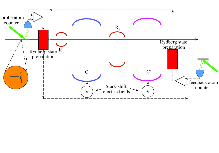
FIG. 1.: Schematic diagram of the autofeedback scheme proposed in this paper. $R_{1}$ and $R_{2}$ are the two cavities in which classical microwave pulses can be applied, $C$ is the microwave cavity of interest and $C^{\prime}$ is the cavity automatically performing the needed correction. Electric fields can be applied at the superconducting mirrors of $C$ and $C^{\prime}$ to Stark shift the Rydberg levels in order to tune the interaction times in $C^{\prime}$ and realize adiabatic transfer in $C$.

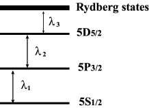
FIG. 2.: Schematic diagram of the relevant ⁸⁵Rb energy levels involved in the atom counting and in the preparation of the circular Rydberg states. The transition between the 5S_1/2 ($F=2,3$) ground state and the 5P_3/2 ($F=1,2,3,4$) first excited state is driven by a laser diode at $\lambda_{1}=780$ nm and is used for the fluorescence detection. The corresponding cycling transition is between ($F=3,m_{\rm F}=3$) and ($F^{\prime}=4,m_{\rm F}^{\prime}=4$). The transition between the first and the 5D_5/2 second excited state is driven by a laser diode at $\lambda_{2}=776$ nm. Finally, the transition between the second excited state and the Rydberg states is driven by a laser diode at $\lambda_{3}=1.26$ $\mu$m.

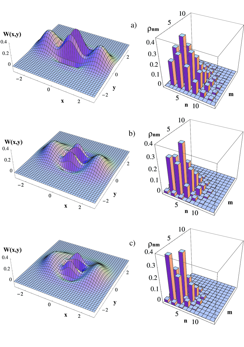
FIG. 3.: (a) Wigner function and density matrix in the photon number basis, $\rho_{n,m}=\langle n|\rho|m\rangle$, of the initial odd cat state, $|\psi\rangle=N_{-}(|\alpha\rangle-|-\alpha\rangle)$, $|\alpha|^{2}=3.3$ (b) Wigner function and density matrix $\rho_{n,m}$ of the same cat state after $13$ feedback cycles, corresponding to a mean elapsed time $\bar{t}\simeq 1/\gamma$ ($\bar{t}\simeq 6.6t_{dec}$); (c) Wigner function and density matrix $\rho_{n,m}$ of the same state after $25$ feedback cycles corresponding to a mean elapsed time $\bar{t}\simeq 2/\gamma$ ($\bar{t}\simeq 13t_{dec}$). All the parameter values are given in the text (see section V).

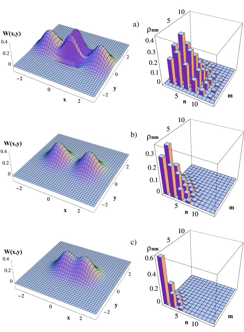
FIG. 4.: Time evolution of the same initial state of Fig. 2 in absence of feedback. (a) Wigner function and density matrix in the photon number basis, $\rho_{n,m}=\langle n|\rho|m\rangle$, of the initial odd cat state of Fig. 2; (b) Wigner function and density matrix $\rho_{n,m}$ of the same cat state after one relaxation time $t=1/\gamma$; (c) Wigner function and density matrix $\rho_{n,m}$ after two relaxation times $t=2/\gamma$. The comparison with Fig. 2 is striking: in absence of feedback the Wigner function becomes quickly positive definite, while in the presence of feedback the quantum aspects of the state remain well visible for many decoherence times.

REFERENCES

- [1] W.H. Zurek, Phys. Today 44(10), 36 (1991), and references therein.
- [2] D. Giulini, E. Joos, C. Kiefer, J. Kupsch, I.O. Stamatescu, and M.D. Zeh, Decoherence and the appearance of classical world in quantum theory, (Springer, Berlin 1996).
- [3] J. Anglin, J.P. Paz, and W.H. Zurek, Phys. Rev. A 55, 4041 (1997).
- [4] A.O. Caldeira and A.J. Leggett, Phys. Rev. A 31, 1059 (1985); D.F. Walls and G.J. Milburn, ibid 31, 2403 (1985).
- [5] C. Monroe, D.M. Meekhof, B.E. King, and D.J. Wineland, Science 272, 1131 (1996).
- [6] M. Brune, E. Hagley, J. Dreyer, X. Maitre, A. Maali, C. Wunderlich, J.M. Raimond, and S. Haroche, Phys. Rev. Lett. 77, 4887 (1996).
- [7] C.H. Bennett, in Quantum Communication, Computing and Measurement, edited by O. Hirota, A.S. Holevo and C.M. Caves (Plenum Press, New York, 1997), p. 25. See also the special issue of Physics World 11, 35 (1998) and V. Vedral and M.B. Plenio, Contemporary Physics, 39, 431 (1998).
- [8] E. Knill and R. Laflamme, Phys. Rev. A 55, 900 (1997) and references therein.
- [9] D. Bouwmeester, J.W. Pan, M. Daniell, H. Weinfurter, and A. Zeilinger, LANL e-print archive quant-ph/9810035.
- [10] E. Hagley et al., Phys. Rev. Lett. 79, 1 (1997).
- [11] Q. A. Turchette, C. S. Wood, B. E. King, C. J. Myatt, D. Leibfried, W. M. Itano, C. Monroe, and D. J. Wineland , Phys. Rev. Lett. 81, 3631 (1998).
- [12] P.T. Cochrane, G.J. Milburn, and W.J. Munro, LANL e-print archive quant-ph/9809037.
- [13] P. Tombesi and D. Vitali, Phys. Rev. A 51, 4913 (1995); P. Goetsch, P. Tombesi and D. Vitali, Phys. Rev. A 54, 4519 (1996).
- [14] D.B. Horoshko and S. Ya. Kilin, Phys. Rev. Lett. 78, 840 (1997).
- [15] D. Vitali, P. Tombesi, and G.J. Milburn, Phys. Rev. Lett. 79 2442 (1997).
- [16] D. Vitali, P. Tombesi, and G.J. Milburn, J. Mod. Opt. 44 2033 (1997).
- [17] D. Vitali, P. Tombesi, and G.J. Milburn, Phys. Rev. A 57 4930 (1998).
- [18] S. Haroche and J.M. Raimond in Cavity Quantum Electrodynamics, P. Berman ed., Academic Press, (1994), p. 123.
- [19] M. Brune, S. Haroche, J.M. Raimond, L. Davidovich, and N. Zagury, Phys. Rev. A 45, 5193 (1992).
- [20] S. Haroche, M. Brune, and J.M. Raimond, Journal de Physique II, Paris, 2, 659 (1992).
- [21] X. Maitre, E. Hagley, G. Nogues, C. Wunderlich, P. Goy, M. Brune, J.M. Raimond, and S. Haroche, Phys. Rev. Lett. 79, 769 (1997).
- [22] P. Nussenzveig, F. Bernardot, M. Brune, J. Hare, J.M. Raimond, S. Haroche, and W. Gawlik, Phys. Rev. A 48, 3991 (1993).
- [23] X. Maitre, E. Hagley, J. Dreyer, C. Wunderlich, M. Brune, J.M. Raimond, and S. Haroche, J. Mod. Opt. 44, 2023 (1997).
- [24] U. Herzog, Phys. Rev. A 53, 1245 (1996).
- [25] J.M. Raimond et al., in Laser Spectroscopy IX, M.S. Feld ed., Academic Press (1989).
- [26] A.S. Parkins, P. Marte, P. Zoller, O. Carnal, and H.J. Kimble, Phys. Rev. A 51, 1578 (1995) and references therein.
- [27] A. Messiah, Quantum Mechanics (North Holland, Amsterdam, 1962).