Quantum noise in the position measurement of a cavity mirror undergoing Brownian motion

Abstract

We perform a quantum theoretical calculation of the noise power spectrum for a phase measurement of the light output from a coherently driven optical cavity with a freely moving rear mirror. We examine how the noise resulting from the quantum back action appears among the various contributions from other noise sources. We do not assume an ideal (homodyne) phase measurement, but rather consider phase modulation detection, which we show has a different shot noise level. We also take into account the effects of thermal damping of the mirror, losses within the cavity, and classical laser noise. We relate our theoretical results to experimental parameters, so as to make direct comparisons with current experiments simple. We also show that in this situation, the standard Brownian motion master equation is inadequate for describing the thermal damping of the mirror, as it produces a spurious term in the steady-state phase fluctuation spectrum. The corrected Brownian motion master equation [L. Diosi, Europhys. Lett. 22, 1 (1993)] rectifies this inadequacy.

42.50.lc,42.50.Dv,03.65.Bz,06.30.Bp

I Introduction

Interferometers provide a very sensitive method for detecting small changes in the position of a mirror. This has been analysed extensively in the context of gravitational wave detection [2, 3, 4, 5, 6, 7] and atomic force microscopes [8, 9]. A key limit to the sensitivity of such position detectors comes from the Heisenberg uncertainty principle. The reduction in the uncertainty of the position resulting from the measurement is accompanied by an increase in the uncertainty in momentum. This uncertainty is then fed back into the position by the dynamics of the object being measured. This is called the quantum back action of the measurement, and the limit to sensitivity so imposed is referred to as the standard quantum limit. One of the pioneers in this field has been Braginsky in various studies of measurement aspects of the fluctuations of light caused by the moving mirror [10, 11].

In real devices which have been constructed so far, the quantum back action noise in the measurement record is usually small compared to that arising from classical sources of noise. However, as the sensitivity of such devices increases it is expected that we will eventually obtain displacement sensors that are quantum limited. The quantum back-action noise has not yet been seen experimentally for macroscopic devices, so seeing it is a topic of current interest. Once the standard quantum limit has been achieved, this will not be the end of the story, however. Various authors have shown that it is possible to use contractive states [12], or squeezed light [4, 13], to reduce the quantum back action and therefore increase the sensitivity of the measurement even further.

The interferometer we consider here for measuring position consists essentially of a cavity where one of mirrors is free to move. This system is also of interest from the point of view of cavity QED. Usually cavity QED experiments require optical cavities where the atomic excitations and photons in the optical modes become entangled. The dynamics follows from the interplay between these quantum variables. However, a challenging realm for cavity QED experiments involves instead an empty cavity (that is, a cavity containing no atoms or optical media) where the photons in the cavity mode interact with the motion of one of the cavity mirrors. In this scheme, the position of at least one mirror in the optical resonator is a dynamic variable. The coupling between the photons and the mirror position is simply the radiation pressure that stems from the momentum transfer of $2\hbar k$ per one reflected photon with the wavenumber $k$. It has been been shown that this system may be used to generate sub-Poissonian light in the output from the cavity [14, 15, 16]. The moving mirror alters the photon statistics by changing the optical path length in a way that is proportional to the instantaneous photon number inside the cavity. This system may also be used to create highly non-classical states of the cavity field, such as Schrödinger cats [17, 18], and might even be used to create cat states of the mirror [18]. In addition, it has been shown that such a configuration may be used to perform QND measurements of the light field [19], and to detect the decoherence of the mirror, a topic of fundamental interest in quantum measurement theory [20]. Due to recent technological developments in optomechanics, this area is now becoming experimentally accessible. Dorsel et al. have realised optical bistability with this system [21], and other experiments, particularly to probe the quantum noise, are now in progress [22, 23].

In order to create displacements that are large enough to be observed, one is tempted to use a mirror having a well-defined mechanical resonance with a very high quality factor $Q$. Thus, even when excited with weak white noise driven radiation pressure, the mirror can be displaced by a detectable amount at the mechanical resonance frequency $\nu$. For such a mirror to behave fully quantum mechanically one needs to operate at very low temperatures since the thermal energy $kT$ very easily exceeds $\hbar\nu$. For example, a $\nu/2\pi=100$ kHz resonance is already significantly excited at 5 $\mu$K. However, it is not necessary to reach the fully quantum domain to observe the quantum back action. By simultaneously combining a high optical quality factor (ie. by using a high-finesse cavity) and a specially designed low mass mirror with very high mechanical quality factor one can at typical cryogenic temperatures create conditions where the radiation pressure fluctuations (which are the source of the quantum mechanical back-action referred to earlier) exceed the effects caused by thermal noise. In this paper we discuss considerations for detecting this quantum back-action noise.

There are already a number of publications dealing with quantum noise in optical position measurements. Our main purpose here is to extend this literature in two ways which are important when considering the detection of the quantum noise. The first is the inclusion of the effects of experimental sources of noise, such as the classical laser noise and the noise from intracavity losses. The second is to perform a quantum treatment of phase-modulation detection, so that the results may be compared with those for homodyne detection. While this method of phase detection is often used in practice, it has not previously been given a quantum mechanical treatment, which we show is important because previous semiclassical treatments have underestimated the shot noise. In addition to these main objectives, we also show that the standard Brownian motion master equation is not adequate to describe the thermal damping of the mirror, but that the corrected Brownian motion master equation derived by Diosi [24] rectifies this problem.

In section II we describe the configuration of the system. In section III we perform a quantum mechanical analysis of phase modulation detection. In section IV we solve the linearised equations of motion for the cavity/mirror system, using a non-standard Brownian motion master equation which is of the Lindblad form [24]. In section V we use this solution to obtain the noise power spectral density (which we refer to simply as the spectrum) for a measurement of the phase quadrature using phase modulation detection. In the first part of this section we discuss each of the contributions and their respective forms. Next we compare the spectrum to that which results if the standard (non-Lindblad) Brownian motion master equation is used to describe the thermal damping of the mirror, and also to that which would have been obtained using homodyne detection rather than phase modulation detection. Finally we show how the error in a measurement of the position of the mirror may be obtained easily from the spectrum. We evaluate explicitly the contribution to this error from various noise sources, and plot these as a function of the laser power. Section VI concludes.

II The System

The system under consideration consists of a coherently driven optical cavity with a moving mirror which will be treated as a quantum mechanical harmonic oscillator. The light driving the cavity reflects off the moving mirror and therefore fluctuations in the position of the mirror register as fluctuations in the light output from the cavity. In the limit in which the cavity damping rate is much larger than the rate of the dynamics of the mirror (characterised by the frequency of oscillation $\nu$ and the thermal damping rate $\Gamma$) the phase fluctuations of the output light are highly correlated with the fluctuations of the position of the mirror and constitute a continuous position measurement of the mirror [8].

An experimental realisation will therefore involve a continuous phase-quadrature measurement of the light output from the cavity to determine the output spectrum of the phase-quadrature fluctuations. The nature of the detection scheme used to measure the phase quadrature is of interest to us, as we shall see that it will effect the relationship of the shot noise to the other noise sources in the measured signal. Quantum theoretical treatments usually assume the use of homodyne detection [8, 14, 15, 16]. However this is often not used in practice [25, 26]. Many current experiments use instead phase

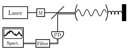
FIG. 1.: The light output from the laser is phase-modulated at frequency $\Delta$ in the modulator M, and from there drives the cavity. The front mirror of the cavity is fixed, while the back mirror is a mechanical harmonic oscillator. The diagonal line is a shorthand representation for the arrangement which isolates the laser from the cavity output, and the light that is reflected back off the front mirror. All this light falls upon a photo-detector PD, and the photo-detection signal is demodulated (to pick out the phase quadrature signal) before going to a spectrum analyser.

modulation detection [22], which was developed by Bjorklund [27, 28] in 1979. Before we treat the dynamics of the cavity field/oscillating mirror system, to determine the effect of various noise sources, we will spend some time in the next section performing a quantum mechanical treatment of phase modulation detection. We will focus on this scheme throughout our treatment, and compare the results with those for Homodyne detection. A diagram of the experimental arrangement complete enough for the theoretical analysis is given in figure 1. We note that in practice a feedback scheme is used to lock the laser to the cavity so as to stabilise the laser frequency. For an analysis of the method and an expression for the resulting classical phase noise the reader is referred to references [25] and [26]. We do not need to treat this feedback explicitly, however. Its effect may be taken into account by setting the value of the classical laser phase noise in our analysis to the level it provides.

III Phase Modulation Detection

The laser which drives the cavity is isolated from the cavity output, and the entirety of this output falls upon a photo-detector. In order that the photo-detection signal contain information regarding the phase quadrature, the laser field is modulated at a frequency $\Delta$, which is chosen to be much greater than the natural frequency of the harmonic mirror. The sidebands that result from this modulation are chosen to lie far enough off-resonance with the cavity mode that they do not enter the cavity and are simply reflected from the front mirror. From there they fall upon the photo-detector. The result of this is that the output phase quadrature signal appears in the photodetection signal as a modulation of the amplitude of a ‘carrier’ at frequency $\Delta$. This is then demodulated (by multiplying by a sine wave at the modulation frequency and time averaging) to pick out the phase quadrature signal, and from there the spectrum may be calculated.

First consider the laser output field, which is essentially classical; it is a coherent state in which the amplitude and phase are not completely stable and therefore contain some noise. This means that the field from the laser actually contains frequencies in a small range about its central frequency. The laser field may therefore be described by a set of coherent states with frequencies in this range. As a result it is possible to perform a unitary transformation on the mode operators such that the amplitude of each of the coherent states is replaced by a complex number, and the quantum state of the field is simply the vacuum [29, 30, 31]. This separates out the classical variations in the field from the quantum contribution, and allows us to write the output from the laser as

$$\beta+\delta a_{\mbox{in}}(t)+\delta x(t)+i\delta y(t)$$ (1)

In this expression $\beta$ is the average coherent amplitude of the field, which we choose to be real, and $\beta^{2}$ is the photon flux. The deviations from this average are given by $\delta x(t)$, being the classical amplitude noise, and $\delta y(t)$, being the classical phase noise. The quantum noise, which may be interpreted as arising from the vacuum quantum field, is captured by the correlation function of the field operator $\delta a_{\mbox{in}}(t)$. Here the subscript refers to the field’s relation to the cavity, and not the laser. The correlation functions of the various noise sources are

$$\langle\delta a_{\mbox{in}}(t)\delta a_{\mbox{in}}^{\dagger}(t+\tau)\rangle=\delta(\tau)$$ (2)

$$\langle\delta a_{\mbox{in}}^{\dagger}(t)\delta a_{\mbox{in}}(t+\tau)\rangle=0$$ (3)

$$\langle\delta x(t)\delta x(t+\tau)\rangle=G_{\mbox{x}}(\tau)$$ (4)

$$\langle\delta y(t)\delta y(t+\tau)\rangle=G_{\mbox{y}}(\tau),$$ (5)

where we have left the classical noise sources arbitrary. This allows them to be tailored to describe the output from any real laser source at a later time. However, we will assume that the modulation frequency, $\Delta$, is choosen large enough so that the classical noise is negligible at this frequency. This is what is done in practice. The average values of the three noise sources, $\delta a_{\mbox{in}}$, $\delta x$ and $\delta y$ are zero, as are all the cross correlations.

Before the laser field enters the cavity, it passes through a phase modulator. This is a classical device which modulates the phase of the coherent amplitude of the beam, and as such leaves the quantum noise unaffected. The phase is modulated sinusoidally, the result of which is to transform the time dependent coherent amplitude, given by $\beta+\delta x(t)+i\delta y(t)$, into [27, 32]

$$(\beta+\delta x(t)+i\delta y(t))\sum_{n=-\infty}^{n=\infty}J_{n}(M)e^{in\Delta t}$$ (6)

where $J_{n}$ is the $\mbox{n}^{\mbox{\em th}}$ Bessel function, $\Delta$ is the frequency of the modulation, and $M$ is referred to as the modulation index, being determined by the amplitude of the sinusoidal modulation. For phase modulation detection, the modulation index is typically chosen to be much less than unity so that $J_{0}\approx 1$, $J_{\pm 1}=\pm M/2\equiv\pm\varepsilon$, $\varepsilon\ll 1$, and all other terms vanish. The laser field after modulation is then

$$(\beta+\delta x(t)+i\delta y(t))(1+\varepsilon e^{-i\Delta t}-\varepsilon e^{i\Delta t})+\delta a_{\mbox{in}}(t).$$ (7)

Using now the input-output relations of Collet and Gardiner [33], the field output from the cavity is

$$a_{\mbox{out}}(t) = -(\beta+\delta x(t)+i\delta y(t))(1+\varepsilon e^{-i\Delta t}-\varepsilon e^{i\Delta t})$$ (9)

$$-\delta a_{\mbox{in}}(t)+\sqrt{\gamma}(\delta a(t)+\alpha),$$

in which $a(t)=\delta a(t)+\alpha$ is the operator describing the cavity mode, and $\gamma$ is the decay constant of the cavity due to the input coupling mirror. We are interested in the steady state behaviour, and we choose $\alpha$ to be the average steady state field strength in the cavity. In addition, in order to solve the equations of motion for the cavity we will linearise the system about the steady state, which requires that $\langle\delta a^{\dagger}(t)\delta a(t)\rangle\ll|\alpha|^{2}$. The operator describing the photo-current from the photo-detector is

  

$$I(t) = a_{\mbox{out}}(t)^{\dagger}a_{\mbox{out}}(t)$$ (10)

$$= \tilde{\alpha}^{2}+\tilde{\alpha}(\delta X_{\mbox{out}}-2\,\delta x)+2\varepsilon\beta\sin(\Delta t)\left(\delta Y_{\mbox{out}}-\frac{2\sqrt{\gamma}\alpha\,\delta y}{\beta}\right)+(2\varepsilon\beta)^{2}\sin^{2}(\Delta t)\left(1+\frac{2\,\delta x}{\beta}\right)$$ (11)

in which

$$\delta X_{\mbox{out}}(t) = \sqrt{\gamma}\,\delta X(t)-\delta X_{\mbox{in}}(t)$$ (12)

$$\delta Y_{\mbox{out}}(t) = \sqrt{\gamma}\,\delta Y(t)-\delta Y_{\mbox{in}}(t)$$ (13)

and

$$\delta X(t) = \delta a(t)+\delta a^{\dagger}(t)$$ (14)

$$\delta Y(t) = -i(\delta a(t)-\delta a^{\dagger}(t))$$ (15)

$$\delta X_{\mbox{in}}(t) = \delta a_{\mbox{in}}(t)+\delta a^{\dagger}_{\mbox{in}}(t)$$ (16)

$$\delta Y_{\mbox{in}}(t) = -i(\delta a_{\mbox{in}}(t)-\delta a^{\dagger}_{\mbox{in}}(t)).$$ (17)

We have also set $\tilde{\alpha}=(-\beta+\sqrt{\gamma}\alpha)$, and assumed this to be real. To obtain the phase quadrature signal we demodulate, which involves multiplication by a sine wave at frequency $\Delta$, and subsequent averaging over a time, $T$. This time must be long compared to $1/\Delta$, but short compared to the time scale of the phase quadrature fluctuations. The signal is therefore given by

$$R(t) = \frac{1}{T}\int_{0}^{T}\sin(\Delta\tau)I(t+\tau)\;\mbox{d}\tau,$$ (18)

We now must evaluate this to obtain $R(t)$ explicitly in terms of the phase quadrature. Writing out the integral, and dropping everything which averages to zero (that is, which is not passed by the low-pass filtering) we obtain

$$R(t) = \left(\frac{\varepsilon\beta}{T}\right)\left[\int_{0}^{T}\delta Y_{\mbox{out}}(t+\tau)d\tau\right]$$ (19)

$$- \left(\frac{2\varepsilon\sqrt{\gamma}\alpha}{T}\right)\left[\int_{0}^{T}\delta y(t+\tau)\;d\tau\right]$$ (20)

$$+ q_{1}(t)+q_{2}(t),$$ (21)

where

  

$$q_{1}(t) = -\left(\frac{\beta-\sqrt{\gamma}\alpha}{T}\right)\mbox{Re}\left[\int_{0}^{T}ie^{-i\Delta(t+\tau)}\,\delta X_{\mbox{in}}(t+\tau)\;d\tau\right],$$ (22)

$$q_{2}(t) = \left(\frac{\varepsilon\beta}{T}\right)\mbox{Re}\left[\int_{0}^{T}e^{-i2\Delta(t+\tau)}\,\delta Y_{\mbox{in}}(t+\tau)\;d\tau\right].$$ (23)

In deriving this expression we have assumed that the classical laser noise is Note that we choose $T$ to be much smaller than the time-scale upon which $\delta Y$ and $\delta y$ change, so that the integration is essentially equivalent to multiplication by $T$, an effect which is canceled by the division by $T$. However, we should also note that $\delta Y_{\mbox{out}}$ contains $\delta Y_{\mbox{in}}$, so that in replacing the first term in $R(t)$ by $\varepsilon\beta\;\delta Y_{\mbox{out}}(t)$ we must remember that this only contains the frequency components of $\delta Y_{\mbox{in}}$ in a bandwidth of $1/T$ around zero frequency. The result of this is that $\delta Y_{\mbox{out}}(t)$ is uncorrelated with $q_{1}$ and $q_{2}$, being the quantum noise in the bandwidth $1/T$ around the frequencies $\Delta$ and $2\Delta$ respectively. We need to know the correlation functions of these noise sources, and whether or not they are correlated with any of the other terms in $R(t)$. It is clear that $q_{1}$ and $q_{2}$ are not correlated over separation times greater than $2T$. Using Eq.(23) to evaluate the correlation function of $q_{2}$, for example, we have

$$\langle q_{2}(t)q_{2}(t+\tau)\rangle=\left\{\begin{array}[]{cl}\frac{(\varepsilon\beta)^{2}}{2}\left(\frac{T-|\tau|}{T^{2}}\right)&\mbox{for}\;|\tau|\leq T\\ 0&\mbox{otherwise.}\end{array}\right.$$ (24)

On the time-scale of the fluctuations of $\delta Y$ we can approximate this as a delta function, so that $q_{1}$ and $q_{2}$ (and also $\delta Y_{\mbox{in}}$) are still effectively white noise sources. We may therefore write

$$R(t) = \varepsilon\beta\;\delta Y_{\mbox{out}}(t)+q_{1}(t)+q_{2}(t)-2\varepsilon\sqrt{\gamma}\alpha\delta y(t),$$ (25)

and the correlation functions of $q_{1}$ and $q_{2}$ are

$$\langle q_{1}(t)q_{1}(t+\tau)\rangle=(1/2)(\beta-\sqrt{\gamma}\alpha)^{2}\;\delta(\tau),$$ (26)

$$\langle q_{2}(t)q_{2}(t+\tau)\rangle=(1/2)(\varepsilon\beta)^{2}\;\delta(\tau).$$ (27)

The signal therefore contains the phase quadrature of the output field, $\delta Y_{\mbox{out}}(t)$, plus three noise terms. While the last term, being the input classical phase noise, is correlated with $\delta Y_{\mbox{out}}(t)$, $q_{1}$ and $q_{2}$ are not. Taking the Fourier transform of the signal,

$$R(\omega)=\frac{1}{\sqrt{2\pi}}\int_{-\infty}^{\infty}\!\!\!\!\!\!R(t)e^{-i\omega t}\;dt,$$ (28)

we may write

$$R(\omega)=\varepsilon\beta\;\delta Y_{\mbox{out}}(\omega)+\sum_{i=1}^{2}q_{j}(\omega)-2\varepsilon\sqrt{\gamma}\alpha\,\delta y(\omega).$$ (29)

This is the Fourier transform of the signal in the case of phase modulation detection. If we were to use ideal homodyne detection this would be instead [37]

$$R_{\mbox{h}}(\omega)=\kappa\tilde{\beta}(\delta Y_{\mbox{out}}(\omega)-2\,\delta y(\omega)),$$ (30)

where $\tilde{\beta}$ is the amplitude of the local oscillator and $\kappa$ is the reflectivity of the beam splitter used in the homodyne scheme. Thus, in the case of phase modulation detection, there are two white noise sources which do not appear in homodyne detection. They stem from the fact that the phase quadrature detection method is demodulating to obtain a signal at a carrier frequency. Because the quantum noise is broad band (in particular, it is broad compared to the carrier frequency) the demodulation picks up the quantum noise at $\Delta$ and $2\Delta$. There is also a term from the classical phase noise in the sidebands. We note that the contribution from the quantum noise at $2\Delta$ has been omitted from previous semiclassical treatments, with the result that the shot noise has been underestimated by $(1/2)(\varepsilon\beta)^{2}$ [38]. For unbalanced homodyne detection there will also be an extra contribution from the noise on the local oscillator, which may be suppressed (in the limit of an intense local oscillator) with the use of balanced homodyne detection [39].

Returning to Eq.(29) for the demodulated signal, the next step is to solve the equations of motion for the system operators to obtain $\delta Y(\omega)$ in terms of the input noise sources. We can then readily calculate $\langle R(\omega)R(\omega^{\prime})\rangle$, which appears in the form

$$\langle R(\omega)R(\omega^{\prime})\rangle=S(\omega)\delta(\omega+\omega^{\prime}).$$ (31)

The delta function in $\omega$ and $\omega^{\prime}$ is a result of the stationarity of $R(t)$, and $S(\omega)$ is the power spectral density, which we will refer to from now on simply as the spectrum. This is useful because, when divided by $2\pi$, it gives the average of the square of the signal per unit frequency (The square of the signal is universally referred to as the power, hence the name power spectral density). Since the noise has zero mean, the square average is the variance, and thus the spectrum provides us with information regarding the error in the signal due to the noise. The spectrum is also a Fourier transform of the autocorrelation function [34]. The specific relation, using the definitions we have introduced above, is

$$S(\omega)=\int_{-\infty}^{\infty}\!\!\!\!\langle R(0)R(\tau)\rangle e^{-i\omega\tau}d\tau,$$ (32)

and as the autocorrelation function has units of $\mbox{s}^{-2}$, the spectrum has units of $\mbox{s}^{-1}$. To determine the spectrum experimentally the phase of the signal is measured for a time long compared to the width of the auto-correlation function, and the Fourier transform is taken of the result. Taking the square modulus of this Fourier transform, and dividing by the duration of the measurement obtains a good approximation to the theoretical spectrum. We proceed now to calculate this spectrum.

IV The Dynamics of the System

Excluding coupling to reservoirs, the Hamiltonian for the combined system of the cavity mode and the mirror is [40]

$$H = \hbar\omega_{0}a^{\dagger}a+\frac{p^{2}}{2m}+\frac{1}{2}m\nu^{2}q^{2}-\hbar ga^{\dagger}aq$$ (34)

$$+\hbar\left\{i\left[E+\sqrt{\gamma}\,\delta x(t)+i\sqrt{\gamma}\,\delta y(t)\right]a^{\dagger}+\mbox{H.c.}\right\}.$$

In this equation $\omega_{0}$ is the frequency of the cavity mode, $q$ and $p$ are the position and momentum operators for the mirror respectively, $m$ and $\nu$ are the mass and angular frequency of the mirror, $g=\omega_{0}/L$ is the coupling constant between the cavity mode and the mirror (where $L$ is the cavity length), and $a$ is the annihilation operator for the mode. The classical driving of the cavity by the coherent input field is given by $E$ which has dimensions of $\mbox{s}^{-1}$, and is related to the input laser power $P$ by $E=\sqrt{P\gamma/(\hbar\omega_{0})}=\sqrt{\gamma}\beta$. The classical laser noise appears as noise on this driving term.

The moving mirror is a macroscopic object at temperature $T$, and as such is subject to thermal noise. While it is still common to use the standard Brownian motion master equation (SBMME) [34, 41] to model such noise, as it works well in many situations, it turns out that it is not adequate for our purposes. This is because it generates a clearly non-sensical term in the spectrum. As far as we know this is the first time that it has been demonstrated to fail in the steady state. Discussions regarding the SBMME, and non-Lindblad master equations may found in references [35, 36]. We will return to this point once we have calculated the spectrum. We use instead the corrected Brownian motion master equation (CBMME) derived by Diosi [24], to describe the thermal damping of the mirror, as this corrects the problems of the SBMME. In particular, we use the CBMME in which the cut-off frequency of the thermal reservoir is assumed to be much smaller than $k_{\mbox{B}}T/\hbar$. For current experiments $k_{\mbox{B}}T/\hbar$ is greater than 10 GHz, so this assumption appears reasonable, and leads to the simplest Lindblad-form Brownian motion master equation. Using this CBMME, and the standard master equation for the cavity losses (both internal and external), the quantum Langevin equations of motion for the system are given by

$$\dot{a} = -\frac{i}{\hbar}[a,H]-\left(\frac{\gamma+\mu}{2}\right)a+\sqrt{\gamma}\,\delta a_{\mbox{in}}(t)+\sqrt{\mu}b_{\mbox{in}}(t)$$ (35)

$$\dot{q} = -\frac{i}{\hbar}[q,H]+\hbar(\Gamma/6mkT)^{\frac{1}{2}}\eta(t)$$ (36)

$$\dot{p} = -\frac{i}{\hbar}[p,H]-\Gamma p+(2m\Gamma kT)^{\frac{1}{2}}\xi(t),$$ (37)

in which the correlation functions for the Brownian noise sources are

$$\langle\xi(t)\xi(t^{\prime})\rangle = \delta(t-t^{\prime}),$$ (38)

$$\langle\eta(t)\eta(t^{\prime})\rangle = \delta(t-t^{\prime}),$$ (39)

$$\langle\xi(t)\eta(t^{\prime})\rangle = -i(\sqrt{3}/2)\delta(t-t^{\prime}),$$ (40)

$$\langle\eta(t)\xi(t^{\prime})\rangle = i(\sqrt{3}/2)\delta(t-t^{\prime}).$$ (41)

In these equations $\gamma$ is the decay constant describing transmission through the input coupling mirror. All ‘internal’ cavity losses including absorption, scattering and loss through the movable mirror are included separately via the decay constant $\mu$, and the corresponding vacuum fluctuations via the operator $b_{\mbox{in}}(t)$. The effect of mechanical damping and thermal fluctuations of the mirror are given by the noise sources $\xi(t)$ and $\eta(t)$ and the mechanical damping constant $\Gamma$.

We note here that if we were to use the standard Brownian motion master equation [41, 34], Eqs.(36) and (37) would instead be given by

$$\dot{q} = -\frac{i}{\hbar}[q,H]$$ (42)

$$\dot{p} = -\frac{i}{\hbar}[p,H]-\Gamma p+(2m\Gamma kT)^{\frac{1}{2}}\zeta(t).$$ (43)

where $\langle\zeta(t)\zeta(t^{\prime})\rangle=\delta(t-t^{\prime})$. These Langevin equations do not preserve the commutation relations of the quantum mechanical operators, and as a result it is clear that the description cannot be entirely correct.

Calculating the commutators in Eqs.(35) to (37), we obtain

  

$$\dot{a} = E-\left(\frac{\gamma+\mu}{2}\right)a+igaq+\sqrt{\gamma}\,\delta a_{\mbox{in}}(t)+\sqrt{\mu}b_{\mbox{in}}(t)+\sqrt{\gamma}\,\delta x(t)+i\sqrt{\gamma}\,\delta y(t)$$ (44)

$$\dot{q} = \frac{p}{m}+\hbar(\Gamma/6mkT)^{\frac{1}{2}}\eta(t)$$ (45)

$$\dot{p} = -m\nu^{2}q+\hbar ga^{\dagger}a-\Gamma p+(2m\Gamma kT)^{\frac{1}{2}}\xi(t).$$ (46)

Introducing a cavity detuning $\delta\omega$ (that is, setting the cavity resonance frequency in the absence of any cavity field to $\omega_{\mbox{c}}=\omega_{0}+\delta\omega$), and solving these equations for the steady state average values we obtain

$$\langle a\rangle_{\mbox{ss}} = \frac{2E}{\gamma+\mu}\equiv\alpha$$ (47)

$$\langle q\rangle_{\mbox{ss}} = \frac{\hbar g}{m\nu^{2}}|\alpha|^{2}$$ (48)

$$\langle p\rangle_{\mbox{ss}} = 0$$ (49)

where we have set the detuning to $\delta\omega=g\langle x\rangle_{\mbox{ss}}$ to bring the cavity on resonance with the driving field in the steady state. Linearising the quantum Langevin equations about the steady state values, and writing the result in terms of the field quadratures, we obtain the following linear equations

  

$$\left(\begin{array}[]{c}\delta\dot{X}\\ \delta\dot{Y}\\ \delta\dot{Q}\\ \delta\dot{P}\end{array}\right)=\left(\begin{array}[]{cccc}-\frac{\gamma+\mu}{2}&0&0&0\\ 0&-\frac{\gamma+\mu}{2}&\chi\alpha&0\\ 0&0&0&\nu\\ \chi\alpha&0&-\nu&-\Gamma\end{array}\right)\left(\begin{array}[]{c}\delta X\\ \delta Y\\ \delta Q\\ \delta P\end{array}\right)+\left(\begin{array}[]{c}\sqrt{\gamma}\,\delta X_{\mbox{in}}(t)+\sqrt{\mu}\,\delta X_{\mbox{b,in}}(t)+2\sqrt{\gamma}\,\delta x(t)\\ \sqrt{\gamma}\,\delta Y_{\mbox{in}}(t)+\sqrt{\mu}\,\delta Y_{\mbox{b,in}}(t)+2\sqrt{\gamma}\,\delta y(t)\\ (\Gamma\hbar\nu/3kT)^{\frac{1}{2}}\eta(t)\\ (4\Gamma kT/(\hbar\nu))^{\frac{1}{2}}\xi(t)\end{array}\right).$$ (50)

In this set of equations we have scaled the position and momentum variables using

$$\delta Q = \sqrt{\frac{2m\nu}{\hbar}}(q-\langle q\rangle_{\mbox{ss}})$$ (51)

$$\delta P = \sqrt{\frac{2}{m\hbar\nu}}(p-\langle p\rangle_{\mbox{ss}}).$$ (52)

and we have defined $\chi\equiv g(2\hbar/m\nu)^{1/2}$, which has units of s^-1. The quadratures for the input noise due to intracavity losses are given by

$$\delta X_{\mbox{b,in}} = b_{\mbox{in}}+b_{\mbox{in}}^{\dagger}$$ (53)

$$\delta Y_{\mbox{b,in}} = -i(b_{\mbox{in}}-b_{\mbox{in}}^{\dagger}).$$ (54)

Without loss of generality we have chosen the input field amplitude to be real ($\mbox{Im}[\beta]=0$), so that the input phase quadrature is given by $Y_{\mbox{in}}$. We now solve the dynamics (50) in the frequency domain in order to obtain the spectrum directly from the solution. To switch to the frequency domain we Fourier transform all operators and noise sources. In particular we have, for example

$$\delta a(\omega) \equiv \frac{1}{\sqrt{2\pi}}\int_{-\infty}^{\infty}\!\!\!\!\!\!\delta a(t)e^{i\omega t}\;dt,$$ (55)

$$\delta a^{\dagger}(\omega) \equiv \frac{1}{\sqrt{2\pi}}\int_{-\infty}^{\infty}\!\!\!\!\!\!\delta a^{\dagger}(t)e^{i\omega t}\;dt=[\delta a(-\omega)]^{\dagger}.$$ (56)

Rearranging the transformed equations, the solution is given by

$$(\delta X(\omega),\delta Y(\omega),\delta Q(\omega),\delta P(\omega))^{T}=M(\omega){\bf n}(\omega)$$ (57)

where ${\bf n}(\omega)$ is the vector of transformed noise sources. If we write the matrix elements of $M(\omega)$ as $M_{ij}(\omega)=m_{ij}(\omega)/D(\omega)$, then

$$D(\omega)=\left((\gamma+\mu)/2-i\omega\right)^{2}\left(\nu^{2}-\omega^{2}-i\Gamma\omega\right)$$ (58)

and the non-zero $m_{ij}$ are given by

$$m_{11} = \left((\gamma+\mu)/2-i\omega\right)\left(\nu^{2}-\omega^{2}-i\Gamma\omega\right)=m_{22},$$ (59)

$$m_{21} = \chi^{2}\alpha^{2}\nu$$ (60)

$$m_{23} = \chi\alpha(\Gamma-i\omega)\left((\gamma+\mu)/2-i\omega\right),$$ (61)

$$m_{24} = \chi\alpha\nu\left((\gamma+\mu)/2-i\omega\right)=m_{31},$$ (62)

$$m_{33} = (\Gamma-i\omega)\left((\gamma+\mu)/2-i\omega\right)^{2},$$ (63)

$$m_{34} = \nu\left((\gamma+\mu)/2-i\omega\right)^{2}=-m_{43},$$ (64)

$$m_{41} = -i\chi\alpha\omega\left((\gamma+\mu)/2-i\omega\right),$$ (65)

$$m_{44} = -i\omega\left((\gamma+\mu)/2-i\omega\right)^{2}.$$ (66)

We have now solved the equations of motion for the system in frequency space. The spectra of the system variables may now be calculated in terms of the input noise sources. Using the input-output relations, which give the output field in terms of the system variables and the input noise sources, the spectra of the output field, and hence of the measured signal, may be obtained. Note that quantum mechanics plays no role in the solution of the motion of the system. The linear equations of motion may as well be equations for classical variables. The only part that quantum mechanics plays in determining the spectra of the system variables is that some of the input noise sources are quantum mechanical. That is, their correlation functions are determined by quantum mechanics. In fact, if all the noise sources had purely classical correlation functions, then the SBMME Langevin equations would not lead to any problems, as they are perfectly correct as equations of motion for a classical system.

V The Power Spectral Density

To calculate the spectrum of the signal, we require the correlation functions of the input noise sources. To reiterate, these are

$$\langle\delta X_{\mbox{in}}(\omega)\delta X_{\mbox{in}}(\omega^{\prime})\rangle = \langle\delta Y_{\mbox{in}}(\omega)\delta Y_{\mbox{in}}(\omega^{\prime})\rangle=\delta(\omega+\omega^{\prime}),$$ (67)

$$\langle\delta X_{\mbox{in}}(\omega)\delta Y_{\mbox{in}}(\omega^{\prime})\rangle = -\langle\delta Y_{\mbox{in}}(\omega)\delta X_{\mbox{in}}(\omega^{\prime})\rangle=i\delta(\omega+\omega^{\prime}),$$ (68)

and similarly for $\delta X_{\mbox{b,in}}(\omega)$ and $\delta Y_{\mbox{b,in}}(\omega)$. The correlation functions for the classical laser noise, and thermal noise sources are

$$\langle\delta x(\omega)\delta x(\omega^{\prime})\rangle = \tilde{G}_{x}(\omega)\delta(\omega+\omega^{\prime}),$$ (69)

$$\langle\delta y(\omega)\delta y(\omega^{\prime})\rangle = \tilde{G}_{y}(\omega)\delta(\omega+\omega^{\prime}),$$ (70)

$$\langle\xi(t)\xi(t^{\prime})\rangle = \langle\eta(t)\eta(t^{\prime})\rangle=\delta(t-t^{\prime}),$$ (71)

$$\langle\eta(t)\xi(t^{\prime})\rangle = -\langle\xi(t)\eta(t^{\prime})\rangle=i(\sqrt{3}/2)\delta(t-t^{\prime}).$$ (72)

After some calculation we obtain the spectrum of the signal for phase modulation detection as

  

$$\frac{1}{(\varepsilon\beta)^{2}}S(\omega) = \frac{1}{2}\left[3+\left(\frac{\gamma-\mu}{\varepsilon(\gamma+\mu)}\right)^{2}\right]+\gamma(\gamma+\mu+4\gamma\tilde{G}_{x}(\omega))\left[\frac{(\chi^{2}\alpha^{2}\nu)^{2}}{|D(\omega)|^{2}}\right]$$ (75)

$$+\mbox{\normalsize$4\tilde{G}_{y}(\omega)$}\left[\frac{4\gamma^{2}}{(\gamma+\mu)^{2}}\left(\frac{\omega^{2}}{\left(\frac{\gamma+\mu}{2}\right)^{2}+\omega^{2}}\right)\right]$$

$$+\gamma(\chi\alpha)^{2}\Gamma\left(4\nu^{2}T_{\mbox{s}}+\frac{1}{3}(\Gamma^{2}+\omega^{2})T_{\mbox{s}}^{-1}\right)\left[\frac{\left(\frac{\gamma+\mu}{2}\right)^{2}+\omega^{2}}{|D(\omega)|^{2}}\right],$$

where

$$|D(\omega)|^{2}=\left[(\gamma+\mu)^{2}/4+\omega^{2}\right]^{2}\left[(\nu^{2}-\omega^{2})^{2}+\Gamma^{2}\omega^{2}\right],$$ (76)

and $T_{\mbox{s}}$ is a dimensionless scaled temperature given by $T_{\mbox{s}}=(k_{\mbox{B}}/(\hbar\nu))T$. This phase-fluctuation spectrum may be thought of as arising in the following way. The mechanical harmonic oscillator, which is the moving mirror, is driven by various noise sources, both quantum mechanical and classical in origin, and the resulting position fluctuations of the mirror are seen as fluctuations in the phase of the light output from the cavity.

Let us examine the origin of the various terms in the spectrum in turn. The first two terms, which appear in the first set of square brackets, are independent of the frequency, and are the contribution from the (quantum mechanical) shot noise of the light. The first term has the factor of three (rather than a factor of two which would be the case for homodyne detection) due to the contribution from $q_{2}(t)$. The second term is the contribution from $q_{1}(t)$.

The next three terms, which multiply the second set of square brackets, are the back-action of the light on the position of the mirror, noise from internal cavity losses, and the classical amplitude noise on the laser, respectively. Note that the only distinction between the back-action and the internal losses is that former is proportional to the loss rate due to the front mirror, and the latter is proportional to the internal loss rate. It is easily seen that these noise sources should have the same effect upon the position of the mirror: the back-action is due to the random way in which photons bounce off the mirror, whereas the internal losses are due to the similarly random way in which photons are absorbed by the mirror, (or anything else in the cavity). The amplitude fluctuations of the laser also affect the mirror in the same manner, but since these fluctuations are not white noise (as is the case with the quantum noise which comes from the photon ‘collisions’), the response function of the mirror is multiplied by the spectrum of the amplitude fluctuations.

The term which appears in the third set of square brackets is due to the classical phase fluctuations of the laser. Clearly this has quite a different form from that due to the quantum noise and the classical amplitude fluctuations. In particular, it is not dependent upon the coupling constant, $g$, because it is derived more or less directly from the input phase noise. Conversely, the noise that derives from the amplitude fluctuations has its origin from the fact that the amplitude fluctuations first drive the mirror, and it is the resulting position fluctuations which cause the phase fluctuations in the output. The classical phase noise term includes a contribution from the laser phase noise reflected from the cavity (that is, the term given explicitly in Eq.(29)), and a contribution from the phase noise on the light which has passed through the cavity (being a part of $Y_{\mbox{out}}$).

The final two terms, which multiply the fourth set of square brackets, are due to the thermal fluctuations of the mirror. Note that these terms are only valid in the region in which $k_{\mbox{B}}T\gg\hbar\nu$.

Finally we note that we do not see squeezing in the spectrum of phase quadrature fluctuations. This is because squeezing is produced when the cavity detuning is chosen so that the steady state detuning is non-zero [15]. We have chosen to set the steady state detuning to zero in this treatment as we are not concerned here with reducing the quantum noise.

In what follows we examine various aspects of the spectrum which are of particular interest. Before discussing considerations for detecting the back-action noise, we compare the spectrum with that which would have been obtained using the SBMME, and for that which would result from the use of homodyne detection. We then write the spectrum at resonance as a function of the laser power, and plot this for current experimental parameters. So far we have been considering the noise power spectrum, and have made no particular reference to the limit this implies for a measurement of the position of the mirror. In section V C we show how the spectrum tells us the limit to the accuracy of position measurement in the presence of the noise sources.

A Comparison with the Standard Treatment of Brownian Motion

To obtain the spectrum we have used the corrected Brownian motion master equation [24]. This is essential because the spectrum which results from the standard Brownian motion master equation contains a term which is assymetric in $\omega$, and therefore clearly incorrect. In particular, to obtain the spectrum given by the SBMME from that given by the CBMME, the term proportional to $T_{\mbox{s}}^{-1}$ must be replaced by

$$2\omega\gamma\Gamma\chi^{2}\alpha^{2}\nu\left[\frac{\left(\left(\frac{\gamma+\mu}{2}\right)^{2}+\omega^{2}\right)}{|D(\omega)|^{2}}\right].$$ (77)

That the spectrum must be symmetric in $\omega$ follows readily from the stationarity of the output field, and the fact that the output field commutes with itself at different times. In particular, the stationarity of the output field means that the correlation function of the signal only depends on the time difference, so that

$$\langle R(t)R(t+\tau)\rangle=G(\tau).$$ (78)

As the output field commutes with itself at different times, $R$ commutes with itself at different times, and we have

$$G(-\tau)=\langle R(t)R(t-\tau)\rangle=\langle R(t-\tau)R(t)\rangle=G(\tau).$$ (79)

The correlation function is therefore symmetric in $\tau$. As the spectrum is the Fourier transform of the correlation function, it follows from the properties of the Fourier transform that the spectrum is symmetric in $\omega$.

It was shown in Ref. [36] that for realistic systems at high temperatures the SBMME has a stationary density matrix which is positive. The non-Lindblad nature of the master equation appears only to cause problems at short times. In our problem we are calculating spectra at steady-state so it might seem surprising that the non-Lindbad nature does cause problems for us. On reflection, however, this is not surprising. The spectra we calculate are for continuously measured quantities. Making such measurements continuously reprepares the system in a conditioned state which is different from the stationary state. Thus if one is observing the system then it is never really at steady state and the “initial slip” problem of Ref. [36] never goes away.

Diosi’s corrected Brownian motion master equation removes the term asymmetric in $\omega$ by adding a noise source to the position (see Eq.(37)) which is correlated with the noise source for the momentum. In doing so it produces an additional term in the spectrum proportional to $1/T$, an effect which, it should be noted, is independent of the phase detection scheme. For temperatures (and frequencies) for which this new term is much smaller than the standard term, which is proportional to $T$, this new term can be neglected. However, the question of observing this term experimentally is a very interesting one, because it would allow the CBMME to be tested. Comparing the new term with the term proportional to $T$ we find that the new term begins to dominate when

$$T<\left(\frac{\hbar}{12k_{\mbox{B}}}\right)\sqrt{\Gamma^{2}+\omega^{2}}.$$ (80)

For temperatures of the order of a few Kelvin, the additional term therefore becomes apparent in the spectrum at frequencies of a few Gigahertz. Note that for such high frequencies phase modulation may no longer be practical however, owing to the fact that $\Delta$ must be much larger than the frequency range of the signal. In that case the use of alternative phase detection schemes would be required

B Comparison with Homodyne Detection

Let us now briefly compare the spectrum derived above for phase modulation detection to that which would be obtained with homodyne detection. Firstly, if homodyne detection had been used, the overall scaling of the spectrum would be different, as it would be proportional to the strength of the local oscillator. Thus the factor of $1/(\varepsilon\beta)^{2}$ would be replaced by $1/(\tilde{\beta}\kappa)^{2}$, in which $\tilde{\beta}$ and $\kappa$ are as defined in Eq. (30). This overall factor aside, two terms in the spectrum would change. The shot noise component would be reduced to unity, and the classical phase noise contribution would become

$$4\tilde{G}_{y}(\omega)\left[\frac{\left(\frac{\gamma-\mu}{2}\right)^{2}+\omega^{2}}{\left(\frac{\gamma+\mu}{2}\right)^{2}+\omega^{2}}\right].$$ (81)

C The Error in a Measurement of Position

So far we have been considering the noise spectrum of the phase quadrature, as this is what is actually measured. In this section we show how the error in a measurement of the position of the mirror may be obtained in a simple manner from the spectrum, Eq.(75), and give an example by calculating it explicitly for some of the terms. As explained above, the reason for performing the phase measurement is that it constitutes essentially a measurement of the position of the mirror.

We can choose to measure the amplitude of position oscillations at any frequency, but for the purposes of discussion, a measurement of a constant displacement is the simplest. First we must see how the position of the mirror appears in the signal, which is the phase quadrature measurement (that is, convert from the units of the signal into units of the position fluctuations). This is easily done by calculating the contribution to the spectrum of the position fluctuations due to one of the noise sources (for the sake of definiteness we will take the thermal noise), and comparing this to the equivalent term in the spectrum of the signal. This gives us the correct scaling. Performing this calculation, we find that the spectrum of position fluctuations of the mirror due to thermal noise is given by the thermal term in the spectrum (Eq.(75)), multiplied by the factor

$$\frac{\hbar}{2m(\varepsilon\beta)^{2}\gamma\nu\chi^{2}\alpha^{2}}\left(\left(\frac{\gamma+\mu}{2}\right)^{2}+\omega^{2}\right).$$ (82)

From this we see that the scaling factor is frequency dependent. This means,that the spectrum of the position fluctuations is somewhat different from the spectrum of the resulting phase quadrature fluctuations. For the measurement of the phase to correspond to a true measurement of the position the two spectra should be the same. This is true to a good approximation when $\gamma$ is much larger than the range of $\omega$ over which the spectrum of position fluctuations is non-zero, and this is why the scheme can be said to constitute a measurement of position when $\gamma\gg\nu,\Gamma$.

In performing a measurement of a constant displacement of the mirror (achieved by some constant external force), the signal (after scaling appropriately so that it corresponds to position rather than photocurrent) is integrated over a time $\tau_{\mbox{m}}$. The best estimate of the displacement is this integrated signal divided by the measurement time. The error, $\Delta x$, in the case that the measurement time is much greater than the correlation time of the noise, is given by

$$\Delta x^{2}(0)=\int_{-\infty}^{\infty}\!\!\!\!\langle R_{x}(0)R_{x}(\tau)\rangle d\tau/\tau_{\mbox{m}}=S_{x}(0)/\tau_{\mbox{m}}.$$ (83)

In this equation $R_{x}$ and $S_{x}$ are the appropriately scaled signal and spectrum. To calculate the error in the measurement of a constant displacement, all we have to do, therefore, is to scale the spectrum using the expression Eq.(82), evaluate this at zero frequency, and divide by the measurement time. In general, the spectrum evaluated at a given frequency, once divided by the measurement time, gives the error in a measurement of the amplitude of oscillations at that frequency. We calculate now the contribution to the error in a measurement at zero frequency and at the mirror resonance frequency, from the shot noise, thermal, and quantum back-action noise. In the following we write the expressions in terms of the parameters usually used by experimentalists: the laser power, $P$, cavity finesse ${\cal F}$, and the quality factor for the mirror oscillator, $Q=\nu/\Gamma$. We chose the cavity to be impedance matched, since this is usually the case in practice. This means that the decay rate due to the input coupler, $\gamma$, is chosen equal to the internal cavity decay rate, $\mu$. The total decay rate of the cavity is therefore $2\gamma$, so that the finesse is given by ${\cal F}=\pi c/(2L\gamma)$. We also assume that $\gamma\gg\nu$, which is certainly true in current experiments. Performing the calculation we find that the contribution due to the shot noise is the same at all frequencies, and is given by

$$\Delta x^{2}_{\mbox{SN}}=\frac{3\pi^{2}}{32}\left(\frac{\hbar c^{2}}{\omega_{0}}\right)\frac{1}{{\cal F}^{2}P\tau_{\mbox{m}}}.$$ (84)

The contribution from the quantum back action for a measurement of a constant displacement is

$$\Delta x^{2}_{\mbox{BA}}(0)=\frac{4}{\pi^{2}}\left(\frac{\hbar\omega_{0}}{c^{2}}\right)\left(\frac{1}{m^{2}\nu^{4}}\right)\frac{{\cal F}^{2}P}{\tau_{\mbox{m}}},$$ (85)

and for a measurement at the resonance frequency $\nu$ it is $\Delta x^{2}_{\mbox{BA}}(\nu)=Q^{2}\Delta x^{2}_{\mbox{BA}}(0)$. Note that since $\mu=\gamma$, the contribution from the internal cavity losses is also given by this expression. In a sense, the internal cavity loss noise can also be regarded as a back-action term, although the back action is from a measurement process due to the interaction with an environment that is not being observed. The total error which can be said to arise from the random ‘photon impacts’ on the mirror (in the absence of classical laser noise) is the sum of the back-action and internal loss noise, and is therefore given by

$$\Delta x^{2}_{\mbox{PN}}(0)=\frac{8}{\pi^{2}}\left(\frac{\hbar\omega_{0}}{c^{2}}\right)\left(\frac{1}{m^{2}\nu^{4}}\right)\frac{{\cal F}^{2}P}{\tau_{\mbox{m}}}.$$ (86)

The contribution from the thermal noise is

$$\Delta x^{2}_{\mbox{Th}}(0)=\left(\frac{2k_{\mbox{B}}T}{m\nu^{3}Q\tau_{\mbox{m}}}\right)+\left(\frac{\hbar^{2}}{6m\nu k_{\mbox{B}}TQ^{3}\tau_{\mbox{m}}}\right),$$ (87)

for a constant displacement, and is

$$\Delta x^{2}_{\mbox{Th}}(\nu)=\left(\frac{2k_{\mbox{B}}QT}{m\nu^{3}\tau_{\mbox{m}}}\right)+\left(\frac{\hbar^{2}Q}{6m\nu k_{\mbox{B}}T\tau_{\mbox{m}}}\right),$$ (88)

for an oscillation at the mirror frequency. In obtaining the second term in this last expression we have also used

FIG. 2.: The error in a measurement of the position of the mirror, for a measurement time of $\tau_{m}=300$s. The dashed curve corresponds to a measurement of a constant displacement, and the dot-dash curve to a measurement at the mirror resonance frequency. The combined contribution of the quantum back-action and internal cavity loss noise to both curves is the sloping section to the right. The quantum back-action noise may be observed at reasonable laser power levels. For parameters see text.

$\!\!\!\!\!\nu\gg\Gamma$. The contribution from the other noise sources may also be readily evaluated from the terms in the spectrum Eq.(75).

Let us examine the total error in a position measurement resulting from these four contributions (shot-noise, back-action, internal losses, and thermal noise) for state-of-the-art experimental parameters. Reasonable values for such parameters are as follows [22]. The laser frequency is $\omega_{0}=2\pi\times 2.82\times 10^{14}\;\mbox{rad s}^{-1}$ (assuming a Nd:YAG laser with a wavelength of 1064 nm), the cavity length is $L=1\;\mbox{cm}$, the mass of the oscillating mirror is $m=10^{-5}\;\mbox{kg}$, and the resonant frequency of the mirror is $\nu=2\pi\times 2\times 10^{4}\;\mbox{rad s}^{-1}$. The quality factor of the mirror is four million, which gives $\Gamma\approx 3\times 10^{-2}\;\mbox{s}^{-1}$. With these parameters for the cavity we have $\chi=2.29\times 10^{-4}\;\mbox{s}^{-1}$. The cavity damping rate through the front mirror is $\gamma=4.7\times 10^{5}\;\mbox{s}^{-1}$, and we assume impedance matching so that $\mu=\gamma$. The cavity may be cooled to a temperature of $T=4.2\;\mbox{K}$, so that $T_{\mbox{s}}=k_{\mbox{B}}T/(\hbar\nu)=4.37\times 10^{6}$, which is certainly in the high temperature regime ($T_{\mbox{s}}\gg 1$). The Diosi term (of order $T_{\mbox{s}}^{-2}$ at resonance) is thus totaly negligible.

In figure 2 we plot the position measurement error as a function of the laser power, both for the measurement of a constant displacement, and for a displacement at the mirror resonance frequency. The expressions for the measurement error derived above are valid in the limit where the measurement time is much greater than the correlation time of the noise. As the cavity-mirror system is driven by white noise, this correlation time is given approximately by the longest decay time of the system. In our case this is the decay time of the moving mirror, given by $1/\Gamma\approx 30\;\mbox{s}$. In view of this we have chosen a measurement time of 300 seconds (5 minutes) for the plot in figure 2.

The uncertainty due to the shot noise falls off with laser power, while that due to thermal noise is independent of laser power, and that due to the quantum back-action increases with laser power. These results are already well known. The thermal and back-action contributions are much greater at the resonance frequency of the mirror, due to the high mechanical $Q$ factor. The optimal regime for detecting the quantum back-action noise is at resonance, as the absolute magnitude of this noise is largest in this case. Reasonable experimental values for laser power lie between the solid lines, where the increase in noise due to the back-action is visible. However, our analysis of the spectrum shows us that the full situation is more complicated. We have shown that the noise due to internal cavity losses and the classical laser amplitude noise have the same dependence on frequency as the quantum back-action. In order to reach the back-action dominated regime, the laser amplitude noise must be at the shot noise level, and the frequency noise must be extremely low.

VI Conclusion

We have examined the optomechanical system consisting of a Fabry-Perot cavity containing a moving mirror to see how the quantum mechanical back-action appears among the various sources of classical noise. We have shown a number of things regarding this question. First of all, the relationship of the shot noise to the noise resulting from the oscillating mirror, and hence the limit on a position measurement due to the shot noise, is dependent on the phase measurement scheme. In particular, the result for phase modulation detection, which is commonly used in experiments of this kind, is not the same as that for homodyne detection. We have found that while the signature of the classical phase noise is quite different for that of the quantum-back action, the noise due to intracavity losses and classical amplitude noise has a very similar signature to the back-action. As far as the parameters of the cavity and oscillating mirror are concerned, realisable experiments are beginning to fall in the region where the quantum back-action may be observed.

In our treatment of the system we have shown that the standard quantum Brownian motion master equation produces a clearly spurious term in the steady state noise spectrum for the phase quadrature measurement. We have shown that the corrected Brownian motion master equation, derived by Diosi, corrects this error. However, it also produces a new term in the spectrum which is small for present experimental systems. Testing for the existence of this term poses an experimental challenge that might be met using miniature, high frequency oscillators and ultra-low temperatures.

REFERENCES

- [1]
- [2] W. A. Edelstein, J. Hough, J. R. Pugh and W. Martin, J. Phys. E 11 710 (1978).
- [3] C. M. Caves, Phys. Rev. Lett. 45, 75 (1980); R. Loudon, Phys. Rev. Lett. 47, 815 (1981); C. M. Caves, Phys. Rev. D 23 1693 (1981); M. Ley and R. Loudon, J. Mod. Optics 34, 227 (1987); P. Samphire, R. Loudon and M. Babiker, Phys. Rev. A 51, 2726 (1995).
- [4] A. F. Pace, M. J. Collett and D. F. Walls, Phys. Rev. A 47, 3173 (1993).
- [5] P. R. Saulson, Phys. Rev. D 42, 2437 (1990); K. A. Strain, K. Danzmann, J. Mizuno, P. G. Nelson, A. Rüdiger, R. Schilling and W. Winkler, Phys. Lett. A 194, 124 (1994); A. Gillespie and F. Raab, Phys. Rev. D 52, 577 (1994).
- [6] S. P. Vyatchanin and A. B. Matsko, Zh. Eksp. Teor. Fiz. 109, 1873 (1996) [JETP 82, 1007 (1996)]; S. P. Vyatchanin and A. B. Matsko, Zh. Eksp. Teor. Fiz. 110, 1253. (1996) [JETP 83 690 (1996)].
- [7] Yi Pang and J. P. Richard, Appl. Optics 34, 4982 (1995);
- [8] G. J. Milburn, K. Jacobs and D. F. Walls, Phys. Rev. A 50, 5256 (1994).
- [9] C. Schoenenberger and S. F Alvarado, Rev. Sci. Instrum. 60, 3131 (1989); L. P. Ghislain and W. W. Webb, Opt. Lett. 18, 1678 (1993); T. D. Stowe, K. Yasumura, T. W. Kenny, D. Botkin, K. Wago, and D. Rugar, Appl. Phys. Lett. 71, 288 (1997).
- [10] V. B. Braginsky and Yu. I. Vorontsov, Usp. Fiz. Nauk 114, 41 (1974)[Sov. Phys. Usp. 17, 644(1975).
- [11] V. B. Braginsky and Yu. I. Vorontsov, Usp. Fiz. Nauk 156, 93 (1988)[Sov. Phys. Usp. 31, 836(1988).
- [12] H. P. Yuen, Phys. Rev. Lett. 51, 719 (1983); W.-T. Ni, Phys. Rev. A 33, 2225 (1986); M. Ozawa, Phys. Rev. Lett. 60, 385 (1988).
- [13] W. G. Unruh, in Quantum Optics, Experimental Gravitation and Measurement Theory, edited by P. Meystre and M. O. Scully, (Plenum, New York, 1983), p. 647; R. S. Bondurant and J. H. Shapiro, Phys. Rev. D 30, 2548 (1984); M. T. Jaekel and S. Reynaud, Europhys. Lett. 13, 301 (1990); A. Luis and L. L. Sanchez-Soto, Phys. Rev. A 45, 8228 (1992).
- [14] A. Heidmann and S. Reynaud, Phys. Rev. A 50, 4237 (1994).
- [15] C. Fabre, M. Pinard, S. Bourzeix, A. Heidmann, E. Giacobino ans S. Reynaud, Phys. Rev. A 49, 1337 (1994).
- [16] M. Pinard, C. Fabre and A. Heidmann, Phys. Rev. A 51, 2443 (1995).
- [17] S. Mancini, V. I. Manko and P. Tombesi, Phys. Rev. A 55, 3042 (1997).
- [18] S. Bose, K. Jacobs and P. L. Knight, Phys. Rev. A 56, 4175 (1997).
- [19] K. Jacobs, P. Tombesi, M. J. Collett and D. F. Walls, Phys. Rev. A 49, 1961 (1994); M. Pinard, C. Fabre and A. Heidmann, Phys. Rev. A 51, 2443 (1995); A. Heidmann, Y. Hadjar and M. Pinard, Appl. Phys. B 64, 173 (1997).
- [20] S. Bose, K. Jacobs and P. L. Knight, lanl eprint: quant-ph/9712017.
- [21] A. Dorsel, J. D. McCullen, P. Meystre, E. Vignes and H. Walther, Phys. Rev. Lett. 51, 1550 (1983).
- [22] I. Tittonen, G. Breitenbach, T. Kalkbrenner, T. Müller, R. Conradt, S. Schiller, E. Steinsland, N. Blanc and N. F. de Rooij, to appear in Phys. Rev. A.
- [23] Y. Hadjar, P.F. Cohadon, C.G. Aminoff, M. Pinard, A. Heidmann, quant-ph/9901056.
- [24] L. Diosi, Europhys. Lett. 22, 1 (1993); L. Diosi, Physica A 199, 517 (1993).
- [25] D. Hils and J. L. Hall, Rev. Sci. Instrum 58, 1406 (1987).
- [26] K. Nakagawa, A. S. Shelkovnikov, T. Katsuda and M. Ohtsu, Optics Commun. 109, 446 (1994).
- [27] G. C. Bjorklund, Optics Lett. 5, 15 (1980).
- [28] G. C. Bjorklund, M. D. Levenson, W. Lenth and C. Ortiz, Appl. Phys. B 32, 145 (1983); R. W. P. Drever, J. L. Hall, F. V. Kawalski, J. Hough, G. M. Ford, A. J. Munley and H. Ward, Appl. Phys. B 31, 97 (1983).
- [29] C. W. Gardiner, Quantum Noise, (Springer, Berlin, 1991).
- [30] B. R. Mollow, Phys. Rev. A 12, 1919 (1975); C. Cohen-Tannoudji, J. Dupont-Roc, G. Grynberg, ‘Photons and Atoms’, (John Whiley & Sons, New York, 1992).
- [31] H. M. Wiseman, PhD Thesis (University of Queensland, St. Lucia ,1994).
- [32] A. Yariv, Optical Electronics (CBS College Publishing, New York, 1985).
- [33] M. J. Collett and C. W. Gardiner, Phys. Rev. A 30, 1386 (1984); C. W. Gardiner and M. J. Collett, Phys. Rev. A 31, 3761 (1985).
- [34] C. W. Gardiner, Handbook of Stochastic Methods, (Springer, Berlin, 1985).
- [35] W. J. Munro and C. W. Gardiner, Phys. Rev. A 53, 2633 (1996),
- [36] S. Gnutzmann and F. Haake, Z. Phys. B 101, 263 (1996).
- [37] H. M. Wiseman and G. J. Milburn, Phys. Rev. A 47, 642 (1993).
- [38] N. M. Sampas, PhD Thesis (University of Colorado, Bolder, 1990); N.C. Wong and J.L. Hall J.O.S.A. B 2, 1527 (1985).
- [39] H. P. Yuen and V. W. S. Chan, Opt. Lett. 8, 177 (1983).
- [40] K. Jacobs, P. Tombesi, M. J. Collett and D. F. Walls, Phys. Rev. A 49, 1961 (1994).
- [41] A. O. Caldeira and A. J. Leggett, Physica A 121, 587 (1983); A. O. Caldeira and A. J. Leggett, Phys. Rev. A 31, 1059 (1985); W. G. Unruh and W. H. Zurek, Phys. Rev. D 40, 1071 (1989).