On the Path Integral of the Relativistic Electron

Abstract

We revisit the path integral description of the motion of a relativistic electron. Applying a minor but well motivated conceptional change to Feynman’s chessboard model, we obtain exact solutions of the Dirac equation. The calculation is performed by means of a particular simple method different from both the combinatorial approach envisaged by Feynman and its Ising model correspondence.

I Introduction

It is well known that the continuum propagator of the Dirac equation can be found by summing over random walks. Renewed interest in this issue has arisen in connection with the investigation of stochastic processes which have been shown to be related to the Dirac equation (Gaveau et al. 1984, McKeon and Ord 1992). Likewise, the correspondence between the path integral and the Ising model has been explored (Gersch 1981, Jacobson and Schulman 1984) and solutions for a discretized version of the Dirac equation have been found (Kauffman and Noyes, 1996).

As described by Feynman and Hibbs (1965), the propagator of the $1+1$ dimensional Dirac equation

$$\mbox{i}{{\partial\Psi}/{\partial t}}=-\mbox{i}\sigma_{z}{{\partial\Psi}/{\partial x}}-m\sigma_{x}\Psi$$ (1)

(where units $c=\hbar=1$ are assumed and $\sigma_{x}$ and $\sigma_{z}$ are the respective Pauli spin matrices) can be found from a model of the one-dimensional motion of a relativistic particle. In this model the motion of the electron is restricted to movements either forward or backward occuring at the speed of light. Assuming units $c=1$, the motion of the particle corresponds to a sequence of straight path segments of slope $\pm 45^{\circ}$ in the x-t plane. The retarded propagator $K(x,t)$ of the Dirac equation may then obtained from the limiting process (see e.g. Feynman and Hibbs 1965, Jacobson and Schulman 1984)

$$K_{\delta\gamma}(x,t)=\lim_{N\rightarrow\infty}A_{\delta\gamma}(\epsilon)\sum_{R\geq 0}N_{\delta\gamma}(R)(\mbox{i}m\epsilon)^{R}\;.$$ (2)

Here, $N$ is the number of segments of constant length $\epsilon=t/N$ of the particle’s path between its start point (which is assumed to be the origin of the corresponding coordinate system) and the end point $(x,t)$ of the path. $R$ denotes the number of bends while $N_{\delta\gamma}(R)$ stands for the total number of paths consisting of $N$ segments with $R$ bends. The indices $\gamma$ and $\delta$ correspond to the directions forward or backward at the path’s start and end points, respectively, and refer to the components of $K$. $A_{\delta\gamma}(\epsilon)$ accounts for a convenient normalization.

II Model and Calculations

In this short note we demonstrate that a minor conceptional change of Feynman’s chessboard model naturally and directly yields exact solutions to the Dirac equation (1). The conceptional change is suggested by the observation that a path with $R$ bends between given start and end points is determined by $R-1$ bends. For a sketch of the situation consider Figure 1. The path shown in Figure 1 exhibits five bends, three to the left and two to the right. However, the first two bends to the right and left, respectively, determine the path since the location and direction of the last bend (indicated by a circle in Figure 1) is fully determined by the first four bends. We thus consider here, in contrast to the original formulation of the model where all bends occuring on a path contribute to the total amplitude, only contributions to the total amplitude from bends which actually define the path. In the light of the general path integral formalism it makes perfect sense to consider only those bends which define a path, i.e. the minimum information characterizing a path.

In the following we demonstrate by an explicit calculation that the modified model directly leads to exact solutions of the Dirac equation (1). We will use a calculation scheme different from the combinatorial approach envisaged by Feynman and Hibbs (1965) and its Ising model correspondence (Gersch, 1981). Following Feynman’s chessboard model we consider each bend which defines a possible path to contribute an amplitude

$$\phi_{j_{r}}=\mbox{i}m\epsilon_{j_{r}}$$ (3)

where $\epsilon_{j_{r}}\doteq\epsilon$ is the length of a path segment. The total amplitude contributed by a path is the product

$$\phi=\prod_{r}(\mbox{i}m\epsilon_{j_{r}})$$ (4)

where $j_{r}$ runs over all the segments followed by a bend. While the index $r$ enumerates the path segments after which bends occur, the value of $j_{r}$ indicates the corresponding segment. A path with $R$ bends which starts with positive velocity (i.e. to the right) and ends with negative velocity (i.e. to the left) consists of exactly $(R-1)/2+1$ bends to the left and $(R-1)/2$ to the right. The $(R-1)/2$ bends to the right may occur after any arbitrary path segment to the left. $(R-1)/2$ of the $(R-1)/2+1$ bends to the left occur in the same manner after path segments to the right while the additional bend to the left occurs after the last segment. Let $P$ be the total number of path segments to the right (+) and $Q$ those to the left (-). Then, the contribution of the $R^{+}=(R-1)/2$ bends to the right to $\Psi_{-+}$ is

$$\Psi_{-+}(R^{+}) = N_{-+}(R^{+})\prod^{R^{+}}_{r=1}(\mbox{i}m\epsilon_{j_{r}})$$ (5)

$$= \sum^{P-1}_{j_{1}<\ldots<j_{R^{+}}}(\mbox{i}m\epsilon)^{R^{+}}$$ (6)

For $P\gg 1$, $\Psi_{-+}(R^{+})$ is approximated by

$$\Psi_{-+}(R^{+}) \approx {1\over{{R^{+}}!}}\sum^{P}_{j_{1}\neq\ldots\neq j_{R^{+}}}(\mbox{i}\epsilon)^{R^{+}}$$ (7)

$$\approx {(\mbox{i}m\epsilon)^{R^{+}}\over{{R^{+}}!}}\left(\sum_{j_{r}=1}^{P}1\right)^{R^{+}}$$ (8)

$$= {P^{R^{+}}(\mbox{i}m\epsilon)^{R^{+}}\over{{R^{+}}!}}$$ (9)

The contribution of the $R^{-}=[((R-1)/2+1)-1]=(R-1)/2$ bends to the left is calculated similarly. The additional bend (occuring after the last segment to the right) does not enter the calculation since a possible path is fully determined by the location by its $R-1$ bends to the right and left, respectively. Therefore we find

$$\Psi_{-+}(R^{-}) \approx {Q^{R^{-}}(\mbox{i}\epsilon)^{R^{-}}\over{{R^{-}}!}}$$ (10)

In the limit $N\rightarrow\infty$ (i.e. $P,Q\rightarrow\infty$) the exact expression for $\Psi_{-+}$ becomes

$$\Psi_{-+}=\sum_{\mbox{odd }R}(\mbox{i}m\epsilon)^{R-1}{(PQ)^{(R-1)/2}\over{[((R-1)/2)!]^{2}}}$$ (11)

where $\epsilon=t/(P+Q)$. With $v={\Delta x/{\Delta t}}=x/t={{(P-Q)}/{(P+Q)}}$ the classical velocity attributed to the particle, $PQ=((P+Q)/2\gamma)^{2}$ where $\gamma=1/\sqrt{1-v^{2}}$. Thus we have

$$\Psi_{-+}=\sum^{\infty}_{k=0}(-1)^{k}{({mt/{2\gamma}})^{2k}\over{[(k)!]^{2}}}=J_{0}(mt/\gamma)$$ (12)

where $J_{0}$ is the zeroth order Bessel function of the first kind. A similar calculation yields for $\Psi_{+-}$ the same result.

For $\Psi_{++}$, the number of bends to the right and to the left is $R/2$ for each direction where $R$ is even. However, the path is again defined by $R^{+}=R/2$ bends to the right and $R^{-}=R/2-1$ bends to the left. Thus,

$$\Psi_{++} = \sum_{\mbox{even }R}(\mbox{i}m\epsilon)^{R-1}{P^{R/2}Q^{R/2-1}\over{(R/2)!(R/2-1)!}}$$ (13)

$$= \mbox{i}\sqrt{{P/{Q}}}\sum^{\infty}_{k=0}(-1)^{k}{(mt/2\gamma)^{2k+1}\over{(k+1)!(k)!}}$$ (14)

$$= \mbox{i}\sqrt{{P/{Q}}}J_{1}(mt/\gamma)\;.$$ (15)

With $\sqrt{{P/{Q}}}=(t+x)/(t^{2}-x^{2})^{1/2}$ and $\tau=(t^{2}-x^{2})^{1/2}$ the component $\Psi_{++}$ becomes

$$\Psi_{++}=\mbox{i}(t+x)/\tau\,J_{1}(mt/\gamma)\,.$$ (16)

A similar calculation yields

$$\Psi_{--}=\mbox{i}(t-x)/\tau\,J_{1}(mt/\gamma)\,.$$ (17)

This completes the envisaged computation. As a side remark note that the presented calculation scheme is not restricted to $\epsilon_{j_{r}}\doteq\epsilon$. As will be shown elsewhere, similar results may be obtained for $\epsilon_{j_{r}}=\epsilon(j_{r})$.

III Discussion

To relate the components $\Psi_{\delta\gamma}$ to the solution of the Dirac equation (1) consider the explicit represation

$$\sigma_{x}=\left(\begin{array}[]{cc}0&1\\ 1&0\end{array}\right),\quad\sigma_{z}=\left(\begin{array}[]{cc}1&0\\ 0&-1\end{array}\right)\;.$$ (18)

As may be seen by direct calculation, in this representation $\Psi_{1}$ and $\Psi_{2}$ defined as

$$\Psi_{1}=\left(\begin{array}[]{c}\Psi_{++}\\ \Psi_{+-}\end{array}\right);\quad\Psi_{2}=\left(\begin{array}[]{c}\Psi_{+-}\\ \Psi_{--}\end{array}\right)$$ (19)

are two independent, exact solutions of the Dirac equation (1). This completes the demonstration that Feynman’s chessboard model yields exact solutions to the Dirac equation when taking into account only those bends which actually define paths. With regard to fundamental theories of spacetime and/or quantum mechanics (e.g. in the spirit of Finkelstein, 1974) this could be of importance. Somehow similar results have been obtained from the continuum limit of a discretized version of the Dirac equation (Kauffman and Noyes, 1996).

The calculation scheme and part of the results presented here can be generalized to unevenly spaced spacetime lattices. This opens up the possibility to define an analogon to the Feynman checkerboard for discrete spacetime models of different type (e.g. Kull and Treumann, 1994). Related work is in progress and will be presented elsewhere.

A.K. would like to thank Dr. O. Forster for valuable discussions. Part of the work of A.K. has been supported by the Swiss National Foundation, grant 81AN-052101.

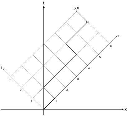
FIG. 1.: A possible path with five bends between given start and end points. The first two bends to the right and left, respectively, determine the path since the location and direction of the last bend (indicated by a circle) is fully determined by the first four bends.

REFERENCES

- [1] R. P. Feynman and A. R. Hibbs, Quantum Mechanics and Path Integrals (McGraw-Hill, New York, 1965), p. 34-36.
- [2] D. Finkelstein, Phys. Rev. D 9, 2219 (1974) and references therein.
- [3] B. Gaveau, T. Jacobson, M. Kac, and L. S. Schulman, Phys. Rev. Lett. 53, 419 (1984).
- [4] H. A. Gersch, Int. J. Theor. Phys. 20, 491 (1981).
- [5] T. Jacobson and L. S. Schulman, J. Phys. A. 17, 275 (1984).
- [6] L. H. Kauffman and H. P. Noyes, Phys. Lett. A, 218, 139 (1996).
- [7] A. Kull and R. A. Treumann, Int. J. Theor. Phys. 34, 3, 435 (1994)
- [8] D. G. C. McKeon and G N. Ord, Phys. Rev. Lett. 69, 3 (1992).