Measuring the entangled Bell and GHZ aspects using a single-qubit shuttle

Abstract

A complete, non-demolition procedure is established for measuring multi-qubit entangled states, such as the Bell-states and the GHZ-states, which is essential in certain processes of quantum communication, computation, and teleportation. No interaction between the individual parts of the entangled system, nor with any environment is required. A small probe (e.g. a single qubit) takes care of all interaction with the system, and is used repeatedly. The probe-qubit interaction is of the simplest form, and only this one type of interaction is required to perform a complete measurement. The process may be divided into elementary local operations and interactions, taking place sequentially as the probe visits each of the qubits. A shuttle mode is described, which may be repeated indefinitely. By the quantum Zeno effect, the entangled states can be maintained until released in a predictable state. This shuttle process is stable, and self-correcting, by virtue of the standard measurements performed repeatedly on the probe.

I Introduction

Quantum entanglement is one of the most remarkable manifestations of the fundamental principles. Consider two distinguishable systems, with quantum states ${|\,\psi_{i}\,\rangle}$ and ${|\,\phi_{i}\,\rangle}$, $i=1,2\cdots$. When these systems are independent, then their joint state is separable, as for instance ${|\,\psi_{1}\,\rangle}\otimes{|\,\phi_{1}\,\rangle}$, or ${|\,\psi_{2}\,\rangle}\otimes{|\,\phi_{2}\,\rangle}$. However, according to the principle of superposition, the compound system may also exist in states that are not separable, such as

$\displaystyle{|\,\Psi\,\rangle}=c_{1}{|\,\psi_{1}\,\rangle}\otimes{|\,\phi_{1}\,\rangle}+c_{2}{|\,\psi_{2}\,\rangle}\otimes{|\,\phi_{2}\,\rangle}+\cdots$

where $c_{1},c_{2},\cdots$ are complex amplitudes. This possibility has given rise to many profound discussions, in particular concerning the EPR paradox and the Bell inequalities [2, 3]. It has been confirmed—beyond any reasonable doubt—that these entangled states are uniquely a quantum phenomenon [4, 5, 6].

There have been many proposals for preparing specific entangled states, starting with suitably initialized states, such as for instance [7, 8, 9, 10, 11, 12], and this has been achieved in new ways, for Bell-states [13, 14, 15, 16] (notation, cf. Sect. II A)

$${|\,\Phi^{\pm}\,\rangle} = \textstyle{1\over{\sqrt{2}}}\bigl{(}{|\,\!\uparrow\uparrow\,\rangle}\pm{|\,\!\downarrow\downarrow\,\rangle}\bigr{)}$$

$${|\,\Psi^{\pm}\,\rangle} = \textstyle{1\over{\sqrt{2}}}\bigl{(}{|\,\!\uparrow\downarrow\,\rangle}\pm{|\,\!\downarrow\uparrow\,\rangle}\bigr{)}$$

and for GHZ-states [17, 18, 19, 20, 21]

$\displaystyle{|\,\Xi^{\pm}\,\rangle}=\textstyle{1\over{\sqrt{2}}}\bigl{(}{|\,\!\uparrow\uparrow\uparrow\,\rangle}\pm{|\,\!\downarrow\downarrow\downarrow\,\rangle}\bigr{)}$

Recent experiments have demonstrated that it is feasible to design processes that depend in an essential way on handling such entangled states. This includes quantum communication [22], quantum computation [23, 24, 25, 26, 27, 28, 29], and quantum teleportation [30, 31, 32, 33, 34]. For instance, in densely coded quantum communication the receiving party must measure the Bell-states in order to retrieve the encoded information [35]. In quantum teleportation [36] the executive step is also a measurement of the entangled Bell-states, or an EPR-state [37, 38]. This projects the entire system into the teleporting configuration, and, at the same time, acquires the data that must be transmitted by classical means.

In order to perform such a measurement one has to design a global experimental situation for the compound system. For pairs of photons, interferometric methods can provide characteristic detection patterns, which more or less completely distinguish the entangled states from each other [30, 32, 39, 40, 41, 42, 43]. Unless interaction is possible a complete Bell-state measurement is not feasible [44, 45]. In [31], where the entangled components are the polarization and momentum of a single photon, all the Bell-states can be distinguished by using polarizing beam-splitters [46]. In this situation the entangled subsystems (i.e. polarization and momentum of a single photon) are made to interact directly with each other. That is also the case in a recent NMR based teleportation experiment [34]. In these procedures, what amounts to a controlled-NOT operation disentangles the Bell-states [47, 48], and one can then measure the now separate subsystems. The entangled state is destroyed in these types of measurement.

However, states of known entanglement are becoming a resource. It will be desirable to retain the entangled system itself after the measurement, for subsequent processing—not merely the data acquired.

Also, from a more fundamental point of view, in order to establish entanglement as a standard physical observable, one really needs a non-demolition procedure. That is, a procedure which leaves any of the properly entangled states invariant, while delivering unambiguous information about it. A method of this nature has been proposed for the Bell-states and other entangled states of a similar structure in [37, 49]. In this design, the measuring device itself consists of components that must be prepared beforehand into entangled states. After these components have been placed at the relevant locations, an instantaneous non-local measurement can be performed, at least in principle.

The measurement procedure established in the present paper is different from the existing ones in several respects. It is both simple and economical of resources that appear to remain scarce, at least within a foreseeable future. The ‘apparatus’ can be as small as a single-qubit probe, which is used repeatedly according to a predesigned shuttle schedule. In principle, this allows a complete measurement of the entangled basis-states of any number of target qubits. The necessary interactions have been reduced to bare essentials, so that only the most elementary operations are involved at every stage of the procedure. In particular, no entanglement is required at the outset. For example, it is possible to imagine a single ${}^{13}\text{C}$ nuclear spin probe, paying simultaneous attention to a number of different H qubits.

Since the method relies on a traveling probe, it conforms in a straightforward way with special relativity. On the other hand, this means that it is not capable of instantaneous measurement at space-like separation. However, it seems that it could be efficient in combination with entanglement swapping, in creating distant multi-qubit entangled states [8, 12].

Sect. II describes the principles of the procedure for measuring the Bell-states of two qubits. Examples include both a spin $1/2$, and a single-mode cavity-field probe. Sect. III entends these methods to systems of arbitrary numbers of qubits, and provides an extensive analysis of the GHZ-states of three qubits. For both cases a shuttle design is provided, which permits the measurement to be continued indefinitely, with a sustained flow of measurement data. In effect, this could provide stable storage for entangled states, which can then (in principle, of course) be extracted with certainty at a predetermined time, using the acquired data.

II Measuring the Bell-aspect

A Definitions

Consider two qubits, labeled 1 and 2, and represented as distinguishable spin $1/2$ systems with Pauli spin operators $\vec{\sigma}=(\sigma_{x},\sigma_{y},\sigma_{z})$. Let $\sigma_{z}{|\!\uparrow\,\rangle}={|\!\uparrow\,\rangle}$ and $\sigma_{z}{|\!\downarrow\,\rangle}=-{|\!\downarrow\,\rangle}$, and write their joint states in the form

$${|\,\!\uparrow\downarrow\,\rangle}\equiv{|\!\uparrow\,\rangle}^{(1)}\otimes{|\!\downarrow\,\rangle}^{(2)}$$

The Bell-states form an orthonormal basis of (maximally) entangled two-qubit states

$${|\,\Psi^{\pm}\,\rangle} = \textstyle{1\over{\sqrt{2}}}\bigl{(}{|\,\!\uparrow\downarrow\,\rangle}\pm{|\,\!\downarrow\uparrow\,\rangle}\bigr{)}$$ (2)

$${|\,\Phi^{\pm}\,\rangle} = \textstyle{1\over{\sqrt{2}}}\bigl{(}{|\,\!\uparrow\uparrow\,\rangle}\pm{|\,\!\downarrow\downarrow\,\rangle}\bigr{)}$$ (3)

These states are simultaneous eigenstates of the commuting operators

$$\sigma_{xx} \equiv \sigma_{x}^{(1)}\otimes\sigma_{x}^{(2)}$$ (4)

$$\sigma_{yy} \equiv \sigma_{y}^{(1)}\otimes\sigma_{y}^{(2)}$$ (5)

$$\sigma_{zz} \equiv \sigma_{z}^{(1)}\otimes\sigma_{z}^{(2)}$$ (6)

with eigenvalues $\pm 1$. They are therefore also eigenstates of the ‘Bell-operators’ [13, 50]

$$B_{\text{CHSH}}=\sqrt{2}\bigl{(}\sigma_{xx}\pm\sigma_{yy}\bigr{)}$$

The eigenvalues $\pm 2\sqrt{2}$ signal a maximal violation of the corresponding Bell-inequalities, in the well-known way. The combination of this set of compatible observables, and their basis states, will be referred to as the ‘Bell-aspect’ [51].

The eigenvalue of $\sigma_{xx}$ determines the ‘e/o question’, i.e. whether the state is even or odd (e/o) under global spin flip. The eigenvalue of $\sigma_{zz}$ determines the ‘p/a question’, whether the spins are parallel or antiparallel (p/a). The corresponding projectors are

$$\bar{P}_{a}=\textstyle{1\over 2}\bigl{(}1+a\sigma_{xx}\bigr{)} \quad a=\pm 1$$ , (7)

$$P_{b}=\textstyle{1\over 2}\bigl{(}1+b\sigma_{zz}\bigr{)} \quad b=\pm 1$$ , (8)

Consequently, the Bell-aspect is defined by the one-dimensional projectors

$$P_{ab}=\textstyle{1\over 4}\bigl{(}1+a\sigma_{xx}\bigr{)}\bigl{(}1+b\sigma_{zz}\bigr{)}$$ (9)

A complete measurement can therefore be done in two stages. Each stage consists of a partial measurement separately deciding the p/a and e/o questions. The relevant procedures must commute, as the projectors (7) and (8) do.

Let a bilateral rotation of the two spins, by $-\pi/2$ about the global y-axis, be written as

$$U_{yy}\equiv U_{y}\otimes U_{y},\quad U_{y}=\textstyle{1\over{\sqrt{2}}}\bigl{(}{1+i\sigma_{y}}\bigr{)}$$

Then

$$\sigma_{x}=U_{y}^{\dagger}\sigma_{z}U_{y},\quad{\left(U_{y}\right)}^{2}=i\sigma_{y}$$

Using the algebra of the Kronecker product one gets

$$\sigma_{xx} = U_{yy}^{\dagger}\sigma_{zz}U_{yy}$$

$$\sigma_{yy} = -{\left({U_{yy}}\right)}^{2}=-{\left({U_{yy}^{\dagger}}\right)}^{2}$$

Therefore

$$P_{ab}=-\textstyle{1\over 4}\sigma_{yy}U_{yy}\bigl{(}1+a\sigma_{zz}\bigr{)}U_{yy}\bigl{(}1+b\sigma_{zz}\bigr{)}$$ (10)

This suggests a simplified two-stage procedure, consisting of identical operations $U_{yy}\left(1+a\sigma_{zz}\right)$. Here one first decides the p/a question, then one rotates the spins bilaterally. With such a chain of operations, the measurement is reduced to the most economical form, with respect to the resources that will be needed to carry it out in practice. In particular, only one type of unilateral rotation, $U_{y}$, is required. The essential task is to perform the partial p/a measurement, but also here only a single procedure is necessary. What is more, each partial measurement is a binary test. It therefore requires no more than a single spin $1/2$, repeatedly probing the qubits.

B Spin $1/2$ probe

Let the probe eigenstates in the xy-plane be denoted ${|\,\text{E}\,\rangle}$, ${|\,\text{W}\,\rangle}$, ${|\,\text{N}\,\rangle}$, and ${|\,\text{S}\,\rangle}$, i.e.

$$\sigma_{x}{|\,\text{E}\,\rangle}={|\,\text{E}\,\rangle} \quad\sigma_{x}{|\,\text{W}\,\rangle}=-{|\,\text{W}\,\rangle}$$ ,

$$\sigma_{y}{|\,\text{N}\,\rangle}={|\,\text{N}\,\rangle} \quad\sigma_{y}{|\,\text{S}\,\rangle}=-{|\,\text{S}\,\rangle}$$ ,

$$\sigma_{z}{|\,\text{E}\,\rangle}={|\,\text{W}\,\rangle} \quad\sigma_{z}{|\,\text{W}\,\rangle}={|\,\text{E}\,\rangle}$$ ,

The corresponding projectors are written

$$P_{\text{E}}={|\,\text{E}\,\rangle}{\langle\,\text{E}\,|} \quad P_{\text{W}}={|\,\text{W}\,\rangle}{\langle\,\text{W}\,|}$$ , (11)

$$P_{\text{N}}={|\,\text{N}\,\rangle}{\langle\,\text{N}\,|} \quad P_{\text{S}}={|\,\text{S}\,\rangle}{\langle\,\text{S}\,|}$$ , (12)

In the following, $\vec{\sigma}=(\sigma_{x},\sigma_{y},\sigma_{z})$ (with no superscript) stands for the Pauli operators of this probe. The explicit $\otimes$ separates the probe and the qubit operators.

The interaction between a single qubit and the probe is taken to be of the simplest possible form

$$U_{1}=\exp(-i\theta\sigma_{z}\otimes\sigma_{z}^{(1)}/2)$$

The parameter $\theta$ can be adjusted by controlling the length of time during which the probe interacts with qubit 1. This type of interaction can be realized in different systems, including nuclear spins, where it is standard, and by dispersive Rydberg-atom/cavity-field interaction (described in the following, cf. Sect. II H). It allows the entire measurement process to be reduced to elementary operations. This strategy is of course familiar from NMR work, for instance, which establishes its feasibility.

A similar interaction with qubit 2 gives

$$U_{2}=\exp(-i\theta\sigma_{z}\otimes\sigma_{z}^{(2)}/2)$$

It does not matter if these interactions with the qubits take place simultaneously, or one after the other. All operators commute, and

$$U_{2}U_{1}=\exp(-i\theta\sigma_{z}\otimes S_{z})$$

where

$$S_{z}={\textstyle{1\over 2}}\bigl{(}{\sigma_{z}^{(1)}+\sigma_{z}^{(2)}}\bigr{)}$$

Extend the definitions (5) to include the unit operators, such that for instance

$$\sigma_{z0}\equiv\sigma_{z}^{(1)}\otimes 1^{(2)}$$

Then one can use $\sigma_{0z}=\sigma_{z0}\sigma_{zz}$ to write

$$S_{z}={\textstyle{1\over 2}}\left({\sigma_{z0}+\sigma_{0z}}\right)=\sigma_{z0}P_{+}=\sigma_{0z}P_{+}$$ (13)

The projector is given by (8). For $j=1,2,\ldots$

$$\left({\sigma_{z}\otimes\sigma_{z0}P_{+}}\right)^{2j} = 1\otimes P_{+}$$

$$\left({\sigma_{z}\otimes\sigma_{z0}P_{+}}\right)^{2j+1} = \left({\sigma_{z}\otimes\sigma_{z0}}\right)\left({1\otimes P_{+}}\right)$$

Therefore

$$U_{2}U_{1} = 1\otimes 1+\left({\cos\theta-1}\right)\left({1\otimes P_{+}}\right)$$ (15)

$$-i\sin\theta\left({\sigma_{z}\otimes\sigma_{z0}}\right)\left({1\otimes P_{+}}\right)$$

$$= 1\otimes P_{-}$$ (17)

$$+\left({\cos\theta-i\sin\theta\;\sigma_{z}\otimes\sigma_{z0}}\right)\left({1\otimes P_{+}}\right)$$

For $\theta=\pi/2$ then

$$U_{2}U_{1}=1\otimes P_{-}-i\sigma_{z}\otimes\sigma_{z0}P_{+}$$ (18)

Here $\sigma_{z}$ rotates the probe spin, while $\sigma_{z0}$ swaps the qubit Bell-states, e.g.

$$\sigma_{z0}{|\,\Phi^{\pm}\,\rangle}={|\,\Phi^{\mp}\,\rangle}$$

Because of the $P_{+}$ projector, both of these operations take place only when the qubit spins are in the parallel subspace spanned by $\Phi^{\pm}$.

C The partial measurement (p/a)

Let the initial states of the probe and qubits be given by statistical operators (density matrices) $v$ and $w$, respectively. Suppose the probe is initialized along the positive x-direction, so that the joint state is

$$\rho=v\otimes w,\quad v=P_{\text{E}}$$

After the probe-qubit interactions one has

$$\rho^{\prime} = U_{2}U_{1}\;\rho\;U_{1}^{\dagger}U_{2}^{\dagger}$$

$$= {|\,\text{E}\,\rangle}{\langle\,\text{E}\,|}\otimes P_{-}wP_{-}$$

$$+{|\,\text{W}\,\rangle}{\langle\,\text{W}\,|}\otimes\sigma_{z0}P_{+}wP_{+}\sigma_{z0}$$

$$+i\,{|\,\text{E}\,\rangle}{\langle\,\text{W}\,|}\otimes P_{-}wP_{+}\sigma_{z0}$$

$$-i\,{|\,\text{W}\,\rangle}{\langle\,\text{E}\,|}\otimes\sigma_{z0}P_{+}wP_{-}$$

One can now read the probe by any ordinary, local measurement, coupling it to a suitable apparatus, possibly including a large environment. As far as the probe and qubit degrees of freedom are concerned, this is equivalent to the operation

$$\rho^{\prime}_{\text{meas}} = \left({P_{\text{E}}\otimes 1}\right)\rho\left({P_{\text{E}}\otimes 1}\right)$$ (20)

$$+\left({P_{\text{W}}\otimes 1}\right)\rho\left({P_{\text{W}}\otimes 1}\right)$$

That is, none of this should affect the qubit pair. Measuring the probe spin in the x-direction then gives

$$\rho^{\prime}_{\text{meas}}=P_{\text{E}}\otimes P_{-}wP_{-}+P_{\text{W}}\otimes\sigma_{z0}P_{+}wP_{+}\sigma_{z0}$$ (21)

This represents the acquisition of binary data, ‘E’ or ‘W’ corresponding to the distinct alternatives of the p/a test. The (reduced) state of the qubit-pair is not affected by these interactions between the probe and the external apparatus

$$w^{\prime} = \text{tr}_{\text{probe}}(\rho^{\prime})=\text{tr}_{\text{probe}}(\rho^{\prime}_{\text{meas}})$$

$$= P_{-}wP_{-}+\sigma_{z0}P_{+}wP_{+}\sigma_{z0}$$

The statistics of the data is that, one obtains the item E a fraction of the times given by

$$\text{tr}\bigl{(}{(P_{\text{E}}\otimes 1)\rho^{\prime}(P_{\text{E}}\otimes 1)}\bigr{)} = \text{tr}_{12}(P_{-}wP_{-})$$

$$= \text{tr}_{12}(wP_{-})\equiv p_{-}$$

This equals the estimated probability, $p_{-}$, for anti-parallel spins in the initial qubit state $w$. Likewise, one gets W with a frequency

$$\text{tr}_{12}(\sigma_{z0}P_{+}wP_{+}\sigma_{z0})=\text{tr}_{12}(wP_{+})\equiv p_{+}$$

D Probe motion

It is also of interest to monitor the probe spin in the course of time during the interaction with the qubits. The reduced probe state at a time corresponding to $\theta$ is given by (using (17))

$$v(\theta) = \text{tr}_{12}(U_{2}U_{1}\,\rho\,U_{1}^{\dagger}U_{2}^{\dagger})$$

$$= \left({p_{-}+p_{+}\cos^{2}\theta}\right)v+p_{+}\sin^{2}\theta\;\sigma_{z}v\sigma_{z}$$

$$+i\sin\theta\cos\theta\;\langle S_{z}\rangle\left({v\sigma_{z}-\sigma_{z}v}\right)$$

Here, according to (13),

$$\langle S_{z}\rangle = \text{tr}_{12}(w\sigma_{z0}P_{+})$$

$$= {\langle\,\Phi^{-}\,|}\>w\>{|\,\Phi^{+}\,\rangle}+{\langle\,\Phi^{+}\,|}\>w\>{|\,\Phi^{-}\,\rangle}$$

$$= {\langle\,\uparrow\uparrow\!\,|}\>w\>{|\,\!\uparrow\uparrow\,\rangle}-{\langle\,\downarrow\downarrow\!\,|}\>w\>{|\,\!\downarrow\downarrow\,\rangle}$$

This quantity is zero in all the Bell-states, but not in the triplet states where $S_{z}=\pm 1$. The probe spin polarization is

$$\vec{m}(\theta)=\text{tr}_{\text{probe}}\bigl{(}v(\theta)\,\vec{\sigma}\bigr{)}$$

This gives

$$m_{x}(\theta) = \bigl{(}{p_{-}+p_{+}\cos 2\theta}\bigr{)}\;m_{x}(0)-\sin 2\theta\;\langle S_{z}\rangle\;m_{y}(0)$$

$$m_{y}(\theta) = \bigl{(}{p_{-}+p_{+}\cos 2\theta}\bigr{)}\;m_{y}(0)+\sin 2\theta\;\langle S_{z}\rangle\;m_{x}(0)$$

$$m_{z}(\theta) = m_{z}(0)$$

For a large ensemble this motion may be detectable, and would then provide information about $w$ in terms of the mean values $p_{\pm}$ and $\langle S_{z}\rangle$. If no probe measurement is made, then (disregarding decoherence) everything eventually returns to the initial state $\rho$. On the other hand, in the measurement situation, where one starts at $\vec{m}=(1,0,0)$, one gets instead at $\theta=\pi/2$

$$v^{\prime}=p_{-}P_{\text{E}}+p_{+}P_{\text{W}}$$

and

$$m_{x}(\pi/2) = p_{-}-p_{+}$$

$$m_{y}(\pi/2) = m_{z}(\pi/2)=0$$

Of course, a measurement on the probe at this stage removes its coherence with the qubit pair, as it should, and the probe-qubit system therefore cannot return to the initial state. The data thus acquired determines the initial state of each individual probe-qubit system in the subsequent evolution. In the case of W this means that the probe will be in the state $P_{\text{W}}$, and, at the same time, the qubit pair state is projected into the parallel subspace. This occurs with a statistical frequency equal to the probability $p_{+}$.

E Repeated measurement

One can cancel the $\Phi^{\pm}$ permutation due to $\sigma_{z0}$ by performing a repeated measurement, using the output as new input. Then, using (21) as initial state, either

$$P_{\text{E}}\otimes P_{-}wP_{-}\mapsto P_{\text{E}}\otimes P_{-}wP_{-}+0$$

or

$$P_{\text{W}} \otimes \sigma_{z0}P_{+}wP_{+}\sigma_{z0}$$

$$\mapsto 0+P_{\text{E}}\otimes\sigma_{z0}P_{+}\sigma_{z0}P_{+}wP_{+}\sigma_{z0}P_{+}\sigma_{z0}$$

$$= P_{\text{E}}\otimes P_{+}wP_{+}$$

Assuming one starts the probe initially in $P_{\text{E}}$, this produces data EE and WE, respectively, and the probe always ends up in $P_{\text{E}}$. The qubit pair experiences a clean projection

$$\rho^{\prime}_{\text{repeated}}=P_{\text{E}}\otimes\left({P_{-}wP_{-}+P_{+}wP_{+}}\right)$$ (22)

Although somewhat extravagant, this duplication of the data is of course a useful check, and the resulting state is the ideal input for the second stage in a complete measurement. It is essential that one perform the probe measurement at the end of both of the $U_{2}U_{1}$ interaction sequences. Another way to compensate for the unitary transformation by $\sigma_{z0}$ will be described in Sect. III C.

TABLE I.: Bell-state propagation during shuttle operation (phases omitted). The probe starts in the state $P_{\text{E}}$.

$ab$	input	$U_{2}U_{1}$	$U_{yy}$	$M_{x}$	$U_{1}U_{2}$	$U_{yy}$	$M_{x}$	flips
$++$	$\Phi^{+}$	$\Phi^{-}$	$\Psi^{+}$	W	$\Psi^{+}$	$\Phi^{-}$	W	10
$+-$	$\Psi^{+}$	$\Psi^{+}$	$\Phi^{-}$	E	$\Phi^{+}$	$\Phi^{+}$	W	01
$-+$	$\Phi^{-}$	$\Phi^{+}$	$\Phi^{+}$	W	$\Phi^{-}$	$\Psi^{+}$	E	11
$--$	$\Psi^{-}$	$\Psi^{-}$	$\Psi^{-}$	E	$\Psi^{-}$	$\Psi^{-}$	E	00

F Second partial measurement (e/o)

According to (10) a complete measurement consists of a sequence (reading from right to left and omitting the final $\sigma_{yy}$)

$$\left({M_{x}U_{yy}U_{2}U_{1}}\right)\left({M_{x}U_{yy}U_{2}U_{1}}\right)$$ (23)

Here, $M_{x}$ stands for any (unspecified) interaction of the probe with its supporting apparatus, so that the outcome is the required probe measurement in the x-direction. There are many different ways to do this, and it is only necessary that the result is the measurement operation of (20), as far as the probe’s state is concerned. The simplest presumably is a process like the one analyzed in [52]. Such a dephasing has recently been demonstrated in NMR teleportation [34], taking advantage of an order-of-magnitude difference in the $T_{1}$ and $T_{2}$ time-scales on the ${}^{13}\text{C}$ spins.

The first measurement decides the p/a test, the second one the e/o test. The bilateral rotation $U_{yy}$ of the qubits commutes with any $M_{x}$. As mentioned, since the probe is projected into either ${|\,\text{E}\,\rangle}$ or ${|\,\text{W}\,\rangle}$, it is automatically initialized for the following measurement. After the second measurement the state has become (using (21))

$$\rho^{\prime\prime}_{\text{meas}} = P_{\text{E}}\otimes\left({U_{yy}P_{-}U_{yy}P_{-}}\right)w\left({\text{do.}}\right)^{\dagger}$$

$$+P_{\text{W}}\otimes\left({U_{yy}\sigma_{z0}P_{+}U_{yy}P_{-}}\right)w\left({\text{do.}}\right)^{\dagger}$$

$$+P_{\text{W}}\otimes\left({U_{yy}P_{-}U_{yy}\sigma_{z0}P_{+}}\right)w\left({\text{do.}}\right)^{\dagger}$$

$$+P_{\text{E}}\otimes\left({U_{yy}\sigma_{z0}P_{+}U_{yy}\sigma_{z0}P_{+}}\right)w\left({\text{do.}}\right)^{\dagger}$$

Here $U_{yy}$ causes the following permutation

$$U_{yy}{|\,\Psi^{+}\,\rangle}={|\,\Phi^{-}\,\rangle},\quad U_{yy}{|\,\Phi^{-}\,\rangle}=-{|\,\Psi^{+}\,\rangle}$$

and leaves the other two Bell-states invariant. The handling of the Bell-states is summarized in Table I. It is understood that, permutations between the basis states within the Bell-aspect are acceptable (i.e. non-demolition). Else they can be compensated.

More generally, for any input state, $w$, of the qubit system, one is now in possession of pure Bell-states, which emerge with statistical frequencies equal to the theoretical probabilities predicted with that $w$, i.e.

$$p_{ab}=\text{tr}_{12}(P_{ab}w)$$

To verify this, consider that any mixed state can be written as a convex combination of pure states

$$w=\sum\limits_{j}{\xi_{j}{|\,\psi_{j}\,\rangle}{\langle\,\psi_{j}\,|}}$$

The $\xi_{j}$ are weights (i.e. $\sum\xi_{j}=1,\xi_{j}\geq 0$), and the pure states ${|\,\psi_{j}\,\rangle}$ need not be orthogonal. Any pure state of the qubit pair can be expanded in the Bell-basis

$${|\,\psi\,\rangle}=c_{++}{|\,\Phi^{+}\,\rangle}+c_{+-}{|\,\Psi^{+}\,\rangle}+c_{-+}{|\,\Phi^{-}\,\rangle}+c_{--}{|\,\Psi^{-}\,\rangle}$$

where

$$\sum\limits_{a,b=\pm}{|c_{ab}|}^{2}=1$$

During the first measurement, there is a projection of ${|\,\psi\,\rangle}$ into the subspaces of parallel and anti-parallel spins, and a subsequent bilateral rotation by $U_{yy}$. In that fraction of cases, equal to $p_{-}=|c_{+-}|^{2}+|c_{--}|^{2}$, where the probe is not flipped, this produces

$${|\,\psi_{\text{E}}\,\rangle}=\left({c_{+-}{|\,\Phi^{-}\,\rangle}+c_{--}{|\,\Psi^{-}\,\rangle}}\right)/\sqrt{p_{-}}$$

Otherwise, the probe is flipped, and one gets

$${|\,\psi_{\text{W}}\,\rangle}=\left({-c_{++}{|\,\Psi^{+}\,\rangle}+c_{-+}{|\,\Phi^{+}\,\rangle}}\right)/\sqrt{p_{+}}$$

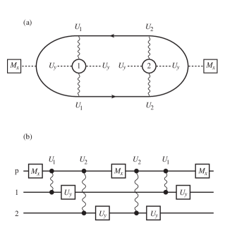
FIG. 1.: Shuttle-operation in the complete, non-demolition measurement of the Bell-aspect. Equivalent diagrams, for a traveling probe (a), and a stationary probe (b). The wiggly lines represent the interaction (18) between the probe p and the qubits. $U_{y}$ are local ${-90}^{\circ}$ qubit rotations, and $M_{x}$ are standard spin $1/2$ measurements, on the probe exclusively.

The second measurement now gives ${|\,\psi_{\text{EE}}\,\rangle}={|\,\Psi^{-}\,\rangle}$ in a fraction of the first cases equal to ${|c_{--}|}^{2}/p_{-}$. Likewise for the alternative cases. This confirms that one obtains the pure output states listed in Table I with statistical frequencies equal to

$$\sum\limits_{j}{\xi_{j}{|c_{ab}^{(j)}|}^{2}}=p_{ab}$$

G Shuttle mode

All interactions are local. It is therefore possible to operate the present procedure in shuttle mode, where the probe can travel between qubits located in different regions of space. Of course, an instantaneous measurement at space-like separation is not feasible by this method. If the rotations $U_{y}$ can be done at each qubit site, and if there is an $M_{x}$ station, then (23) can be arranged as follows

$$\cdots\underbrace{\left({U_{y}U_{2}}\right)\left({M_{x}U_{y}U_{2}}\right)}_{\text{qubit}\ 2} \cdots \underbrace{\left({U_{y}U_{1}}\right)\left({\text{init}M_{x}}\right)}_{\text{qubit}\ 1}$$

$$\cdots \underbrace{\left({U_{y}U_{1}}\right)\left({M_{x}U_{y}U_{1}}\right)}_{\text{qubit}\ 1}\cdots$$

This is represented graphically in Fig. 1.

In this shuttle procedure, both of the probe states $P_{\text{E}}$ and $P_{\text{W}}$ occur as input, and what is essential in the data is whether the probe was flipped or not. Let ‘1’ stand for a flip, and ‘0’ for no flip. There are two types of evolution, provided the shuttle action continues. Either, the state falls into ${|\,\Psi^{-}\,\rangle}$ and there are no flips of the probe. Or, there is a cyclic shift among the remaining Bell-states

$$\cdots\stackrel{{\scriptstyle 1}}{{\mapsto}}\Phi^{+}\stackrel{{\scriptstyle 1}}{{\mapsto}}\Psi^{+}\stackrel{{\scriptstyle 0}}{{\mapsto}}\Phi^{-}\stackrel{{\scriptstyle 1}}{{\mapsto}}\Phi^{+}\stackrel{{\scriptstyle 1}}{{\mapsto}}\Psi^{+}\stackrel{{\scriptstyle 0}}{{\mapsto}}\Phi^{-}\cdots$$

After the first roundtrip of the probe, provided its initial state is known, the measurement is complete. The data uniquely specifies the measurement result with respect to the input state. This is what is primarily of interest in quantum communication and teleportation.

One also knows the specific Bell-state at the output. Each output Bell-state is identified by the three most recent data items, i.e. in terms of probe flips

$$11 : \Psi^{+}$$

$$10 : \Phi^{-}$$

$$01 : \Phi^{+}$$

$$00 : \Psi^{-}$$

In this cycle, after the second roundtrip one has had the opportunity to extract any of the three alternatives. That is, after the two first probe measurements one has a pure Bell-state, and subsequently every measurement presents the next one. Therefore, the shuttle procedure may be an economical way of preparing specific Bell-states. The only statistical element remaining in this preparation procedure, even with completely arbitrary input states, for both probe and qubits, is whether the system falls into one or the other of the two cycles.

Another interesting possibility is to employ the stability of the present shuttle cycle for storage. Any perturbation, or imperfection, will be corrected after one (error-free) roundtrip (2 bits of data). With good quality in the operations $U_{1,2}$, $U_{y}$, and $M_{x}$, it would be expected that imperfections only result in recognizable glitches in otherwise perfect cycles. This would allow persistent Zeno monitoring of the Bell-state of the qubit pair. If the probe-qubit interaction is on continuously, what is required is a regularly timed sequence of ‘instantaneous’ $M_{x}U_{y}$ operations. Such a time-scale gap, apparently, seems to agree with the given conditions in some of the relevant systems.

H Cavity-field probe

Suppose a cavity mode interacts dispersively for a specific length of time with a passing Rydberg atom [53]. The resulting transformation is of the form

$$U_{1}=\exp(-i\theta\hat{n}\otimes\sigma_{z}^{(1)})$$

This interaction is suitable for the present purpose, and has the advantage that it conserves the photon number. The number operator $\hat{n}$ generates a phase-shift in the field that occupies the cavity. Thus for two qubit-atoms

$$U_{2}U_{1} = \exp(-i2\theta\hat{n}\otimes S_{z})$$

$$= 1\otimes 1$$

$$+\bigl{(}{\cos(2\theta\hat{n})-1}\bigr{)}\otimes P_{+}-i\sin(2\theta\hat{n})\otimes\sigma_{z0}P_{+}$$

$$= 1\otimes P_{-}$$

$$+\bigl{(}{\cos(2\theta\hat{n})\otimes 1-i\sin(2\theta\hat{n})\otimes\sigma_{z0}}\bigr{)}\left({1\otimes P_{+}}\right)$$

First, consider using cavity number states ${|\,0\,\rangle}$ and ${|\,1\,\rangle}$ to create phase-states [54]

$${|\,\text{E}\,\rangle}=\textstyle{1\over{\sqrt{2}}}\bigl{(}{{|\,0\,\rangle}+{|\,1\,\rangle}}\bigr{)},\quad{|\,\text{W}\,\rangle}=\textstyle{1\over{\sqrt{2}}}\bigl{(}{{|\,0\,\rangle}-{|\,1\,\rangle}}\bigr{)}$$ (24)

To achieve phase-flips between these states the interaction time must be adjusted so that $\theta=\pi/2$. This gives

$$U_{2}U_{1}=1\otimes P_{-}+(-1)^{\hat{n}}\otimes P_{+}$$ (25)

One may then consider passing the qubit-atoms through two such probe cavities in succession, with a $U_{y}$ rotation in between.

According to the Jaynes-Cummings model at exact resonance [55], the cavity field phase-states (24) can be transferred to an auxiliary probe-atom, whose state is then measured [56, 57]. The cavity can be initialized in an analogous way [58], similar to the one used in [15] to prepare entangled atom states. Another way to measure the phase in two opposite directions has been proposed in [59].

The data obtained by measuring the cavity-field phases after both atoms have passed would be analogous to those obtained with the spin $1/2$ probe. With two distinct probe systems, it is possible to postpone acquiring the data, since there is no physical interaction with the qubits involved in this. The qubit state is the mixed

$$w^{\prime\prime}_{\text{meas}}=\sum\limits_{a,b=\pm 1}{P_{ab}wP_{ab}}$$

One needs the probe data to separate the four parts in this mixture. There is no permutation of the $\Phi$ states, so by including the final $U_{yy}^{\dagger}$ one gets a clean projection on the Bell-aspect. If it is omitted, then there is a permutation corresponding to $U_{yy}$.

Next, consider starting with a coherent state of the probe field

$${|\,\alpha\,\rangle}=e^{-|\alpha|^{2}/2}\sum\limits_{n=0}^{\infty}{{{\alpha^{n}}\over{\sqrt{n!}}}{|\,n\,\rangle}}$$

where ${|\,n\,\rangle}$ are the number eigenstates, and $\alpha$ a complex number. For a qubit state ${|\,\psi\,\rangle}$ one gets

$$U_{2}U_{1}{|\,\alpha\,\rangle}\otimes{|\,\psi\,\rangle}={|\,\alpha\,\rangle}\otimes P_{-}{|\,\psi\,\rangle}+{|\,-\alpha\,\rangle}\otimes P_{+}{|\,\psi\,\rangle}$$

Although the opposite-phase coherent states are not orthogonal, their overlap decreases with field amplitude

$$\langle\alpha|-\alpha\rangle=e^{-2|\alpha|^{2}}$$

These field states resemble classical, i.e. distinct, pointer positions. Furthermore, it has been demonstrated explicitly that the coherences in the field density matrix decay in time, more rapidly for large amplitudes $|\alpha|$ [57, 60]. The time dependence appears to agree with the model [61] where the cavity field is coupled to a reservoir, which causes amplitude damping: $\alpha\exp(-\lambda t/2)$, where $\lambda$ is a coupling constant, and $t$ the time. According to this model, the ratio of off-diagonal elements to diagonal ones decreases with time as

$$\biggl{(}{{{\langle\alpha|-\alpha\rangle}\over{\langle\alpha|\alpha\rangle}}}\biggr{)}^{1-\exp(-\lambda t)}\cong e^{-2|\alpha|^{2}\lambda t},\quad\text{for}\quad\lambda t\ll 1$$

A dispersive coupling allows the qubit-atoms to interact simultaneously with the field probe. For moderately large amplitudes this could, in principle at least, take place before any significant decoherence has occurred. Subsequently, the probe measurement would be approximated by the decay of the coherences, still leaving time to read the data, before the amplitude reaches zero. Recently a model has been proposed [62] in which the field amplitude decay is prevented, although there is diffusive broadening.

III Measuring general entangled aspects

A The GHZ-aspect

Of course, eigenstates of $\sigma_{zz}$, such as ${|\,\!\uparrow\uparrow\,\rangle}$, or $\sigma_{xx}$, such as ${|\,\!\rightarrow\rightarrow\,\rangle}$, are not necessarily entangled. But the simultaneous eigenstates, the Bell-states, are. For instance

$${|\,\!\rightarrow\rightarrow\,\rangle}-{|\,\!\leftarrow\leftarrow\,\rangle}={|\,\!\uparrow\downarrow\,\rangle}+{|\,\!\downarrow\uparrow\,\rangle}$$ (26)

where ${|\,\!\rightarrow\,\rangle}$ and ${|\,\!\leftarrow\,\rangle}$ are eigenstates of $\sigma_{x}$. A three-qubit generalization of (9) therefore is

$$P_{abc}=\textstyle{1\over 8}\bigl{(}{1+a\sigma_{xxx}}\bigr{)}\bigl{(}{1+b\sigma_{zz0}}\bigr{)}\bigl{(}{1+c\sigma_{0zz}}\bigr{)}$$ (27)

with $a,b,c=\pm 1$. The partial projectors commute, since for example

$$\sigma_{xxx}\sigma_{zz0}=\sigma_{xx}\sigma_{zz}\otimes\sigma_{x}1=\sigma_{zz}\sigma_{xx}\otimes 1\sigma_{x}=\sigma_{zz0}\sigma_{xxx}$$

The 8 entangled states corresponding to $P_{ab}$ (cf. Table II) are mutually orthogonal, since at least one of the quantum numbers $a,b,c$ is different between any pair. The set will be referred to as the ‘GHZ-aspect’, since it is built to contain the original GHZ-states [17, 18, 19]

$$\textstyle{1\over{\sqrt{2}}}\bigl{(}{{|\,\!\uparrow\uparrow\uparrow\,\rangle}\pm{|\,\!\downarrow\downarrow\downarrow\,\rangle}}\bigr{)}$$

Obviously, the GHZ-basis states can be turned into each other by means of one or more unilateral spin flips, generated by $\sigma_{x}$. Measurement of this aspect was suggested for the 9-qubit error correction code [63]. These states also remain of great interest with respect to the purpose for which they were originally proposed.

Again, since one starts with just pairwise p/a tests, entanglement requires the global e/o test of the projector

$$\bar{P}_{a}=\textstyle{1\over 2}\bigl{(}{1+a\sigma_{xxx}}\bigr{)}$$ (28)

The complete, non-demolition measurement procedure for the GHZ-aspect will be presented in Sect. III D. The following is a general result, providing modules that perform partial measurements for this and other aspects.

TABLE II.: Basis states of the GHZ-aspect for three qubits. The two representations are equivalent, the second alternative using Bell-states of qubits 1 and 2, together with $\sigma_{x}$-eigenstates of qubit 3.

	$abc$	standard basis	${\mathcal{H}}^{(12)}\otimes{\mathcal{H}}^{(3)}$
1	$+++$	${|\,\!\uparrow\uparrow\uparrow\,\rangle}+{|\,\!\downarrow\downarrow\downarrow\,\rangle}$	${|\,\Phi^{+}\rightarrow\,\rangle}+{|\,\Phi^{-}\leftarrow\,\rangle}$
2	$++-$	${|\,\!\uparrow\uparrow\downarrow\,\rangle}+{|\,\!\downarrow\downarrow\uparrow\,\rangle}$	${|\,\Phi^{+}\rightarrow\,\rangle}-{|\,\Phi^{-}\leftarrow\,\rangle}$
3	$+-+$	${|\,\!\uparrow\downarrow\downarrow\,\rangle}+{|\,\!\downarrow\uparrow\uparrow\,\rangle}$	${|\,\Psi^{+}\rightarrow\,\rangle}-{|\,\Psi^{-}\leftarrow\,\rangle}$
4	$+--$	${|\,\!\uparrow\downarrow\uparrow\,\rangle}+{|\,\!\downarrow\uparrow\downarrow\,\rangle}$	${|\,\Psi^{+}\rightarrow\,\rangle}+{|\,\Psi^{-}\leftarrow\,\rangle}$
5	$-++$	${|\,\!\uparrow\uparrow\uparrow\,\rangle}-{|\,\!\downarrow\downarrow\downarrow\,\rangle}$	${|\,\Phi^{-}\rightarrow\,\rangle}+{|\,\Phi^{+}\leftarrow\,\rangle}$
6	$-+-$	${|\,\!\uparrow\uparrow\downarrow\,\rangle}-{|\,\!\downarrow\downarrow\uparrow\,\rangle}$	${|\,\Phi^{-}\rightarrow\,\rangle}-{|\,\Phi^{+}\leftarrow\,\rangle}$
7	$--+$	${|\,\!\uparrow\downarrow\downarrow\,\rangle}-{|\,\!\downarrow\uparrow\uparrow\,\rangle}$	${|\,\Psi^{-}\rightarrow\,\rangle}-{|\,\Psi^{+}\leftarrow\,\rangle}$
8	$---$	${|\,\!\uparrow\downarrow\uparrow\,\rangle}-{|\,\!\downarrow\uparrow\downarrow\,\rangle}$	${|\,\Psi^{-}\rightarrow\,\rangle}+{|\,\Psi^{+}\leftarrow\,\rangle}$

B The partial measurement module

The partial measurement corresponding to the generic projector

$$P_{a}=\textstyle{1\over 2}\bigl{(}{1+a\sigma_{z\cdots z}}\bigr{)}$$

is an operational component in a complete measurement of an $n$-qubit entangled aspect. It is convenient to label the $k$ qubits involved ($k\leq n$) sequentially as $j=1,2,\ldots,k$. The remaining $n-k$ qubits are ignored during the present procedure. For each individual qubit the quantization axis can be determined by local rotations, combined into a multilateral operation, such as $U_{y\cdots y}$. This makes the measurement suitable for testing any $k$-qubit spin correlation. In particular,

$$\bar{P}_{a}=U_{y\cdots y}^{\dagger}P_{a}U_{y\cdots y}=\textstyle{1\over 2}\bigl{(}{1+a\sigma_{x\cdots x}}\bigr{)}$$

The complete measurement of a GHZ-class entangled aspect can therefore be carried out using (essentially) only the present type of partial measurement operation.

Consider a suitable probe property, $A$, such as for instance $\sigma_{z}/2$ or $\hat{n}$. Suppose the interaction of the probe with the $j$’th qubit is

$$U_{j}=e^{-i\theta A\otimes\sigma_{z}^{(j)}}=U(\theta)\otimes P_{+}^{(j)}+U(-\theta)\otimes P_{-}^{(j)}$$ (29)

where

$$U(\theta)=e^{-i\theta A},\quad P_{\pm}^{(j)}=\textstyle{1\over 2}\bigl{(}{1\pm\sigma_{z}^{(j)}}\bigr{)}$$ (30)

As usual, $\theta$ is an adjustable angle, determined by the duration of the interaction. It is chosen (since that is adequate) to be the same for each $j$. In order to achieve a measurement it is also necessary to choose $A$, and the probe state, carefully. The probe can interact either simultaneously, or sequentially, with the $k$ qubits.

a Theorem

After these interactions the joint probe-qubit system has been transformed by the following unitary operator

$$U_{k} \cdots U_{1}$$ (31)

$$= U(\alpha_{k})\otimes U_{+}^{(1\cdots k)}P_{+}^{(1\cdots k)}+U(\beta_{k})\otimes U_{-}^{(1\cdots k)}P_{-}^{(1\cdots k)}$$ (32)

where

$$\alpha_{k}=k\textstyle{\pi\over 2},\quad\beta_{k}=\alpha_{k}-\pi$$ (33)

The operator to the left of the explicit $\otimes$ is for the probe, given by (30). Those to the right are for the $k$ qubits. The projectors are ($j=1,\cdots,k$)

$$P_{\pm}^{(1\cdots j)}=\textstyle{1\over 2}\bigl{(}{1^{(1\cdots j)}\pm\sigma_{z\cdots z}^{(1\cdots j)}}\bigr{)}$$

with notation

$$1^{(1\cdots j)} \equiv 1\otimes\cdots\otimes 1$$

$$\sigma_{z\cdots z}^{(1\cdots j)} \equiv \sigma_{z}^{(1)}\otimes\cdots\otimes\sigma_{z}^{(j)}$$

The operators $U_{\pm}$ are given by

$$U_{+}^{(1\cdots j)} = U_{+}^{(1\cdots j-1)}P_{+}^{(j)}+\eta U_{-}^{(1\cdots j-1)}P_{-}^{(j)}$$ (35)

$$U_{-}^{(1\cdots j)} = U_{+}^{(1\cdots j-1)}P_{-}^{(j)}+U_{-}^{(1\cdots j-1)}P_{+}^{(j)}$$ (36)

The recursion starts with

$$U_{+}^{(1)}=U_{-}^{(1)}=1^{(1)}$$

The projectors in these expressions are for a single qubit (the $j$’th), and $\eta$ is a phase factor to be defined in the following. Note that, if $\eta=1$ this immediately implies that (all $j=1,\cdots,k$)

$$U_{+}^{(1\cdots j)}=U_{-}^{(1\cdots j)}=1^{(1\cdots j)}$$

b Proof

The proof is by induction. As stated in (29), for the first qubit-probe interaction, $U_{1}$, the expression agrees in form with (31). Given that (31) is true for the first $j$ qubits, then

$$U_{j+1}U_{j}\cdots U_{1}$$ (37)

$$\enspace=\left\{{U(\theta)\otimes P_{+}^{(j+1)}+U(-\theta)\otimes P_{-}^{(j+1)}}\right\}$$ (38)

$$\quad\times\left\{{U(\alpha_{j})\otimes U_{+}^{(1\cdots j)}P_{+}^{(1\cdots j)}+U(\beta_{j})\otimes U_{-}^{(1\cdots j)}P_{-}^{(1\cdots j)}}\right\}$$ (39)

(qubit unit operators are not displayed). One needs the identity

$$P_{a}^{(j+1)}P_{b}^{(1\cdots j)}=P_{a}^{(j+1)}P_{ab}^{(1\cdots j+1)}$$ (40)

Here, on the left-hand side of (40)

$$\bigl{(}{1+a\sigma_{z}^{(j+1)}}\bigr{)}\bigl{(}{1+b\sigma_{z\cdots z}^{(1\cdots j)}}\bigr{)}$$

$$\enspace=1+a\sigma_{z}^{(j+1)}+b\sigma_{z\cdots z}^{(1\cdots j)}\bigl{(}{a\sigma_{z}^{(j+1)}}\bigr{)}^{2}+ab\sigma_{z\cdots z}^{(1\cdots j+1)}$$

where a unit operator has been inserted, and this agrees with the right-hand side. The four terms in (38) are then given by

$$U(\alpha_{j}+\theta) \otimes U_{+}^{(1\cdots j)}P_{+}^{(j+1)}P_{+}^{(1\cdots j+1)}$$

$$U(\beta_{j}+\theta) \otimes U_{-}^{(1\cdots j)}P_{+}^{(j+1)}P_{-}^{(1\cdots j+1)}$$

$$U(\alpha_{j}-\theta) \otimes U_{+}^{(1\cdots j)}P_{-}^{(j+1)}P_{-}^{(1\cdots j+1)}$$

$$U(\beta_{j}-\theta) \otimes U_{-}^{(1\cdots j)}P_{-}^{(j+1)}P_{+}^{(1\cdots j+1)}$$

If one takes $\theta=\pi/2$, and if (33) holds up to $j$, then the parameters in the probe $U$ are related as

$$\alpha_{j}+\textstyle{\pi\over 2} = \left({j+1}\right)\textstyle{\pi\over 2}=\alpha_{j+1}$$

$$\beta_{j}+\textstyle{\pi\over 2} = \left({j+1}\right)\textstyle{\pi\over 2}-\pi=\beta_{j+1}$$

$$\alpha_{j}-\textstyle{\pi\over 2} = \left({j+1}\right)\textstyle{\pi\over 2}-\pi=\beta_{j+1}$$

$$\beta_{j}-\textstyle{\pi\over 2} = \left({j+1}\right)\textstyle{\pi\over 2}-2\pi=\alpha_{j+1}-2\pi$$

The last can give rise to a phase factor

$$\eta=U(-2\pi)=e^{i2\pi A}$$

The measurement design requires this to be a number for all relevant probe states. Evidently, in order to obtain a measurement transformation, there has to be restrictions of some kind, else one would have just any transformation. For $A=\sigma_{z}/2$ one has $\eta=-1$, and for $A=\hat{n}$ one has $\eta=1$. If this condition (that $\eta$ be a number) is satisfied, then the proof is complete.

c Check

With a spin $1/2$ probe and $k=2$ one gets

$$\alpha_{2}=\pi,\quad\beta_{2}=0$$

and

$$U_{+}^{(12)} = U_{+}^{(1)}P_{+}^{(2)}-U_{-}^{(1)}P_{-}^{(2)}=P_{+}^{(2)}-P_{-}^{(2)}=\sigma_{z}^{(2)}$$

$$U_{-}^{(12)} = P_{-}^{(2)}+P_{+}^{(2)}=1$$

So

$$U_{2}U_{1}=U(\pi)\otimes\sigma_{z}^{(2)}P_{+}^{(12)}+U(0)\otimes P_{-}^{(12)}$$

in agreement with (18).

Since the probe advances, or retreats, by $\pi/2$ in each encounter with a qubit, all the four compass states (12) can occur. One gets

$$\rho^{\prime} = U_{k}\cdots U_{1}\,v\otimes w\,U_{1}^{\dagger}\cdots U_{k}^{\dagger}$$

$$= U(\alpha_{k})\,v\,U(\alpha_{k})^{\dagger}\otimes U_{+}^{(1\cdots k)}P_{+}^{(1\cdots k)}w\,P_{+}^{(1\cdots k)}{U_{+}^{(1\cdots k)}}^{\dagger}$$

$$+U(\alpha_{k})\,v\,U(\beta_{k})^{\dagger}\otimes U_{+}^{(1\cdots k)}P_{+}^{(1\cdots k)}w\,P_{-}^{(1\cdots k)}{U_{-}^{(1\cdots k)}}^{\dagger}$$

$$+\cdots$$

With even $k$ one must measure the probe in the x-direction, using $M_{x}$. For odd $k$ in the y-direction. Of course, one can then consider rotating the probe by $\pi/2$, in order to be able to use the $M_{x}$ equipment repeatedly.

For example, with even $k$, starting with $v=P_{\text{E}}$, after the probe has been measured, off-diagonal terms in the probe part of $\rho^{\prime}_{\text{meas}}$ are of the form

$$P_{E,W}U(\alpha_{k})P_{\text{E}}U(\alpha_{k}-\pi)^{\dagger}P_{E,W}$$

They will vanish due to the extra rotation by $\pi$, provided the relevant probe states are orthogonal (by design). Likewise, the diagonal terms are

$$P_{E,W}U(\alpha_{k})P_{\text{E}}U(\alpha_{k})^{\dagger}P_{E,W}$$

and

$$P_{W,E}U(\alpha_{k}-\pi)P_{\text{E}}U(\alpha_{k}-\pi)^{\dagger}P_{W,E}$$

If $k=2s$, and $s=1,3,\ldots$, then the probe state in the first term is $P_{\text{W}}$, while in the second term it is $P_{\text{E}}$, and conversely if $s$ is even. There remains (odd $s$)

$$\rho^{\prime}_{\text{meas}} = P_{\text{W}}\otimes U_{+}^{(1\cdots k)}P_{+}^{(1\cdots k)}w\,P_{+}^{(1\cdots k)}{U_{+}^{(1\cdots k)}}^{\dagger}$$

$$+P_{\text{E}}\otimes U_{-}^{(1\cdots k)}P_{-}^{(1\cdots k)}w\,P_{-}^{(1\cdots k)}{U_{-}^{(1\cdots k)}}^{\dagger}$$

and so forth.

TABLE III.: GHZ-state propagation during the uncompensated measurement according to (27)(overall phase omitted). The probe starts in ${|\,E\,\rangle}$. Numbers refer to the listing in Table II, letters to the four compass states (12) of a qubit probe.

input	$U_{2}U_{1}$	$M_{x}$	$U_{2}U_{3}$	$M_{x}$	$\bar{U}_{3}\bar{U}_{2}\bar{U}_{1}$	$M_{y}$
1	5	W	1	E	${|\,\Psi^{+}\rightarrow\,\rangle}-{|\,\Phi^{-}\leftarrow\,\rangle}$	S
2	6	W	6	W	${|\,\Phi^{-}\rightarrow\,\rangle}-{|\,\Psi^{+}\leftarrow\,\rangle}$	S
3	3	E	7	W	${|\,\Psi^{-}\rightarrow\,\rangle}-{|\,\Phi^{+}\leftarrow\,\rangle}$	S
4	4	E	4	E	${|\,\Phi^{+}\rightarrow\,\rangle}-{|\,\Psi^{-}\leftarrow\,\rangle}$	S
5	1	W	5	E	${|\,\Phi^{-}\rightarrow\,\rangle}+{|\,\Psi^{+}\leftarrow\,\rangle}$	N
6	2	W	2	W	${|\,\Psi^{+}\rightarrow\,\rangle}+{|\,\Phi^{-}\leftarrow\,\rangle}$	N
7	7	E	3	W	${|\,\Phi^{+}\rightarrow\,\rangle}+{|\,\Psi^{-}\leftarrow\,\rangle}$	N
8	8	E	8	E	${|\,\Psi^{-}\rightarrow\,\rangle}+{|\,\Phi^{+}\leftarrow\,\rangle}$	N

C Compensation

Besides projections by $P_{\pm}$, the $k$-qubit system may experience some unitary transformations, as when $\eta=-1$ for the qubit probe. One has

$$U_{+}^{(1\cdots k)}{U_{+}^{(1\cdots k)}}^{\dagger} = U_{+}^{(1\cdots k-1)}{U_{+}^{(1\cdots k-1)}}^{\dagger}P_{+}^{(k)}$$

$$+{|\eta|}^{2}\,U_{-}^{(1\cdots k-1)}{U_{-}^{(1\cdots k-1)}}^{\dagger}P_{-}^{(k)}$$

$$= P_{+}^{(k)}+P_{-}^{(k)}=1$$

using the recursion (35), and likewise for $U_{-}$. It also follows that $U_{\pm}$ and $P_{\pm}$ commute. The unitary operators $U_{\pm}$ are Hermitean, by recursive construction. Consequently

$${\bigl{(}{U_{\pm}^{(1\cdots k)}}\bigr{)}}^{2}=1^{(1\cdots k)}$$

Therefore, if the unitary transformations $U_{\pm}$ on the selected $k$ qubits are not desirable, a clean projection can be obtained by repeating the measurement, as described already for the Bell-aspect in (22).

For the qubit probe case, there is an alternative way to compensate the unitary operations. For the $k$ qubits, let

$$U_{z\cdots z}^{(1\cdots k)}=U_{z}^{(1)}\otimes\cdots\otimes U_{z}^{(k)}$$

where

$$U_{z}=e^{-i{\textstyle{\pi\over 2}}\sigma_{z}/2}=\textstyle{1\over{\sqrt{2}}}\bigl{(}{1-i\sigma_{z}}\bigr{)}$$

This represents a multilateral $+\pi/2$ rotation about the z-axis. Then it is straightforward to show that

$$\enspace U_{z\cdots z}^{(1\cdots k)}U_{k}\cdots U_{1}$$ (41)

$$\quad=U(\alpha_{k})\otimes g^{k}P_{+}^{(1\cdots k)}+U(\beta_{k})\otimes ig^{k}P_{-}^{(1\cdots k)}$$ (42)

with

$$g=e^{-i\pi/4}=\textstyle{1\over{\sqrt{2}}}\left({1-i}\right)$$

For instance, one has

$$U_{z}P_{+}=gP_{+},\quad U_{z}P_{-}=igP_{-}$$

Another way is to write

$$\tilde{U}_{j}=U_{z}^{(j)}U_{j}=e^{-i\theta{\textstyle{1\over 2}}(1+\sigma_{z})\otimes\sigma_{z}^{(j)}}$$

and use it for $\theta=\pi/2$ as before, but with $A=P_{+}$ for the probe, i.e.

$$\tilde{U}(\theta)=e^{-i\theta P_{+}}=1+\left({e^{-i\theta}-1}\right)P_{+}$$

This gives $\eta=\tilde{U}(-2\pi)=1$. In the expression (31) one must then use $U_{\pm}=1$, together with

$$\tilde{U}(\alpha_{k}) = e^{-ik{\textstyle{\pi\over 2}}P_{+}}=g^{k}U(\alpha_{k})$$

$$\tilde{U}(\beta_{k}) = e^{-i(k-2){\textstyle{\pi\over 2}}P_{+}}=ig^{k}U(\beta_{k})$$

Apart from the phase factors, the present global rotation compensates as effectively as repeating the measurement, although it requires a different set of operations from what is otherwise used, i.e. the $U_{z}$. In some systems, this rotation could perhaps be drawn from an inherent ‘precession’ of the qubits (not included here).

D Shuttle-measurement of the GHZ-states

Entangled states with a structure such as the one shown in (27) for the eight GHZ-basis states can be measured in a complete, non-demolition fashion by means of the partial measurement module just established. Of course, these modules can also be used separately in ways, which need not imply entanglement. In each stage, there are options to repeat or to compensate, as described above in Sect. III C. For the following design, it will be regarded as acceptable that there are simple cycles between the members of the GHZ-basis.

TABLE IV.: GHZ-state propagation during two rounds of shuttle operation (overall phase omitted). The probe starts (and ends) in ${|\,E\,\rangle}$. Numbers refer to the listing in Table II.

input	first-round data	output	second-round data
1	WESW	5	EWSE
2	WWSE	2	WWSE
3	EWSE	3	EWSE
4	EESW	8	WWSE
5	WENW	1	EWNE
6	WWNE	6	WWNE
7	EWNE	7	EWNE
8	EENW	4	WWNE

The probe is initialized in the state $P_{\text{E}}$. It first interacts with qubits 1 and 2, by $U_{1}$ and $U_{2}$, and is then measured in the x-direction, $M_{x}$. Secondly, it interacts with qubit 3 and again with qubit 2, via $U_{3}$ and $U_{2}$. It is then measured again with $M_{x}$. When the GHZ-basis states are given as input, this non-demolition processing leads to some permutations, as listed in Table III. They come from

$$U_{+}^{(12)} = P_{+}^{(2)}-P_{-}^{(2)}=\sigma_{z}^{(2)},\quad U_{-}^{(12)}=P_{-}^{(2)}+P_{+}^{(2)}=1$$

$$U_{+}^{(32)} = P_{+}^{(2)}-P_{-}^{(2)}=\sigma_{z}^{(2)},\quad U_{-}^{(32)}=P_{-}^{(2)}+P_{+}^{(2)}=1$$

The pattern of probe data (2 bits) now allows to distinguish four orthogonal subspaces, but there is not yet any certainty of entanglement.

The e/o test starts by tilting each qubit spin by means of $U_{y}$. Then all qubits interact with the probe. Returning the qubits by $U_{y}^{\dagger}$, all in all (overbars indicate that the operators are built from $\sigma_{x}$ instead of $\sigma_{z}$)

$$\bar{U}_{3}\bar{U}_{2}\bar{U}_{1} = U_{yyy}^{\dagger}U_{3}U_{2}U_{1}U_{yyy}$$

$$= \left({U_{y}^{\dagger}U_{3}U_{y}}\right)\left({U_{y}^{\dagger}U_{2}U_{y}}\right)\left({U_{y}^{\dagger}U_{1}U_{y}}\right)$$

Finally the probe is measured in the y-direction, $M_{y}$. Or, it is rotated by $-\pi/2$, say, and measured with the $M_{x}$ equipment (this option will not be included here). According to (31) the interactions produce

$$\bar{U}_{3}\bar{U}_{2}\bar{U}_{1}$$

$$\enspace=U(3\pi/2)\otimes\bar{U}_{+}^{(123)}\bar{P}_{+}^{(123)}+U(\pi/2)\otimes\bar{U}_{-}^{(123)}\bar{P}_{-}^{(123)}$$

Here

$$\bar{P}_{\pm}^{(123)}=\textstyle{1\over 2}\bigl{(}{1^{(123)}\pm\sigma_{xxx}^{(123)}}\bigr{)}$$

As the probe starts in $P_{\text{E}}$, say, when operating on the GHZ-states it will become either $P_{\text{N}}$ or $P_{\text{S}}$, depending on the outcome of the e/o test, and hence must be measured in the y-direction. With $\eta=-1$, the unitary operators are

$$\bar{U}_{+}^{(123)}=\sigma_{x}^{(2)}\bar{P}_{+}^{(3)}-\bar{P}_{-}^{(3)},\quad\bar{U}_{-}^{(123)}=\sigma_{x}^{(2)}\bar{P}_{-}^{(3)}+\bar{P}_{+}^{(3)}$$

These determine which 3-qubit states are available after completion of the measurement. Use the following representation

$${|\,\Psi\rightarrow\,\rangle}^{(123)}\equiv{|\,\Psi\,\rangle}^{(12)}\otimes{|\,\rightarrow\,\rangle}^{(3)}$$

The first factor in the right-hand expression stands for any of the Bell-states, so

$$\sigma_{0x}{|\,\Psi^{\pm}\,\rangle}={|\,\Phi^{\pm}\,\rangle},\quad\sigma_{0x}{|\,\Phi^{\pm}\,\rangle}={|\,\Psi^{\pm}\,\rangle}$$

and the last factor is a $\sigma_{x}$ eigenstate. The GHZ-basis in this representation is shown in Table II. As usual, the even states 1 to 4 are operated upon by $\bar{U}_{+}$, while the probe turns $3\pi/2$, and the odd states 5 to 8 by $\bar{U}_{-}$, the probe turning $\pi/2$.

The resulting qubit output states and probe data are listed in Table III. It depends, of course, on the circumstances, whether these output states are useful. In any event, there is a compensation procedure using only local rotations, $U_{z}$, which will produce output within the original GHZ-aspect. Another such alternative output-aspect is entered if one omits the final $U_{yyy}^{\dagger}$.

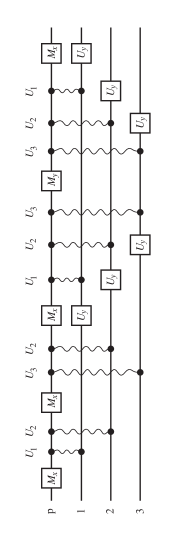
FIG. 2.: Shuttle-operation of the complete, non-demolition measurement of the GHZ-aspect. The probe p interacts with qubits 1, 2, and 3 via (29) (wiggly lines) and is measured in the x- and y-directions at the standard measuring stations $M_{x}$ and $M_{y}$. The qubits are rotated by local $U_{y}$. The GHZ-states pass unhindered, except for some permutations.

Repeating the last partial measurement corresponds to doing

$$\left({M_{x}\bar{U}_{1}\bar{U}_{2}\bar{U}_{3}}\right)\left({M_{y}\bar{U}_{3}\bar{U}_{2}\bar{U}_{1}}\right)$$

$$\enspace=\left({M_{x}U_{yyy}^{\dagger}U_{1}U_{2}U_{3}U_{yyy}}\right)\left({M_{y}U_{yyy}^{\dagger}U_{3}U_{2}U_{1}U_{yyy}}\right)$$

According to Sect. III C, this will return the appropriate GHZ-states, i.e. the ones that are present after the first two stages in Table III.

This allows the following shuttle design. Cancel the intermediate rotations by the unitarity of $U_{yyy}$. At the end, add $U_{yyy}^{2}=-i\sigma_{yyy}$, which merely performs another permutation on the GHZ-basis (exchanging the even and odd states, i.e. (15)(26)(37)(48) apart from phase factors $\pm 1$). This gives the shuttle procedure of Fig. 2

$$\left({M_{x}U_{yyy}U_{1}U_{2}U_{3}}\right)\left({M_{y}U_{3}U_{2}U_{1}U_{yyy}}\right)$$

The final output is shown in Table IV. One must of course do the third probe measurement, $M_{y}$, in order to complete the projection of the qubit system into one-dimensional subspaces. The aspect at this stage is not GHZ. The data from the fourth probe measurement, $M_{x}$, is redundant, but a useful check on the e/o test. The unitary operations preceding it produce the GHZ output-states listed.

Having returned to the GHZ-aspect, the measurement sequence can now be repeated. Apart from phase-factors, this merely gives rise to the simple cycles

$$\cdots 1\mapsto 5\mapsto 1\cdots,\quad\cdots 4\mapsto 8\mapsto 4\cdots$$

After two rounds, therefore, all the GHZ-basis states emerge in the original places, and the probe is in $P_{\text{E}}$, where it started. The GHZ-states also result when the input is an arbitrary mixed state, $w$, with statistical frequencies equal to the predicted probabilities for $w$. One can recognize the outcome of the complete, non-demolition measurement by the probe data sequence that has been recorded. For two rounds, as shown in Table IV, only eight 8-bit words out of a total of 256 possible ones correspond to an error-free measurement. These words are going to repeat as the shuttle continues running.

IV Conclusions

The measurement procedure established in the present paper is different from the existing ones in at least one of the following respects: (a) It is a complete, non-demolition measurement process, under which all the entangled basis states are invariant. (b) The entire interaction with the entangled system is taken care of by a single (qubit) probe, used repeatedly. (c) There is no interaction between the individual parts of the entangled system. (d) There is no interaction between the environment and the entangled system, only with the probe. (e) All interactions are two-qubit interactions between the probe and each of the constituents of the entangled system in turn. (f) This interaction is of the simplest conceivable form, and only one kind of probe-qubit interaction is required to perform the entire measurement. (g) The design is modular, so that it can perform partial measurements, and can be extended to handle entangled states of many qubits. (h) The same procedure can be adjusted to measure a wide range of different entangled states by local qubit operations, such as unilateral spin rotations.

Apart from this one needs external apparatus, which can perform measurements on the probe. It is not essential how the apparatus is built, as long as it performs a standard measurement, say measures the probe spin in the x-direction. This equipment can also be localized, i.e. it does not require entangled states of the apparatus to be prepared and distributed beforehand.

With the present procedure the measurement process is split up into exclusively local operations and interactions, which can take place sequentially as the probe visits each of the qubit components in turn. All these operations are elementary, and in their totality they can be said to define the operational nature of the observable entanglement.

It is possible to design the probe schedule in a shuttle mode, which may be repeated indefinitely. In this way one can take advantage of the quantum Zeno effect to maintain the entangled states for a length of time, with an insignificant probability of decoherence. Such a device would be capable, in principle at least, to store entangled states until they are released at a predictable time, in a predictable state. The shuttle process is stable, and self-correcting, in the sense that any random errors are removed after a few steps by the probe measurement actions.

REFERENCES

• [1] Electronic address: ularsen@nbi.dk
• [2] J. A. Wheeler and W. H. Zurek, Quantum Theory and Measurement (Princeton U. P., Princeton, N. J., 1983).
• [3] J. S. Bell, Speakable and unspeakable in quantum mechanics (Cambridge U. P., Cambridge, 1987).
• [4] A. Aspect, J. Dalibard, and G. Roger, Phys. Rev. Lett. 47, 1804 (1982).
• [5] W. Tittel, J. Brendel, H. Zbinden, and N. Gisin, Phys. Rev. Lett. 81, 3563 (1998).
• [6] G. Weihs, T. Jennewein, C. Simon, H. Weinfurter, and A. Zeilinger, LANL e-print archive, quant-ph/9810080.
• [7] S. J. D. Phoenix and S. M. Barnett, J. Mod. Optics 40, 979 (1993).
• [8] M. Zukowski, A. Zeilinger, M. A. Horne, and A. K. Ekert, Phys. Rev. Lett. 71, 4287 (1993).
• [9] J. I. Cirac and P. Zoller, Phys. Rev. A 50, R2799 (1994).
• [10] C. C. Gerry, Phys. Rev. A 53, 2857 (1996).
• [11] A. Zeilinger, M. A. Horne, H. Weinfurter, and M. Zukowski, Phys. Rev. Lett. 78, 3031 (1997).
• [12] S. Bose, V. Vedral, and P. L. Knight, Phys. Rev. A 57, 822 (1998).
• [13] S. L. Braunstein, A. Mann, and M. Revzen, Phys. Rev. Lett. 68, 3259 (1992).
• [14] P. G. Kwiat, K. Mattle, H. Weinfurter, A. Zeilinger, A. V. Sergienko, and Y. Shih, Phys. Rev. Lett. 75, 4337 (1995).
• [15] E. Hagley, X. Maitre, G. Nogues, C. Wunderlich, M. Brune, J. M. Raimond, and S. Haroche, Phys. Rev. Lett. 79, 1 (1997).
• [16] Q. A. Turchette, C. S. Wood, B. E. King, C. J. Myatt, D. Leibfried, W. M. Itano, C. Monroe, and D. J. Wineland, LANL e-print archive, quant-ph/9806012.
• [17] D. M. Greenberger, M. A. Horne, and A. Zeilinger, in Bell’s Theorem, Quantum Theory and Conceptions of the Universe, edited by M. Kafatos (Kluwer, Dordrecht, 1989), pp. 69–72.
• [18] D. M. Greenberger, M. A. Horne, A. Shimony, and A. Zeilinger, Am. J. Phys. 58, 1131 (1990).
• [19] N. D. Mermin, Am. J. Phys. 58, 731 (1990).
• [20] D. Bouwmeester, J.-W. Pan, M. Daniell, H. Weinfurter, and A. Zeilinger, LANL e-print archive, quant-ph/9810035.
• [21] R. Laflamme, E. Knill, W. H. Zurek, P. Catasti, and S. V. S. Mariappan, Phil. Trans. R. Soc. Lond. A 356, 1941 (1998).
• [22] K. Mattle, H. Weinfurter, P. G. Kwiat, and A. Zeilinger, Phys. Rev. Lett. 76, 4656 (1996).
• [23] C. Monroe, D. M. Meekhof, B. E. King, W. M. Itano, and D. J. Wineland, Phys. Rev. Lett. 75, 4714 (1995).
• [24] Q. A. Turchette, C. J. Hood, W. Lange, H. Mabuchi, and H. J. Kimble, Phys. Rev. Lett. 75, 4710 (1995).
• [25] J. A. Jones and M. Mosca, J. Chem. Phys. 109, 1648 (1998).
• [26] J. A. Jones, M. Mosca, and R. Hvass Hansen, Nature 393, 344 (1998).
• [27] I. L. Chuang, N. Gershenfeld, and M. Kubinec, Phys. Rev. Lett. 80, 3408 (1998).
• [28] I. L. Chuang, L. M. K. Vandersypen, X. Zhou, D. W. Leung, and S. Lloyd, Nature 393, 143 (1998).
• [29] D. G. Cory, M. D. Price, W. Maas, E. Knill, R. Laflamme, W. H. Zurek, T. F. Havel, and S. S. Somaroo, Phys. Rev. Lett. 81, 2152 (1998).
• [30] D. Bouwmeester, J.-W. Pan, K. Mattle, M. Eibl, H. Weinfurter, and A. Zeilinger, Nature 390, 575 (1997).
• [31] D. Boschi, S. Branca, F. De Martini, L. Hardy, and S. Popescu, Phys. Rev. Lett. 80, 1121 (1998).
• [32] J.-W. Pan, D. Bouwmeester, H. Weinfurter, and A. Zeilinger, Phys. Rev. Lett. 80, 3891 (1998).
• [33] A. Furusawa, J. L. Sørensen, S. L. Braunstein, C. A. Fuchs, H. J. Kimble, and E. S. Polzik, Science 282, 706 (1998).
• [34] M. A. Nielsen, E. Knill, and R. Laflamme, Nature 396, 52 (1998).
• [35] C. H. Bennett and S. J. Wiesner, Phys. Rev. Lett. 69, 2881 (1992).
• [36] C. H. Bennett, G. Brassard, C. Crépeau, R. Jozsa, A. Peres, and W. K. Wootters, Phys. Rev. Lett. 70, 1895 (1993).
• [37] L. Vaidman, Phys. Rev. A 49, 1473 (1994).
• [38] S. L. Braunstein and H. J. Kimble, Phys. Rev. Lett. 80, 869 (1998).
• [39] H. Weinfurter, Europhys. Lett. 25, 559 (1994).
• [40] A. Zeilinger, H. J. Bernstein, and M. A. Horne, J. Mod. Optics 41, 2375 (1994).
• [41] S. L. Braunstein and A. Mann, Phys. Rev. A 51, R1727 (1995).
• [42] M. Michler, K. Mattle, H. Weinfurter, and A. Zeilinger, Phys. Rev. A 53, R1209 (1996).
• [43] J.-W. Pan and A. Zeilinger, Phys. Rev. A 57, 2208 (1998).
• [44] L. Vaidman and N. Yoran, LANL e-print archive, quant-ph/9808040.
• [45] N. Lütkenhaus, J. Calsamiglia, and K.-A. Suominen, LANL e-print archive, quant-ph/9809063.
• [46] S. Popescu, LANL e-print archive, quant-ph/9501020.
• [47] A. Barenco, D. Deutsch, A. Ekert, and R. Jozsa, Phys. Rev. Lett. 74, 4083 (1995).
• [48] D. Bruss, A. Ekert, S. F. Huelga, J.-W. Pan, and A. Zeilinger, Phil. Trans. R. Soc. Lond. A 355, 2259 (1997).
• [49] Y. Aharonov, D. Albert, and L. Vaidman, Phys. Rev. D 34, 1805 (1986).
• [50] J. F. Clauser, M. A. Horne, A. Shimony, and R. A. Holt, Phys. Rev. Lett. 23, 880 (1969).
• [51] U. Larsen, J. Phys. A 23, 1041 (1990).
• [52] U. Larsen, J. Phys. A 21, 4513 (1988).
• [53] M. Brune, S. Haroche, J. M. Raimond, L. Davidovich, and N. Zagury, Phys. Rev. A 45, 5193 (1992).
• [54] D. T. Pegg and S. M. Barnett, Phys. Rev. A 39, 1665 (1989).
• [55] M. O. Scully and M. S. Zubairy, Quantum Optics (Cambridge U. P., Cambridge, 1997).
• [56] S. Haroche, Ann. N. Y. Acad. Sci. 755, 73 (1995).
• [57] M. Brune, E. Hagley, J. Dreyer, X. Maitre, A. Maali, C. Wunderlich, J. M. Raimond, and S. Haroche, Phys. Rev. Lett. 77, 4887 (1996).
• [58] K. Vogel, V. M. Akulin, and W. P. Schleich, Phys. Rev. Lett. 71, 1816 (1993).
• [59] S. M. Barnett and D. T. Pegg, Phys. Rev. Lett. 76, 4148 (1996).
• [60] L. Davidovich, M. Brune, J. M. Raimond, and S. Haroche, Phys. Rev. A 53, 1295 (1996).
• [61] D. F. Walls and G. J. Milburn, Phys. Rev. A 31, 2403 (1985).
• [62] G. S. Agarwal, LANL e-print archive, quant-ph/9810052.
• [63] P. W. Shor, Phys. Rev. A 52, R2493 (1995).