Validity of Feynman’s prescription of disregarding the Pauli principle
in intermediate states

Abstract

Regarding the Pauli principle in quantum field theory and in many-body quantum mechanics, Feynman advocated that Pauli’s exclusion principle can be completely ignored in intermediate states of perturbation theory. He observed that all virtual processes (of the same order) that violate the Pauli principle cancel out. Feynman accordingly introduced a prescription, which is to disregard the Pauli principle in all intermediate processes. This ingeneous trick is of crucial importance in the Feynman diagram technique. We show, however, an example in which Feynman’s prescription fails. This casts doubts on the general validity of Feynman’s prescription.

]

I Introduction

In his space-time approach to quantum electrodynamics, Feynman advocated: “It is obviously simpler to disregard the exclusion principle completely in the intermediate states” [1]. He examined processes involving several particles and observed that all virtual processes that violate Pauli’s exclusion principle (formally) cancel out. It is understood that all virtual processes of the same orders are taken into account. On the basis of this observation Feynman introduced a prescription that is to disregard the Pauli principle in all intermediate states. This ingenious trick was crucial in accomplishing the enormous simplification and transparency of perturbation theory. For example, the vacuum polarization can be related to Feynman diagrams with an electron loop or loops. Although the process represented by a loop diagram may (at least partially) violate Pauli’s exclusion principle, no restriction needs to be imposed on integrations with respect to associated momentum variables. Feynman’s prescription is also often used in perturbation calculations for many-body systems in quantum mechanics.

Various aspects of Feynman’s prescription have been discussed by several authors [2]. There are some intriguing implications regarding the meson effects in nuclei or nuclear matter. Feynman’s prescription is instrumental in proving Goldstone’s theorem for many-body systems. We are not going to review these topics in this paper but we emphasize that no suspicion seems to have ever been raised in the literature against the validity of Feynman’s prescription.

The purpose of this paper we present an example that casts doubt about the general validity of Feynman’s prescription. The example is concerned with the second order energy shift of a relativistic bound system. We consider a model that consists of a particle bound in a given potential. The wave function of the particle is subject to the Dirac equation with the given binding potential. In addition to the bound particle, there is a vacuum background. It is understood that the vacuum background is an integral part of the bound system. When an external perturbation is applied, the energy of the system is shifted. We calculate the energy shift in second order perturbation theory. We are particularly interested in the vacuum effect to which the Pauli principle is relevant.

We consider two methods, I and II, for calculating the energy shift. In method I we take account of the Pauli principle whenever it is applicable. In method II we disregard the Pauli principle altogether. We confirm that these two methods formally agree. This illustrates Feynman’s prescription. When methods I and II are explicitly worked out for the example, however, the results of the two methods turn out to disagree with each other. We analyze the intriguing mechanism of this discrepancy.

In Sec. II we set up the model and illustrate Feynman’s prescription. In Sec. III we make the model more explicit. We consider a charged particle that is bound in an infinite square-well potential of the Lorentz scalar type. This is a one-dimensional version of the “bag model”. For the external perturbation we assume a homogeneous electric field. Then the second order energy shift is related to the electric polarizability of the system. We carry out the calculations of methods I and II. The two methods result in different energy shifts (and hence different values of the electric polarizability). We analyze the source of the discrepancy. In Sec. IV we confirm the result of method II by repeating the calculation by using the Dalgarno-Lewis (DL) method [3, 4, 5]. A summary and discussions are given in Sec. V. Some details concerning the series that appear in method II are relegated to the Appendix.

II Feynman’s prescription

As a way of setting up notation, let us start with a problem of single-particle quantum mechanics. Let the Hamiltonian of the model be

$$H=H_{0}+V\,,$$ (1)

where $H_{0}$ is the Dirac Hamiltonian with a binding potential and $V$ is the external perturbation. (Imagine something like a hydrogen atom, with Hamiltonian $H_{0}$, placed in a weak external electric field $V$. Assume that the proton is merely a source of the Coulomb potential that binds the electron of the atom.) We take $H_{0}$ as the unperturbed Hamiltonian and treat $V$ by perturbation theory. It is understood that the solutions of the Dirac equation with $H_{0}$ are known for all stationary states,

$$H_{0}|i\rangle=\epsilon_{i}|i\rangle\,,\hskip 21.68121ptH_{0}|-j\rangle=\epsilon_{-j}|-j\rangle\,,$$ (2)

where $i=1,2,\cdots$ and $-j=-1,-2,\cdots$ . The $|i\rangle$’s are positive energy states with $\epsilon_{i}>0$ and $|-j\rangle$’s are negative energy states with $\epsilon_{-j}<0$. In particular $|1\rangle$ is the lowest positive energy state (like the 1$S$-state of the hydrogen atom). We are assuming that the eigenvalues are all discrete. (It is not difficult to include continuum states; see Sec. V.) The $|i\rangle$’s and $|-j\rangle$’s form a complete orthonormal basis set. Figure 1 schematically shows the unperturbed energy spectrum.

FIG. 1.: Unperturbed energy levels defined by Eq. (2). The dots indicate occupied states.

For the unperturbed state let us take $|1\rangle$, the state of the lowest positive energy [6]. In single-particle quantum mechanics we do not consider the vacuum background. In other words, we assume that the negative energy states are all empty. In this sense let us momentarily ignore the dots of the states of the $|-j\rangle$’s in Fig. 1. Then the energy shift $W_{\rm QM}$ of state $|1\rangle$ caused by perturbation $V$ is given by

$$W_{\rm QM}=\sum_{i\neq 1}\frac{|V_{i,1}|^{2}}{\epsilon_{1}-\epsilon_{i}}+\sum_{j}\frac{|V_{-j,1}|^{2}}{\epsilon_{1}-\epsilon_{-j}}\,,$$ (3)

where $V_{i,1}\equiv\langle i|V|1\rangle$ and $V_{-j,1}\equiv\langle-j|V|1\rangle$. Suffix QM refers to single-particle quantum mechanics. The summation for $i$ ($j$) is for the positive (negative) energy intermediate states.

Let us now take account of the vacuum background that accompanies the particle bound in $|1\rangle$. Let us examine the vacuum from the point of view of Dirac’s hole theory. The vacuum consists of an infinite number of particles that occupy all of the negative energy states as indicated with dots in Fig. 1. Before the external perturbation $V$ is applied, the negative energy states are eigenstates of $H_{0}$. The energy of the unperturbed system, including the vacuum background, is

$$E=\epsilon_{1}+\sum_{j}\epsilon_{-j}\,.$$ (4)

The sum over the negative energy states is the energy of the vacuum. This vacuum is different from the “free vacuum”. The $\epsilon_{j}$’s are eigenvalues of $H_{0}$ that contains the binding interaction. The summation of Eq. (4) diverges but this is not a serious problem. If we subtract the energy of the free vacuum, the summation will converge but let us not delve into this aspect. We are only interested in the energy shift rather than the energy itself. All $\epsilon$’s and hence the total energy $E$ are shifted by external perturbation $V$. Let us examine two methods, I and II, for calculating the energy shift.

Method I. In this method we take account of the Pauli principle in intermediate states. Energy $\epsilon_{1}$ is shifted by

$$W_{1}=\sum_{i\neq 1}\frac{|V_{i,1}|^{2}}{\epsilon_{1}-\epsilon_{i}}\,,$$ (5)

where the Pauli principle excludes the negative energy states as intermediate states. The difference between $W_{1}$ and $W_{\rm QM}$ is due to the presence of the vacuum background in the former. On the other hand the vacuum energy itself also shifts by

$$W_{\rm vac}=\sum_{j}W_{-j}\,,\hskip 8.5359ptW_{-j}=\sum_{i\neq 1}\frac{|V_{i,-j}|^{2}}{\epsilon_{-j}-\epsilon_{i}}$$ (6)

Again the summation over $i$ $(j)$ is for positive (negative) energy states. The intermediate state of $i=1$ is excluded because it is already occupied. Then the total energy shift of the system, including the vacuum background, is given by

$$W=W_{1}+W_{\rm vac}\,.$$ (7)

The $W_{1}$ and $W_{\rm vac}$ are both negative and hence $W$ is negative. Note that $W_{\rm QM}$ can be positive because of the contributions from the negative energy intermediate states.

Method II. In this method we disregard the Pauli principle in all intermediate states. We can rewrite the above $W$ by adding and subtracting the same terms as

$$W^{\prime}=W^{\prime}_{1}+W^{\prime}_{\rm vac},\hskip 8.5359ptW^{\prime}_{1}=W_{\rm QM}\,,$$ (8)

$$W^{\prime}_{\rm vac}=\sum_{j}W^{\prime}_{-j}\,,\hskip 5.69046ptW^{\prime}_{-j}=\sum_{i}\frac{|V_{i,-j}|^{2}}{\epsilon_{-j}-\epsilon_{i}}+\sum_{k\neq j}\frac{|V_{-k,-j}|^{2}}{\epsilon_{-j}-\epsilon_{-k}}\,,$$ (9)

where $|-k\rangle$’s are also negative energy unperturbed states [7, 8]. The restriction $i\neq 1$ has been removed in the $i$-summation for $W^{\prime}_{-j}$. Each of $W^{\prime}_{1}$ and $W^{\prime}_{-j}$ is the energy shift in the context of single-particle quantum mechanics. The $W^{\prime}_{\rm vac}$ is the vacuum energy in the absence of the particle in $|1\rangle$. The $W^{\prime}_{1}$ and $W^{\prime}_{\rm vac}$ both contain terms that violate the Pauli principle but such terms all cancel out when they are added to obtain $W^{\prime}$. Note also that the effects of transitions between negative energy states cancel out,

$$\sum_{j}\sum_{k\neq j}\frac{|V_{-k,-j}|^{2}}{\epsilon_{-j}-\epsilon_{-k}}=0\,.$$ (10)

The formal equality between $W$ of Eq. (7) and $W^{\prime}$ of Eq. (8) illustrates Feynman’s prescription [1]. Let us warn, however, that this equivalence relies on the convergence of the series involved, in particular, the $j$-summation of $W^{\prime}_{\rm vac}$ of Eq. (9) that involves Eq. (10).

In quantum field theory no negative-energy particles appear but antiparticles of positive energies appear instead. The unperturbed state that we consider is ${c_{1}}^{\dagger}|{\rm vac}\rangle$. Here $|{\rm vac}\rangle$ is the state that contains neither particles nor antiparticles at all. The energy of this unperturbed vacuum is set to zero. The ${c_{1}}^{\dagger}$ is an operator that creates a particle with energy $\epsilon_{1}$ and wave function associated with $|1\rangle$. The $|{\rm vac}\rangle$ and ${c_{1}}^{\dagger}|{\rm vac}\rangle$ are the ground states of the unperturbed system within the zero-particle and one-particle sectors, respectively. Note that the particle number is a conserved quantity of the model under consideration. The external electric field leads to creation of a particle-antiparticle pair, and so on. In this way the whole language of hole theory can be transcribed into that of quantum field theory.

III One-dimensional bag model

We explicitly illustrate what we have shown in Sec. II by means of model calculations. Let us consider the one-dimensional bag model [9, 10], which is a relativistic version of the infinite square-well potential model of nonrelativistic quantum mechanics. We define the model by the Dirac equation in one dimension,

$$H_{0}\psi(x)=[\alpha p+\beta m+\beta S(x)]\psi(x)=\epsilon\psi(x)\,,$$ (11)

where $m$ is the mass of the particle, $S(x)$ is a Lorentz scalar potential and $p=-id/dx$. We use units such that $c=\hbar=1$. For the $2\times 2$ Dirac matrices, we use $\alpha=\sigma_{y}$ and $\beta=\sigma_{z}$, where $\sigma_{y}$ and $\sigma_{z}$ are the usual Pauli matrices. For $S(x)$, we assume that

$$S(x)=\left\{\begin{array}[]{cll}S_{0}&{\rm for}&|x|>a\\ 0&{\rm for}&|x|<a\end{array}\right.,$$ (14)

where $S_{0}$ is a positive constant. It is understood that we let $S_{0}\to\infty$. For the bag model in three dimensions as a model of hadrons, see Ref.[9, 10].

With the specific choice of $\alpha$, no complex numbers appear in the Dirac equation. We write the wave function $\psi(x)$ as

$$\psi(x)=\left(\begin{array}[]{c}u(x)\\ v(x)\end{array}\right).$$ (17)

The $u(x)$ and $v(x)$ vanish outside the bag, i.e., for $|x|>a$, and are discontinuous at $|x|=a$. They are subject to the boundary condition

$$u(\pm a)=\mp v(\pm a)\,.$$ (18)

The scalar density $\psi^{{\dagger}}\beta\psi=u^{2}-v^{2}$ vanishes at $|x|=a$, but the vector density $\psi^{{\dagger}}\psi=u^{2}+v^{2}$ does not have to vanish at $|x|=a$.

The solutions of Eq. (11) can be classified in terms of parity. For even parity, we obtain

$$u(x)=N\cos kx\,,\;\;\;\;v(x)=-N\frac{k\sin kx}{\epsilon+m}$$ (19)

where $k=\sqrt{\epsilon^{2}-m^{2}}$ and $N$ is a normalization factor. For negative parity, we similarly obtain

$$u(x)=N\sin kx\,,\;\;\;\;v(x)=N\frac{k\cos kx}{\epsilon+m}\,.$$ (20)

Equation (18) leads to

$$\tan ka=\frac{\pm\epsilon+m}{k}\,,$$ (21)

Where the double sign is $+$ $(-)$ for positive (negative) parity. Equation (21) determines $k_{n}$ and $\epsilon_{n}$ (with $n=0,1,2,...$) for each parity. The $\epsilon_{n}$ can be positive or negative. The normalization factor $N$ is given by

$$N^{2}=\frac{\epsilon(\epsilon+m)}{m+2a\epsilon^{2}}\,,$$ (22)

which applies to both of Eqs. (19) and (20). When the potential for the Dirac equation is a pure Lorentz scalar, there is symmetry between positive and negative energies. This symmetry is manifest in our model. For a positive parity state with energy $\epsilon$, there exists a negative parity state of energy $-\epsilon$. This can be seen through Eq. (21).

The special case of $m=0$ is very simple and instructive. In this case the solutions $k_{n}$ (with $n=0,1,2,...$) of Eq. (21) are given by

$$k_{n} = \left(n+\frac{1}{4}\right)\frac{\pi}{a}\;\;{\rm for}\;\left\{\begin{array}[]{ll}{\rm even\,parity,}&\epsilon>0\,,\\ {\rm odd\,parity,}&\epsilon<0\,,\end{array}\right.$$ (25)

$$k_{n} = \left(n+\frac{3}{4}\right)\frac{\pi}{a}\;\;{\rm for}\;\left\{\begin{array}[]{ll}{\rm even\,parity,}&\epsilon<0\,,\\ {\rm odd\,parity,}&\epsilon>0\,,\end{array}\right.$$ (29)

In Sec. II we designated the energy levels with $i$, $-j$ and $-k$. For the bag model, however, we denote the levels with $n^{ps}$ where $p$ stands for parity, $s$ is the sign of the energy and $n=0,1,2,\,...$. For example $0^{++}$ and $0^{-+}$ are the lowest and the second lowest positive energy states, respectively. They are $|1\rangle$ and $|2\rangle$, respectively, in the notation of Sec. II. If we denote the energy of state $n^{ps}$ with $\epsilon(n^{ps})$ we obtain

$$\begin{array}[]{lrlr}\epsilon(n^{++})=&{\displaystyle\left(n+\frac{1}{4}\right)\frac{\pi}{a}}\,,&\epsilon(n^{-+})=&{\displaystyle\left(n+\frac{3}{4}\right)\frac{\pi}{a}}\,,\\ \epsilon(n^{+-})=&{\displaystyle-\left(n+\frac{3}{4}\right)\frac{\pi}{a}}\,,&\epsilon(n^{--})=&{\displaystyle-\left(n+\frac{1}{4}\right)\frac{\pi}{a}}\,.\end{array}$$ (32)

Figure 2 shows the energy spectrum of this case of $m=0$. The energy levels are all equally spaced. If mass $m$ is increased from 0, the energy levels are pushed away from $E=0$, the levels nearer to $E=0$ being more affected than those further away from $E=0$.

FIG. 2.: Energy levels of the bag model with $m=0$. The pair of numbers in brackets are respectively quantum number $n^{ps}$ and $\epsilon$ in units of $\pi/a$. The dots indicate occupied levels.

Let us now assume the external perturbation

$$V(x)=\lambda x\,,$$ (34)

and work out the second order energy shifts $W$ and $W^{\prime}$ explicitly for the bag model. If the charge of the particle is $q$ and the external perturbation is due to a constant electric field ${\cal E}$ along the $x$-axis, then $\lambda=-q{\cal E}$. Then the second order energy shift $W$ takes the form

$$W=-\frac{1}{2}P{\cal E}^{2}\,.$$ (35)

The coefficient $P$ defines the electric polarizability of the system. The $W^{\prime}$ can be written similarly with $P^{\prime}$.

Interaction $V(x)$ connects states of opposite parity. The matrix element between states $n^{+s}$ and ${n^{\prime}}^{-s^{\prime}}$ is given by

$$\langle{n^{\prime}}^{-s^{\prime}}|V|n^{+s}\rangle\equiv V_{{n^{\prime}}^{-s^{\prime}},n^{+s}}=$$ (36)

$$\lambda NN^{\prime}\int^{a}_{-a}\left[\cos kx\sin k^{\prime}x-{\frac{kk^{\prime}\sin kx\cos k^{\prime}x}{(\epsilon+m)(\epsilon^{\prime}+m)}}\right]xdx\,,$$ (37)

where $k$ and $k^{\prime}$ are associated with the states of $n$ and $n^{\prime}$, respectively, and similarly for $N,\ N^{\prime},\ \epsilon$ and $\epsilon^{\prime}$. Let us first examine the simple case of $m=0$, which gives us much insight into the problem. Then the matrix element becomes

$$|\langle{n^{\prime}}^{-s^{\prime}}|V|n^{+s}\rangle|=\frac{\lambda}{a(\epsilon-\epsilon^{\prime})^{2}}\,.$$ (38)

For the quantities of Eqs. (5-7) of method I we obtain

$$W=W_{0^{++}}+W_{\rm vac}\,,$$ (39)

$$W_{0^{++}}=\sum_{n^{\prime}=0}^{\infty}f(n^{\prime}+{\frac{1}{2}})\,,$$ (40)

$$W_{\rm vac}=\sum_{n=0}^{\infty}(W_{n^{+-}}+W_{n^{--}})\,,$$ (41)

$$W_{n^{+-}}=\sum_{n^{\prime}=0}^{\infty}f(n+n^{\prime}+{\frac{3}{2}})\,,$$ (42)

$$W_{n^{--}}=\sum_{n^{\prime}=1}^{\infty}f(n+n^{\prime}+{\frac{1}{2}})=W_{n^{+-}}\,,$$ (43)

where

$$f(x)=-\frac{\lambda^{2}a^{3}}{\pi^{5}}\frac{1}{x^{5}}\,.$$ (44)

In Eq. (40) the term with the argument $n^{\prime}+\frac{1}{2}$ is due to the transition $0^{++}\to{n^{\prime}}^{-+}$. In Eq. (42) the term with $n+n^{\prime}+\frac{3}{2}$ is due to $n^{+-}\to{n^{\prime}}^{-+}$. Note that $n^{\prime}=0$ is excluded in the summation for $W_{n^{--}}$. The above series all converge very rapidly. In Eq. (40) the first term with $n^{\prime}=0$ constitutes 99% of the sum.

Next, let us turn to the $W^{\prime}$ of method II, Eq. (8). Let us again consider the $m=0$ case. Curiously enough, it turns out that the energy shifts of the individual levels all vanish and consequently the total energy shift is zero in this case, i.e., in the notation of Sec. II,

$$W^{\prime}_{1}=W^{\prime}_{-j}=0\,,\hskip 8.5359ptW^{\prime}=0\,.$$ (45)

For example, we find that $W^{\prime}_{0^{++}}$ ($=W^{\prime}_{1}$) is of the structure

$$W^{\prime}_{0^{++}}=\sum_{n^{\prime}=0}^{\infty}\left[f(n^{\prime}+{\frac{1}{2}})+f(-n^{\prime}-{\frac{1}{2}})\right]=0\,.$$ (46)

Recall that $f(x)$ is an odd function. The two terms in the square brackets respectively correspond to the two terms of the right hand side of $W_{\rm QM}$($=W^{\prime}_{1}$) of Eq. (3). The first (second) term is due to the intermediate states of positive (negative) energies. Exactly the same situation is found for the energy shift of each of other states, that is,

$$W^{\prime}_{n^{+-}}=\sum_{n^{\prime}=0}^{\infty}\left[f(n+n^{\prime}+{\frac{3}{2}})+f(n-n^{\prime}+{\frac{1}{2}})\right]=0\,,$$ (47)

$$W^{\prime}_{n^{--}}=\sum_{n^{\prime}=0}^{\infty}\left[f(n+n^{\prime}+{\frac{1}{2}})+f(n-n^{\prime}-{\frac{1}{2}})\right]=0\,.$$ (48)

The vanishing of $W^{\prime}_{n^{+-}}$ and $W^{\prime}_{n^{--}}$ given above may not be immediately obvious. In Appendix we show that the series of Eqs. (47) and (48) can be rewritten exactly in the form of Eq. (46). The result of $W^{\prime}=0$ is in clear contradiction with $W$ of Eq. (39) that is nonzero and negative. This is very puzzling. The vanishing of $W^{\prime}$ means that the system is rigid against the external perturbation, which we find intuitively strange.

In Sec. II we warned that the equivalence between $W$ and $W^{\prime}$ relies on the assumption that the summations involved converge. What happens in the above puzzle is the following. Let us first explain it by using the notation of Sec. II. There is no problem in convergence of the summations except for the $j$ summation of Eq. (9). Each of $W^{\prime}_{-j}$ is well defined, but when it is summed with respect to $j$, we obtain the double sum of the left hand side of Eq. (10). As can be seen from Eq. (38), $|V_{-k,-j}|^{2}$ depends on $j$ and $k$ only through the difference $j-k$. Coming back to the notation of this section, the left hand side of Eq. (10) becomes

$$\sum_{n=0}^{\infty}\sum_{n^{\prime}=0}^{\infty}\left[f(n-n^{\prime}+{\frac{1}{2}})+f(n-n^{\prime}-{\frac{1}{2}})\right]\,.$$ (49)

The summations with respect to $n$ and $n^{\prime}$ individually converge. When the two summations are combined, however, we realize that Eq. (49) involves something like the alternating series $1-1+1-1+1\,...$ . We show this explicitly in Appendix. This series can converge only conditionally at best. Its sum depends on how the series is arranged. Equation (49) was set to zero in rewriting $W$ into $W^{\prime}$; see Eq. (10). In the way as $W^{\prime}$ is explicitly worked out as shown above in method II, that is, the $n^{\prime}$ summation is done before the $n$ summation, the series of Eq. (49) is actually arranged such that its sum assumes a nonzero value. This is where the discrepancy between methods I and II stems from. Let us emphasize that the conspiracy of the above alternating series is well hidden in the sense that all the (single) series that appear in the steps of method II are absolutely convergent.

We have also examined the case with nonzero values of mass $m$. The calculation is lengthy but straightforward. So we do not describe it. We have confirmed that essentially the same situation persists, that is, the results of the two methods disagree. For the states of very large values of $j$ and/or $k$, effects of the finite mass $m$ becomes negligible. Therefore the nonconvergence aspect of the series involved is not essentially affected by $m$. Figure 3 shows $W$ (solid line) and $W^{\prime}$ (dashed line) as functions of $ma$. Note that the difference between the two is larger for smaller $ma$. Figure 3 also shows the nonrelativistic limit (dotted line) that we derive in Sec. IV.

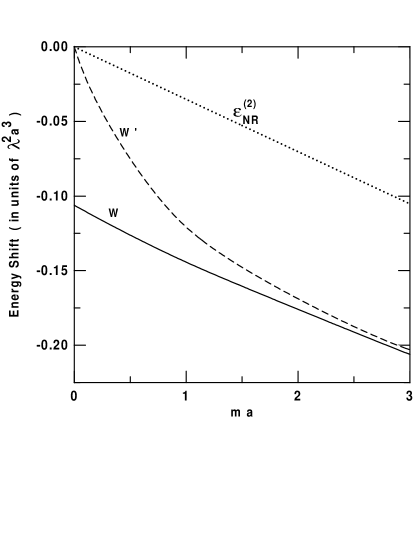
FIG. 3.: Relativistic energy shifts $W$ of method I (solid line), $W^{\prime}$ of method II (dashed line) and their nonrelativistic counterpart ${\epsilon_{\rm NR}}^{(2)}$ of Eq. (63) (dotted line) are shown in units of $\lambda^{2}a^{3}$ as functions of $ma$. The ${\epsilon_{\rm NR}}^{(2)}$ is not meaningful unless $ma\gg 1$.

IV The Dalgarno-Lewis method

The calculation of method II that was presented in Secs. II and III is somewhat involved. So it would be good to confirm it by repeating the calculation in a different manner. We do so by using the DL method. The DL method is an alternative form of perturbation theory in which summations over intermediate states are avoided [3, 4, 5]. As a price for it, one has to solve an inhomogeneous differential equation. The DL method is often used in calculating the electric polarizability of nonrelativistic bound systems. There is another similar, powerful method called logarithmic perturbation expansion [11, 12], which we do not use here. Consider any one of the energy levels. Let its unperturbed wave functions be $\psi^{(0)}(x)$ and its first order perturbation be $\psi^{(1)}(x)$. The $\psi^{(1)}(x)$ can be determined by the DL equation

$$(H_{0}-\epsilon^{(0)})\psi^{(1)}(x)=-V(x)\psi^{(0)}(x)\,,$$ (50)

where $\epsilon^{(0)}$ is the unperturbed energy, i.e., $\epsilon$ of Sec. III. We write $\psi^{(1)}$ as

$$\psi^{(1)}(x)=\left(\begin{array}[]{c}u^{(1)}(x)\\ v^{(1)}(x)\end{array}\right).$$ (53)

Its components are again subject to boundary condition (18),

$$v^{(1)}(a)=-u^{(1)}(a)\,.$$ (54)

When $\psi^{(1)}$ is found, the second order energy shift $\epsilon^{(2)}$ can be calculated by

$$\epsilon^{(2)}=\int^{\infty}_{-\infty}V(x)\psi^{{\dagger}(1)}(x)\psi^{(0)}(x)dx\,.$$ (55)

The summation over intermediate states is done implicitly. It is understood that there is no restriction on intermediate states due to the Pauli principle. Since it includes all intermediate states of negative as well as positive energies, $\epsilon^{(2)}$ is nothing but $W^{\prime}_{1}$ or $W^{\prime}_{-j}$ of Sec. II. If we take the unperturbed wave function for $|1\rangle$ for $|\psi^{(0)}(x)$, for example, we obtain $W^{\prime}_{1}$. Obviously the DL method is not useful for method I.

By solving Eq. (50) we obtain

$$u^{(1)}(x)=\frac{\lambda N}{2k^{2}}\left[mx\cos kx+\eta\epsilon k(x^{2}-a^{2})\sin kx\right.$$ (56)

$$\left.-\frac{\eta mk}{2\epsilon}\left(\frac{1}{\epsilon+m}+2a\right)\sin kx\right]\,,$$ (57)

$$v^{(1)}(x)=\frac{\lambda mN}{2\epsilon k^{2}}\left\{\frac{\eta\epsilon}{\epsilon+m}kx\sin kx+\left[\frac{1}{2}-(\epsilon-m)a\right.\right.$$ (58)

$$\left.\left.+\frac{\epsilon^{2}(\epsilon-m)}{m}(x^{2}-a^{2})\right]\cos kx\right\},$$ (59)

where $\eta=1(-1)$ for even (odd) parity. The $\epsilon$ and $k$ are $\epsilon^{(0)}$ and $k^{(0)}$, respectively. With these $u^{(1)}$ and $v^{(1)}$ in Eq. (55) we arrive at

$$\epsilon^{(2)} = {\frac{\lambda^{2}m}{24k^{4}\epsilon a[2(\epsilon a)^{2}+ma]}}\$$ (60)

$$\times \left\{2(ka)^{2}(ma+3)[4(\epsilon a)^{2}-6ma-3]\right.$$ (62)

$$\left.-15(ma)^{2}(2ma+1)\right\}\,.$$

This applies to any of the energy levels with an appropriate choice of $k$ that is subject to Eq. (21). We have explicitly confirmed that $\epsilon^{(2)}$ agrees with $W^{\prime}_{1}$ or $W^{\prime}_{-j}$ of method II for each of the energy levels and hence the same $W^{\prime}$ as that of Sec. III. The $\epsilon^{(2)}$ vanishes if $m=0$. This is consistent with what we found in Sec. III.

In the non-relativistic limit of $m\to\infty$, Eq. (54) is reduced to

$${\epsilon_{\rm NR}}^{(2)}=\frac{\lambda^{2}m}{24k^{4}}\left[4(ka)^{2}-15\right]\,,\hskip 11.38092ptka=\frac{\pi}{2}\,.$$ (63)

The nonrelativistic value of $ka$ follows from Eq. (21) with the plus sign and $m\to\infty$. Equation (55) agrees with the result for an infinite square-well potential of non-relativistic quantum mechanics [13]. The ${\epsilon_{\rm NR}}^{(2)}$ is compared with its relativistic counterparts $W$ and $W^{\prime}$ in Fig. 3. Note that even when $m$ is as large as $m=3/a$ (or $m\approx 600$ MeV if $a=1$ fm), the relativistic energy shifts are about twice as large as their nonrelativistic counterpart.

V summary and discussions

For a system consisting of a particle bound in a given potential together with its vacuum background, we examined the second order energy shift caused by external perturbation $V$. We examined two formally equivalent methods of calculation, I and II. Method I takes account of the Pauli principle in intermediate states whenever it is applicable. In method II the Pauli principle is completely ignored. We showed that, if the energy shifts of all occupied levels are summed up in method II, the terms violating the Pauli principle formally cancel out. Thus the two methods appear equivalent. This illustrates Feynman’s prescription.

This equivalence, however, is not free from ambiguity. We calculated the energy shift explicitly for the one-dimensional bag model with external perturbation $V(x)=\lambda x$. As shown in Fig. 3, the two methods lead to different energy shifts. Thus Feynman’s prescription fails in this example. For method II, we did the calculation in two different manners, one by summing up over the intermediate states and the other by using the DL method. The same result were obtained by two calculations. In method II the energy shifts of the individual occupied levels are unambiguously obtained. When they are summed over all negative energy states, however, an alternate series emerges. The sum of the series depends on how the summation is done. This is essentially the source of the discrepancy between the two apparently equivalent methods. The alternating series is hidden such that, if one simply follows method II, one would not notice it.

Feynman’s prescription fails in the specific example that we have described. A question naturally arises here. Does similar difficulty arise in more general situations? We suspect that it may well do. Let us first point out that, although we assumed a specific form of external perturbation $V(x)=\lambda x$, Feynman’s prescription fails in the one-dimensional bag model irrespectively of the form of $V(x)$. Again for simplicity let us assume $m=0$. Then the matrix element of $V(x)$ are of the form of

$$\int^{a}_{-a}V(x)\sin[(k-k^{\prime})x]dx\;\;\;\;{\rm or}\;\;\;\;\int^{a}_{-a}V(x)\cos[(k-k^{\prime})x]dx\,.$$ (64)

No matter how large $k$ and $k^{\prime}$ become, the matrix element is of the same form as that of Eq. (38). This feature remains essentially the same when $m$ becomes nonzero. In this connection, recall what we said in the last paragraph of Sec. III.

Next let us consider the three-dimensional bag model, subject to a constant external electric field. The perturbation interaction can be taken as $\lambda z=\lambda r\cos\theta$. For states with large quantum numbers, the radial part of the wave function is similar to the one-dimensional wave function. This is so in the sense that at large distances the spherical Bessel functions involved are like the sine and cosine functions. For the angular part, the matrix element of $\cos\theta$ between two adjacent angular momentum states has a part that remains finite no matter how large the angular momenta become. Therefore, the alternating series involved in method II will remain. We are aware of a few calculations of the electric and magnetic polarizabilities of the nucleon by using the bag model [14, 15, 16]. Method I was used in these calculations and hence the problem with method II was not encountered.

We have assumed that the energy spectrum of the unperturbed system is discrete. The case of continuum spectrum can be handled by enclosing the system in a very large cavity. The unperturbed Hamiltonian $H_{0}$ in this case can be that of the bag model (with a large radius) plus some other interaction that produces states localized, say, around the origin. Let us consider such a model in one dimension. The perturbation of the form of $V(x)=\lambda x$, if taken literally, would not make much sense because it becomes very large as $x$ approaches the cavity radius. If one chooses $V(x)$ such that it remains reasonably small within the entire cavity, one can treat it by perturbation theory. Then the calculation will go in a way essential the same as we have done. Feynman’s prescription will probably fail again.

As far as we know the example that we have presented is the first counter-example against Feynman’s prescription that seems to have been taken for granted for many years. If we have to choose between methods I and II, we are inclined to take method I and abandon method II that is based on Feynman’s prescription. We think that, if we encounter ambiguity by disregarding the Pauli principle, we should remain faithful to the Pauli principle in every step of calculation. In view of the fact that Feynman’s prescription has been used extensively, its possible failure may have serious implications.

REFERENCES

- [1] R.P. Feynman, Phys. Rev. 76, 749 (1949), in particular p. 755.
- [2] H. Miyazawa, Progr. Theor. Phys. 6, 801 (1951); S.D. Drell and J.D. Walecka, Phys. Rev. 120, 1069 (1960); J. Osada and M. Takeda, Progr. Theor. Phys. 24, 755 (1960); I. Hamamoto and H. Miyazawa, Phys. Rev. 123, 1860 (1961); D. Kiang and Y. Nogami, Nuovo Cimento 51, 59 (1967); M. Baranger, in Nuclear Structure and Nuclear Reactions, Procs. of the International School of Physics “Enrico Fermi” (Academic Press, New York, 1969), pp. 511-614, in particular Section ; S. Raimes, Many-Electron Theory (North-Holland, Amsterdam, 1972), Chapter 7.
- [3] A. Dalgarno and J.T. Lewis, Proc. Roy. Soc. London 233, 70 (1955).
- [4] Actually Kotani calculated the electric polarizability of the nonrelativistic hydrogen atom by the DL method before Ref.[3]; M. Kotani, Quantum Mechanics I (in Japanese) (Iwanami, Tokyo, 1951), Chapter 4.
- [5] M.A. Maize and C.A. Burkholder, Am. J. Phys. 63, 244 (1995).
- [6] We can start with a negative energy bound state, e.g., . If we do so, however, we will meet unnecessary, nonessential complications in the context of quantum field theory.
- [7] M.A. Maize, S. Paulson, and A. D’Avanti, Am. J. Phys. 65, 888 (1997).
- [8] F.A.B. Coutinho, Y. Nogami, and L. Tomio, Am. J. Phys. Submitted.
- [9] A. Chodos, R. Jaffe, K. Johnson, C. Thorn and V. Weisskopf, Phys. Rev. D 9, 3471 (1974).
- [10] F. Close, An Introduction to Quarks and Partons (Academic Press, New York, 1979).
- [11] Y. Aharonov and C.K. Au, Phys. Rev. Lett. 42, 1582 (1979); C.K. Au and Y. Aharonov, Phys. Rev. A 20, 2245 (1979).
- [12] F.A.B. Coutinho, Y. Nogami and F.M. Toyama, Am. J. Phys. 65, 788 (1997), and earlier references quoted there.
- [13] H.A. Marvromatis, Am. J. Phys. 59, 738 (1991).
- [14] P.C. Hecking and G.F. Bertsch, Phys. Lett. 99 B, 237 (1981).
- [15] A. Schäfer, B. Müller, D. Vasak and W. Greiner, Phys. Lett. 143 B, 323 (1984).
- [16] R. Weiner and W. Weise, Phys. Lett. B 159, 85 (1985).
Appendix
Let us first examine how of Eq. (47) and of Eq. (48) vanish. First note that