Accessible information and optimal strategies
for real symmetrical quantum sources

Abstract

We study the problem of optimizing the Shannon mutual information for sources of real quantum states i.e. sources for which there is a basis in which all the states have only real components. We consider in detail the sources ${\cal E}_{M}$ of $M$ equiprobable qubit states lying symmetrically around the great circle of real states on the Bloch sphere and give a variety of explicit optimal strategies. We also consider general real group-covariant sources for which the group acts irreducibly on the subset of all real states and prove the existence of a real group-covariant optimal strategy, extending a theorem of Davies (E. B. Davies, IEEE. Inf. Theory IT-24, 596 (1978)). Finally we propose an optical scheme to implement our optimal strategies, simple enough to be realized with present technology.

I Introduction

There are two principal measures of quality in the quantum detection problem for a given finite number of quantum states with fixed prior probabilities. One is the minimization of a specified Bayes cost, and the other is the maximization of the Shannon mutual information [1, 2, 3]. The former is useful if one has to reach a decision after performing a single quantum measurement whereas the latter is more relevant for the problem of transmitting as much classical information as possible using the given ensemble of states. In this paper we will consider the problem of maximizing the Shannon mutual information for a certain class of quantum ensembles.

In a general communication setting, let $\{x_{i}\in X\}$ be input letters and let $\{\xi_{i}\}$ be their prior probabilities. Let us denote output letters by $\{y_{j}\in Y\}$. Both the Bayes cost and the Shannon mutual information are defined in terms of the conditional probability $P(j|i)$ of obtaining output $y_{j}$ provided that the letter sent was $x_{i}$. The former is defined as

$$B(X:Y)=\sum_{ij}C_{ij}\xi_{i}P(j|i),$$ (1)

for a Bayes cost matrix $[C_{ij}]$, while the latter is defined as

$$I(X:Y)=\sum_{i}\xi_{i}\sum_{j}P(j|i)\log\frac{P(j|i)}{\displaystyle\sum_{k}\xi_{k}P(j|k)}.$$ (2)

(Since all the results in this paper are valid for any logarithm base, we shall specify the base only where necessary.) In classical information theory, the channel matrix $[P(j|i)]$ is given and fixed, characterising the noise in the channel. In contrast, in a quantum information theoretic context where signal carriers are to be quantum states transmitted without noise, the channel matrix generally becomes a variable. This is because the act of quantum detection itself generally has a probabilistic output so the channel matrix is dependent on the choice of quantum detection strategy. More precisely, the input letters correspond to a set of positive trace class operators of trace one $\{\hat{\rho}_{i}\}$ on a Hilbert space ${\cal H}_{s}$. A quantum detection strategy is described by a positive operator-valued measure (POVM) on ${\cal H}_{s}$. A POVM is any set $\{\hat{\pi}_{j}\}$ of hermitian positive operators forming a resolution of the identity:

$$\hat{\pi}_{j}^{\dagger}=\hat{\pi}_{j},\quad\hat{\pi}_{j}\geq 0\quad\forall j,\quad\sum_{j}\hat{\pi}_{j}=\hat{I}.$$ (3)

The detection operator $\hat{\pi}_{j}$ corresponds to the output letter $y_{j}$ and the conditional probabilities are given by

$\displaystyle P(j|i)={\rm Tr}(\hat{\pi}_{j}\hat{\rho}_{i}).$Thus in the quantum context the optimization of $I(X:Y)$ is carried out with respect to the choice of POVM $\{\hat{\pi}_{j}\}$ for fixed ensemble ${\cal E}=\{\hat{\rho}_{i};\xi_{i}\}$ (i.e. with fixed letter states $\hat{\rho}_{i}$ and fixed prior probabilities $\xi_{i}$). The maximum value of $I(X:Y)$ is called the accessible information of the ensemble $\cal E$.

The set $\cal P$ of all POVM’s is a convex set and $I(X:Y)$ enjoys the following fundamental property:
(CONV): For a fixed ensemble ${\cal E}=\{\hat{\rho}_{i};\xi_{i}\}$, $I(X:Y)$ is a convex function on $\cal P$.
A proof of (CONV) is given in theorem 2.7.4 of [4]. Let $I({\cal E}:{\cal A})$ denote the mutual information obtained from the POVM $\cal A$ applied to the ensemble $\cal E$. Then if $\cal A$ is a convex combination of POVMs ${\cal A}_{i}$:

$\displaystyle{\cal A}=p_{1}{\cal A}_{1}+\cdots p_{n}{\cal A}_{n}.$it follows from (CONV) that

$$I({\cal E}:{\cal A})\leq\sum_{i}p_{i}I({\cal E}:{\cal A}_{i})\leq\max_{i}I({\cal E}:{\cal A}_{i}).$$ (4)

The Bayes cost $B(X:Y)$ is an affine concave function on the convex set $\cal P$. Therefore the Bayes cost minimization problem is a kind of linear programming problem and is expected to have a unique solution. A necessary and sufficient condition for specifying the optimum solution is known[1, 2]. On the other hand, the Shannon mutual information $I(X:Y)$ is a nonlinear and convex function on $\cal P$. The maximization of this quantity is a much harder problem and only a necessary condition for the optimum is known [1]. Thus the maximization of $I(X:Y)$ with respect to the detection strategy $\{\hat{\pi}_{j}\}$ is a basic and open problem in quantum information theory.

In this problem, the number of outputs is not necessarily the same as the number of the inputs. The optimum solution is not necessarily unique either. However it is known that there must be at least one optimum solution which corresponds to an extreme point of the convex set $\cal P$. This is due to the convexity of the function $I(X:Y)$. Such an extreme point is a set of rank one elements, which means that each $\hat{\pi}_{j}$ has the form $\kappa\left|v\right\rangle\left\langle v\right|$ where $\left|v\right\rangle$ is a pure state and $0\leq\kappa\leq 1$. The number of elements, $N$, can be bounded by $d\leq N\leq d^{2}$ where $d$ is the dimension of the Hilbert space ${\cal H}_{s}$ of which the input state ensemble $\{\hat{\rho}_{i}\}$ is made [5]. $I(X:Y)$ is also possibly maximized at some interior points of $\cal P$ as well. In that case the number of outcomes may exceed $d^{2}$. Explicit examples of optimal solutions have been given for binary ensembles [6, 7, 8] and for the ensemble of four qubit states with tetrahedral symmetry [5]. The latter is a specific example of a general result of Davies [5] characterising the form of an optimal strategy for any symmetrical ensemble whose symmetry group acts irreducibly on the whole state space.

In this paper we will study the accessible information and corresponding optimal strategies for an ensemble ${\cal E}_{M}$ of $M$ qubit states with symmetry group $\mbox{Z}_{M}$, the group of integers modulo $M$. Some of our results will also apply to more general ensembles. ${\cal E}_{M}$ may be explicitly described as follows. Let $\{\left(\begin{array}[]{c}1\\ 0\end{array}\right),\left(\begin{array}[]{c}0\\ 1\end{array}\right)\}$ be the $z$-spin eigenstates and write $\left|\psi_{0}\right\rangle=\left(\begin{array}[]{c}1\\ 0\end{array}\right)$. Let

$$\hat{V}\equiv{\rm exp}(-i{\pi\over M}\hat{\sigma}_{y})=\left(\begin{array}[]{cc}\cos{{\pi}\over M}&-\sin{{\pi}\over M}\\ \sin{{\pi}\over M}&\cos{{\pi}\over M}\end{array}\right).$$ (5)

Then ${\cal E}_{M}$ consists of the $M$ states

$$\left|\psi_{k}\right\rangle=\hat{V}^{k}\left|\psi_{0}\right\rangle=\left(\begin{array}[]{c}\cos\frac{k\pi}{M}\\ \sin\frac{k\pi}{M}\end{array}\right),\quad k=0,\ldots,M-1,$$ (6)

taken with equal prior probabilities $\xi_{k}=\frac{1}{M}$. Note that these states (in the $z$-spin basis) involve only real components. On the Bloch sphere they are equally spaced around a great circle $C$ in the $x-z$ plane consisting of all real states. The antipodal points which have $C$ as equator, are the two $\hat{\sigma}_{y}$ eigenstates. Thus ${\cal E}_{M}$ is clearly symmetrical with respect to the group $\mbox{Z}_{M}$ whose generator is represented by ${2\pi\over M}$ rotation about the axis joining the $\hat{\sigma}_{y}$ eigenstates. At the Hilbert space level the operators $\hat{V}^{k}$ in Eq. (5) provide a projective unitary representation of $\mbox{Z}_{M}$ (e.g. $\hat{V}^{M}=-I$ and c.f. Eq. (7) later).

This symmetry group does not act irreducibly on the whole state space. Indeed the $\hat{\sigma}_{y}$ eigenstates are left invariant by the group action. (Irreducibility on the whole state space requires that the only invariant point is the maximally mixed state ${1\over 2}\hat{I}$.) Hence we cannot apply Davies’ theorem [5] to provide an optimal strategy for ${\cal E}_{M}$. Nevertheless we will prove that the conclusion of Davies’ theorem remains true in this case i.e. that there exists a pure state $\left|a_{0}\right\rangle$ such that the $\mbox{Z}_{M}$-symmetric POVM

$\displaystyle{\cal A}_{M}=\{{2\over M}\left|a_{k}\right\rangle\left\langle a_{k}\right|:k=0,\ldots,M-1\}\quad\mbox{where $\left|a_{k}\right\rangle=\hat{V}^{k}\left|a_{0}\right\rangle$},$is an optimal strategy for ${\cal E}{{}_{M}}$. Furthermore we will show that $\left|a_{0}\right\rangle$ may be taken to be the state orthogonal to $\left|\psi_{0}\right\rangle$.

The case $M=3$ is of particular interest. It is the so-called trine ensemble which has been much studied [9, 10, 11]. Holevo in 1973 [9] showed that no von Neumann measurement in ${\cal H}_{2}$ can be an optimal strategy, demonstrating the necessity of considering more general POVMs in quantum detection theory. Since that time it has been conjectured that the strategy ${\cal A}_{3}$ above is optimal for the trine source. Our results resolve this conjecture affirmatively.

The strategy ${\cal A}_{M}$ has $M$ elements. However, as noted above, for ensembles in $d=2$ dimensions there is always an optimal strategy with at most $d^{2}=4$ elements (which does not increase with $M$). We will show that the ensembles ${\cal E}_{M}$ always have an optimal strategy with at most 3 elements and explicit strategies of this form will be described for all $M$. If $M$ is even then ${\cal E}_{M}$ consists of ${M\over 2}$ pairs of orthogonal states. Let $\{\left|\xi\right\rangle,\left|\eta\right\rangle\}$ be any one of these pairs. We will show that the two-element POVM $\{\left|\xi\right\rangle\left\langle\xi\right|,\left|\eta\right\rangle\left\langle\eta\right|\}$ (a regular von Neumann measurement) is always an optimal strategy when $M$ is even. We will also describe further optimal $K$-element POVMs where $K$ lies between 3 and $M$.

II A Group-theoretic Approach

We begin by setting up a group-theoretic formalism for symmetric ensembles, leading to a main result (theorem 1) which applies to symmetric ensembles of real states in any dimension $d\geq 2$. An essential requirement in many of our results will be that various states and unitary operators be real. The requirement that a state or operator be real has of course, no intrinsic physical meaning. When we speak of real states and real operators we will always mean simply that there exists a basis of the Hilbert space relative to which all the required objects simultaneously have real components or real matrix elements.

A projective unitary representation of a group $G$ is an assignment of a unitary operation $\hat{U}_{g}$ to each member of $G$ satisfying

$$\hat{U}_{g_{1}}\hat{U}_{g_{2}}=e^{i\phi(g_{1},g_{2})}\hat{U}_{g_{1}g_{2}},$$ (7)

where the phases $\phi(g_{1},g_{2})$ may be chosen arbitrarily. A finite ensemble ${\cal E}$ of equiprobable (generally mixed) states is said to be symmetric with respect to the group $G$, or $G$-covariant, if the following condition is satisfied: there is a projective unitary representation $\{\hat{U}_{g}\}$ of $G$ such that for all $g$, $\hat{U}_{g}\hat{\rho}\hat{U}_{g}^{\dagger}$ is in $\cal E$ whenever $\hat{\rho}$ is in $\cal E$. We write

$$g\hat{\rho}=\hat{U}_{g}\hat{\rho}\hat{U}_{g}^{\dagger},$$ (8)

for the action of $g$ on the state $\hat{\rho}$. The phases $\phi(g_{1},g_{2})$ do not appear in Eq. (8) and $g_{1}(g_{2}(\hat{\rho}))=(g_{1}g_{2})(\hat{\rho})$. Note that, in contrast to Davies [5] we do not require that $G$ parameterises $\cal E$ i.e. $G$ need not act transitively on the set of states of $\cal E$. For example, ${\cal E}_{M}$ is $\mbox{Z}_{M}$-covariant and the action is transitive, but ${\cal E}_{2N}$ is also $\mbox{Z}_{2}$- and $\mbox{Z}_{N}$-covariant via non-transitive actions.

A $G$-covariant POVM $\cal A$ (for the projective unitary representation $\{\hat{U}_{g}\}$) is a POVM such that $\hat{U}_{g}\hat{A}\hat{U}_{g}^{\dagger}$ is in $\cal A$ whenever $\hat{A}$ is in $\cal A$. We write

$$g\hat{A}\equiv\hat{U}_{g}\hat{A}\hat{U}_{g}^{\dagger},$$ (9)

for the action of $g$ on a POVM element $\hat{A}$. From Eqs. (8) and (9) we see that ${\rm\,Tr}\,(\hat{A}\hat{\rho})={\rm\,Tr}\,(g\hat{A}\cdot g\hat{\rho})$ i.e. the probability of outcome $\hat{A}$ on state $\hat{\rho}$ is $G$-invariant. Hence

$${\rm\,Tr}\,(g\hat{A}\cdot\hat{\rho})={\rm\,Tr}\,(\hat{A}\cdot g^{-1}\hat{\rho}),$$ (10)

so that the set of probabilities of the $G$-shifted outputs $g\hat{A}$ on a fixed input $\hat{\rho}$ are obtained as a permutation of the set of probabilities of the unshifted output $\hat{A}$ acting on suitably shifted inputs.

Let $\cal E$ be a $G$-covariant ensemble with projective unitary representation $\{\hat{U}_{g}\}$. We aim to find conditions on $\{\hat{U}_{g}\}$ which will guarantee the existence of a $G$-covariant POVM ${\cal A}=\{\hat{A}_{g}:g\in G\}$ with elements parameterised by $G$, and having group action $g\hat{A}_{h}=\hat{A}_{gh}$. Thus if $e$ is the identity of $G$ we have

$$\hat{A}_{g}=\hat{U}_{g}\hat{A}_{e}\hat{U}_{g}^{\dagger},$$ (11)

and we require

$$\hat{M}\equiv\sum_{g\in G}\hat{A}_{g}=\hat{I}.$$ (12)

(Later we will take the elements of $\cal A$ to be rank 1 and consider the question of when $\cal A$ is an optimal strategy for $\cal E$.) From Eq. (11) we see that $\hat{M}$ commutes with all the $\hat{U}_{g}$’s:

$$\hat{U}_{g}\hat{M}=\hat{M}\hat{U}_{g}.$$ (13)

Thus if the set $\{\hat{U}_{g}\}$ acts irreducibly on the state space (i.e. there is no proper invariant subspace) the Schur’s lemma will guarantee that Eq. (12) holds. This fact is used by Davies [5] to characterise an optimal strategy for any $G$-covariant ensemble whose symmetry group acts irreducibly on the whole state space. However this condition of full irreducibility on the whole state space is not necessary for Eq. (12) to hold. We will use the following more general form of Schur’s lemma:

Lemma 1: Let $\{\hat{M}_{g}\}$ be any set of non-singular $d$ by $d$ matrices over some field $F$ which acts irreducibly on the vector space $V=F^{d}$ (i.e. there is no proper subspace mapped to itself by all the $\hat{M}_{g}$’s). Suppose that $\hat{K}$ is any matrix that commutes with all the $\hat{M}_{g}$’s:

$$\hat{K}\hat{M}_{g}=\hat{M}_{g}\hat{K}.$$ (14)

Then:
(a) either $\hat{K}=0$ or $\hat{K}$ is non-singular,
(b) If $\hat{K}$ has a non-zero eigenvalue $\lambda$ in $F$, then $\hat{K}=\lambda\hat{I}$.

Proof: (a) Let $\hat{K}(V)$ denote the image of $V$ under the map $\hat{K}$ and similarly for $\hat{M}_{g}(V)$. Since $\hat{M}_{g}$ is non-singular we have $\hat{M}_{g}(V)=V$. By Eq. (14) we have $\hat{M}_{g}\hat{K}(V)=\hat{K}\hat{M}_{g}(V)=\hat{K}(V)$ i.e. $\hat{K}(V)$ is an invariant subspace. Hence either $\hat{K}(V)=0$ (in which case $\hat{K}=0$) or else $\hat{K}(V)=V$ (in which case $\hat{K}$ is non-singular).
(b) If $\hat{K}$ has eigenvalue $\lambda$ in $F$ then $\hat{B}=\hat{K}-\lambda\hat{I}$ is singular. Also $\hat{B}\hat{M}_{g}=\hat{M}_{g}\hat{B}$ for all $g$. Hence by (a), $\hat{B}$ must be zero i.e. $\hat{K}=\lambda\hat{I}$.  

We will apply this lemma with $F=\mbox{I$\!$R}$ to obtain useful results about $G$-covariant ensembles of real states whose group $G$ acts irreducibly only on the restricted set $\mbox{I$\!$R}^{d}$ of real states (but not necessarily irreducibly on the full state space). This is the case for our ensembles ${\cal E}_{M}$. Let $|G|$ denote the size of $G$ and let $d={\rm\,Tr}\,\hat{I}$ be the dimension of the Hilbert space.

Lemma 2: Suppose that $\{\hat{U}_{g}\}$ is a projective unitary representation of $G$ such that $\hat{U}_{g}$ are all real matrices and $\{\hat{U}_{g}\}$ acts irreducibly on $\mbox{I$\!$R}^{d}$. Let $\left|v\right\rangle\in\mbox{I$\!$R}^{d}$ be any real state. Write

$\displaystyle\hat{A}_{g}={d\over|G|}\hat{U}_{g}\left|v\right\rangle\left\langle v\right|\hat{U}_{g}^{\dagger}.$Then $\{\hat{A}_{g}:g\in G\}$ is a $G$-covariant POVM i.e. $\sum_{g\in G}\hat{A}_{g}=\hat{I}$.

Proof: Let $\hat{M}=\sum_{g\in G}\hat{A}_{g}$. Then $\hat{M}$ is a real matrix and $\hat{M}\hat{U}_{g}=\hat{U}_{g}\hat{M}$ for all $g\in G$. Also $\hat{M}$ is a hermitian positive matrix (being a sum of projectors with positive coefficients) so it has a real positive eigenvalue $\lambda>0$. By the previous lemma, $\hat{M}=\lambda\hat{I}$. Since ${\rm\,Tr}\,\hat{A}_{g}={d\over|G|}$ for all $g$, we get ${\rm\,Tr}\,\hat{M}=d={\rm\,Tr}\,\hat{I}$ so $\lambda=1$.  

Theorem 1: Let $\cal E$ be any ensemble of equiprobable real states in dimension $d$. Suppose that $\cal E$ is $G$-covariant with respect to a projective unitary representation $\{\hat{U}_{g}\}$ of real matrices which acts irreducibly on $\mbox{I$\!$R}^{d}$. Then there exists a real pure state $\left|v\right\rangle$ such that the $G$-covariant POVM ${\cal D}=\{\hat{D}_{g}:g\in G\}$ defined by

$\displaystyle\hat{D}_{g}={d\over|G|}\hat{U}_{g}\left|v\right\rangle\left\langle v\right|\hat{U}_{g}^{\dagger},$is an optimal strategy for $\cal E$.

Proof: We will work in the basis with respect to which the states of $\cal E$ and the matrices $\hat{U}_{g}$ have real entries. Let ${\cal A}=\{\hat{A}_{1},\ldots,\hat{A}_{n}\}$ be any optimal POVM for $\cal E$. We will transmogrify $\cal A$ into the required form while preserving optimality. First strip off all imaginary parts of the entries of the matrices $\hat{A}_{k}$. Let $\tilde{A}_{k}=Re(\hat{A}_{k})$ and $\tilde{\cal A}=\{\tilde{A}_{1},\ldots,\tilde{A}_{n}\}$. Then $\tilde{\cal A}$ is again a POVM and has real symmetric matrices as elements. (To see that $\tilde{A}_{k}$ is a positive matrix note that $A_{k}$ positive implies that the complex conjugate $\hat{A}^{*}_{k}$ is positive so $\tilde{A}_{k}={1\over 2}(\hat{A}_{k}+\hat{A}^{*}_{k})$ must be positive. Also $\sum\hat{A}_{k}=\hat{I}$ and $\hat{I}$ is real so $\sum\tilde{A}_{k}=I$ too.) Next note that ${\rm\,Tr}\,\hat{A}_{k}\hat{\rho}={\rm\,Tr}\,\tilde{A}_{k}\hat{\rho}$ for any real state $\hat{\rho}$ (since $Im(\hat{A}_{k})$ is antisymmetric) so $\tilde{\cal A}$ remains an optimal strategy.

In general $\tilde{\cal A}$ will not have rank 1 elements even if $\cal A$ had rank 1 elements. Thus decompose each $\tilde{A}_{k}$ into its rank 1 eigenprojectors (multiplied by the corresponding eigenvalues) which are necessarily real as the eigenvalues/vectors of any real symmetric matrix are real. Then form the larger POVM ${\cal B}=\{\hat{B}_{1},\ldots,\hat{B}_{m}\}$ comprising all the scaled rank 1 eigenprojectors above. Such a refinement of a POVM can never decrease the mutual information so $\cal B$ with real rank 1 elements, is still optimal.

Now look at

$$\hat{C}_{kg}={1\over|G|}g\hat{B}_{k}\quad\mbox{for $g\in G$ and $k=1,\ldots,m$}.$$ (15)

Note that $\sum_{kg}\hat{C}_{kg}=\hat{I}$ since $\sum\hat{B}_{k}=\hat{I}$ and $g\hat{I}=\hat{I}$ for all $g$. Let ${\cal C}=\{\hat{C}_{kg}\}$ be the corresponding POVM with $|G|m$ elements. Thus $\cal C$ is $G$-covariant but the action of $G$ is not transitive. We finally aim to cut down $\cal C$ to a smaller optimal $G$-covariant POVM with elements labeled by $G$.

Let $I({\cal E}:{\cal A})$ denote the mutual information obtained from any POVM $\cal A$ applied to any ensemble $\cal E$. First we show that $I({\cal E}:{\cal C})=I({\cal E}:{\cal B})$ so that $\cal C$ remains optimal. Let us label the inputs by $i\in{\cal I}$ and denote conditional probabilities for $\cal C$ by $P(kg|i)$. Denote the conditional probabilities for $\cal B$ by $P_{B}(k|i)$ and let $\xi$ be the constant prior input probability. Then

$\displaystyle P(kg|i)={\rm\,Tr}\,\hat{C}_{kg}\hat{\rho}_{i}={1\over|G|}{\rm\,Tr}\,g\hat{B}_{k}\cdot\hat{\rho}_{i}.$According to Eq. (10), for each fixed $g$ and $k$ the resulting set of probabilities labelled by $i\in{\cal I}$, will be just a permutation of the set $P_{B}(k|i)$, rescaled by ${1\over|G|}$. Thus

$\displaystyle\sum_{l}\xi P(kg|l)={1\over|G|}\sum_{l}\xi P_{B}(k|l),$will be independent of $g$ and also

$\displaystyle\sum_{i}P(kg|i)\log{P(kg|i)\over\xi\sum_{l}P(kg|l)}={1\over|G|}\sum_{i}P_{B}(k|i)\log{P_{B}(k|i)\over\sum_{l}\xi P_{B}(k|l)},$will be independent of $g$. The mutual informations $I({\cal E}:{\cal C})$ and $I({\cal E}:{\cal B})$ are given by (c.f. Eq. (2)):

$\displaystyle I({\cal E}:{\cal C})=\sum_{i}\xi\sum_{kg}P(kg|i)\log{P(kg|i)\over\xi\sum_{l}P(kg|l)},$

$\displaystyle I({\cal E}:{\cal B})=\sum_{i}\xi\sum_{k}P_{B}(k|i)\log{P_{B}(k|i)\over\xi\sum_{l}P_{B}(k|l)}.$On substituting the above $G$-invariant expressions into $I({\cal E}:{\cal C})$ we readily get $I({\cal E}:{\cal C})=I({\cal E}:{\cal B})$. (Our argument is actually an explicit example of the claim in lemma 5 of [5]). Hence $\cal C$ remains optimal.

Finally note that for each $i$, $\hat{B}_{i}/({\rm\,Tr}\,\hat{B}_{i})$ is a real pure state so by lemma 2,

$\displaystyle{\cal D}_{i}=\left\{{d\over|G|}{g\hat{B}_{i}\over{\rm\,Tr}\,\hat{B}_{i}}:g\in G\right\},$is a POVM for each $i$. Now ${{\rm\,Tr}\,\hat{B}_{i}\over d}{\cal D}_{i}=\{{1\over|G|}g\hat{B}_{i}:g\in G\}$ so $\cal C$ is a convex combination

$\displaystyle{\cal C}=\sum_{i=1}^{m}{{\rm\,Tr}\,\hat{B}_{i}\over d}{\cal D}_{i}.$Hence by Eq. (4)

$\displaystyle I({\cal E}:{\cal C})\leq\max_{i}I({\cal E}:{\cal D}_{i}).$Since $\cal C$ was optimal it follows that at least one of the ${\cal D}_{i}$’s is optimal. This gives an optimal $G$-covariant POVM with real rank 1 elements, parameterised by $G$, completing the proof.  

III Optimal Strategies for ${\cal E}_{M}$

We now return to the $\mbox{Z}_{M}$-covariant ensemble ${\cal E}_{M}$ in 2 dimensions, comprising the states

$\displaystyle\left|\psi_{k}\right\rangle=\left(\begin{array}[]{c}\cos{k\pi\over M}\\ \sin{k\pi\over M}\end{array}\right),\quad k=0,\ldots,M-1,$with equal prior probabilities ${1\over M}$. According to theorem 1, there must exist an optimal $\mbox{Z}_{M}$-covariant POVM ${\cal A}=\{\hat{A}_{0},\ldots,\hat{A}_{M-1}\}$ with $M$ real rank 1 elements. The elements will have the form $\hat{A}_{j}=\left|a_{j}\right\rangle\left\langle a_{j}\right|$ with

$$\left|a_{j}\right\rangle=\hat{V}^{j}\left|a_{0}\right\rangle=\sqrt{2\over M}\left(\begin{array}[]{c}\cos(\theta+{j\pi\over M})\\ \sin(\theta+{j\pi\over M})\end{array}\right),\quad j=0,\ldots,M-1,$$ (16)

and $\hat{V}$ is given in Eq. (5). The conditional probabilities $p(j|k)=|\left\langle a_{j}|\psi_{k}\right\rangle|^{2}$ may be readily computed and after some rearrangement we obtain the mutual information $I(\theta)$ explicitly as

$$I(\theta)={1\over M}\sum_{k=0}^{M-1}(1+\cos(2\theta-{2k\pi\over M}))\log(1+\cos(2\theta-{2k\pi\over M})).$$ (17)

In this section, the base of the logarithm is taken as $e$. (For this base the numerical value of Eq. (17) is the amount of information in nats rather than bits.) From the symmetry, $I(\theta)$ is a periodic function with period $\pi\over M$. Figure 1 shows numerical plots of $I(\theta)$ for $M=2,3,4$ and 5 and illustrates the following basic property:

Lemma 3: For each $M$, $I(\theta)$ has a global maximum at $\theta={\pi\over 2}$.

Proof: Since $|\cos(2\theta-{{2k\pi}\over M})|<1$, $I(\theta)$ can be expanded by using the formula

$$(1+x)\ln(1+x)=x+\sum_{n=2}^{\infty}{{(-1)^{n}}\over{n(n-1)}}x^{n},\quad|x|<1,$$ (18)

We get

$$I(\theta) = {1\over M}\sum_{k=0}^{M-1}\Big{[}{\rm cos}(2\theta-{{2k\pi}\over M})+\sum_{n=2}^{\infty}{{(-1)^{n}}\over{n(n-1)}}{\rm cos}^{n}(2\theta-{{2k\pi}\over M})\Big{]}$$ (19)

$$= {1\over M}\sum_{n=2}^{\infty}{{(-1)^{n}}\over{n(n-1)}}\sum_{k=0}^{M-1}{\rm cos}^{n}(2\theta-{{2k\pi}\over M}).$$ (20)

since $\sum_{k=0}^{M-1}{\rm cos}(2\theta-{{2k\pi}\over M})=0$. Next we separate out the even and odd parts of the series and replace powers of cosines by multiple angle cosines to get:

$$I(\theta) = {1\over M}\sum_{n=1}^{\infty}{{(-1)^{2n}}\over{2n(2n-1)}}\sum_{k=0}^{M-1}{\rm cos}^{2n}(2\theta-{{2k\pi}\over M})$$ (21)

$$+ {1\over M}\sum_{n=1}^{\infty}{{(-1)^{2n+1}}\over{(2n+1)2n}}\sum_{k=0}^{M-1}{\rm cos}^{2n+1}(2\theta-{{2k\pi}\over M})$$ (22)

$$= {1\over M}\sum_{n=1}^{\infty}{{(-1)^{2n}}\over{2n(2n-1)}}\sum_{k=0}^{M-1}{1\over{2^{2n-1}}}\Big{\{}{1\over 2}\left(\begin{array}[]{c}2n\cr n\end{array}\right)+\sum_{l=0}^{n-1}\left(\begin{array}[]{c}2n\cr l\end{array}\right){\rm cos}\left[(2n-2l)(2\theta-{{2k\pi}\over M})\right]\Big{\}}$$ (27)

$$+ {1\over M}\sum_{n=1}^{\infty}{{(-1)^{2n+1}}\over{(2n+1)2n}}\sum_{k=0}^{M-1}{1\over{2^{2n}}}\Big{\{}\sum_{l=0}^{n}\left(\begin{array}[]{c}2n+1\cr l\end{array}\right){\rm cos}\left[(2n+1-2l)(2\theta-{{2k\pi}\over M})\right]\Big{\}},$$ (30)

Then recall that

$$\sum_{k=0}^{M-1}{\rm cos}\left(L{{2k\pi}\over M}\right)=\left\{\begin{array}[]{rl}M&\quad\mbox{for }{L/M}=q\mbox{ (integer)}\\ 0&\quad\mbox{for }{L/M}\neq\mbox{ integer}\end{array}\right..$$ (31)

Applying this to Eq. (30) with $L=2n-2l$ and $L=2n+1-2l$ in the even and odd series, we get:

$$I(\theta) = \sum_{n=1}^{\infty}{{(-1)^{2n}}\over{2n(2n-1)2^{2n-1}}}\Big{[}{1\over 2}\left(\begin{array}[]{c}2n\cr n\end{array}\right)+\sum_{l=0}^{n-1}\sum_{q=0}^{\infty}\left(\begin{array}[]{c}2n\cr l\end{array}\right){\rm cos}(2\theta qM)\delta_{2n-2l,qM}\Big{]}$$ (36)

$$+ \sum_{n=1}^{\infty}{{(-1)^{2n+1}}\over{(2n+1)2n2^{2n}}}\Big{[}\sum_{l=0}^{n}\sum_{q=0}^{\infty}\left(\begin{array}[]{c}2n+1\cr l\end{array}\right){\rm cos}(2\theta qM)\delta_{2n+1-2l,qM}\Big{]}$$ (39)

$$= \sum_{n=1}^{\infty}{1\over{2n(2n-1)2^{2n}}}\left(\begin{array}[]{c}2n\cr n\end{array}\right)+\sum_{q=0}^{\infty}f(qM)(-1)^{qM}{\rm cos}(2\theta qM),$$ (42)

where

$$f(qM)=\sum_{n=1}^{\infty}\sum_{l=0}^{n-1}{{\left(\begin{array}[]{c}2l+qM\cr l\end{array}\right)}\over{(2l+qM)(2l+qM-1)2^{2l+qM-1}}}\left(\delta_{2n-2l,qM}+\delta_{2n+1-2l,qM}\right).$$ (43)

Since $f(qM)>0$, $I(\theta)$ is maximized when $(-1)^{qM}{\rm cos}(2\theta qM)=1$, that is, $\theta={\pi\over 2}$ for all $M$.  

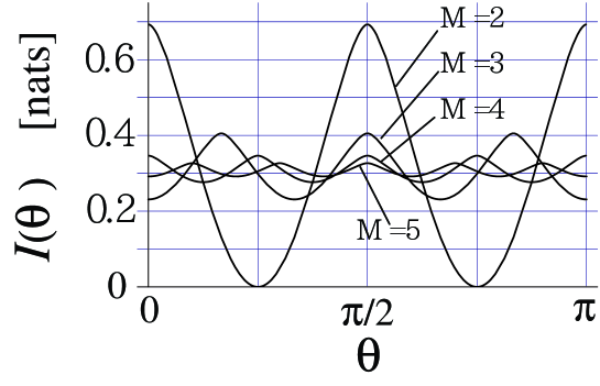
FIG. 1.: The Shannon mutual information $I(\theta)$ in nats versus the optimization parameter $\theta$ for $M=$2, 3, 4 and 5.

Hence in general an optimal strategy for ${\cal E}_{M}$ consists of choosing a real rank 1 POVM with elements $\hat{A}_{k}$ lying in directions orthogonal to the input states $\left|\psi_{k}\right\rangle$. This POVM will be denoted by ${\cal A}_{M}$. The output $\hat{A}_{k}$ signifies with certainty that the input was not $\left|\psi_{k}\right\rangle$ but leaves a residual uncertainty in the remaining signal states.

For a given ensemble $\cal E$ the optimal strategy is not unique and in practice it may be of interest to find optimal POVMs with the minimum number of elements. The $G$-covariant optimal POVM above has $M$ elements and we note here some ways of reducing this number using the group theoretic approach. In the next section, by different methods, we will show that 3 elements always suffice for any real qubit source, and develop corresponding strategies for the ${\cal E}_{M}$’s.

Lemma 4: Suppose that $k\neq 1$ divides $M$ exactly. Then there is a $\mbox{Z}_{k}$-covariant optimal POVM for ${\cal E}_{M}$ with $k$ real rank 1 elements.

Proof: Since $k$ divides $M$, $\mbox{Z}_{M}$ has a subgroup isomorphic to $\mbox{Z}_{k}$ and so ${\cal E}_{M}$ is $\mbox{Z}_{k}$-covariant. Since $k\neq 1$, the action of $\mbox{Z}_{k}$ contains a non-trivial rotation so it acts irreducibly on $\mbox{I$\!$R}^{2}$. Thus theorem 1 immediately gives the required result. 

Remark: Lemma 4 may also be obtained by a convexity argument as follows. We will illustrate the idea with the specific example of $M=15$ and $k=3$. The general case is a straightforward generalisation. $\mbox{Z}_{15}=\{0,1,\ldots,14\}$ has the subgroup $\{0,5,10\}$ isomorphic to $\mbox{Z}_{3}$. Let ${\cal A}_{15}=\{\hat{A}_{0},\hat{A}_{1},\ldots,\hat{A}_{14}\}$ be the optimal strategy given by theorem 1 and lemma 3, with the direction of $\hat{A}_{k}$ being orthogonal to the $k^{\rm th}$ state of ${\cal E}_{15}$. According to lemma 2, the three directions 0,5,10 corresponding to the subgroup, may be used to define a POVM. We just need to rescale $\hat{A}_{0},\hat{A}_{5}$ and $\hat{A}_{10}$ so that they add up to $\hat{I}$. The scaling factor is ${M\over k}=5$. Thus ${\cal B}_{0}=\{5\hat{A}_{0},5\hat{A}_{5},5\hat{A}_{10}\}$ is a POVM. Now $\hat{I}$ is always $G$ invariant so we can apply the group elements $l=1,2,3$ and 4 of $\mbox{Z}_{15}$ to ${\cal B}_{0}$ to obtain POVMs

$\displaystyle{\cal B}_{l}\equiv l{\cal B}_{0}=\{5\hat{A}_{l},5\hat{A}_{l+5},5\hat{A}_{l+10}\}\quad\mbox{for $l=0,1,2,3,4$}.$Note that the ${\cal B}_{l}$’s have elements parameterised by the cosets of $\mbox{Z}_{3}$ in $\mbox{Z}_{15}$. Also by symmetry of the construction, $I({\cal E}_{15}:{\cal B}_{l})$ is independent of $l$. Furthermore ${\cal A}_{15}$ is a uniform convex combination of the ${\cal B}_{l}$’s

$\displaystyle{\cal A}_{15}=\sum_{l=0}^{4}{1\over 5}{\cal B}_{l},$so by Eq. (4):

$\displaystyle I({\cal E}_{15}:{\cal A}_{15})\leq\max_{l}I({\cal E}_{15}:{\cal B}_{l}).$Since ${\cal A}_{15}$ was optimal we see that ${\cal B}_{l}$ is optimal for each $l$. This gives the result of lemma 4 and also identifies the directions of the $k$ element POVM as being any chosen symmetrical set of $k$ directions orthogonal to corresponding states of ${\cal E}_{M}$. 

An immediate special case is:

Corollary: If $M$ is even then ${\cal E}_{M}$ is made up of ${M\over 2}$ pairs of orthogonal states. The von Neumann measurement defined by any one of these orthogonal pairs is an optimal strategy for ${\cal E}_{M}$. 

Thus if $M$ is composite we can significantly reduce the number of elements in our optimal strategy but if $M$ is prime then this number remains large. In the next section we give a different approach to reducing the number of elements, showing that just 3 elements always suffices for any ensemble of real qubit states.

IV Optimal POVMs with 3 Elements

Davies [5] has shown that any ensemble in $d$ dimensions has an optimal strategy with $N$ elements where $d\leq N\leq d^{2}$. This is directly based on (CONV), that is, $I(X:Y)$ is a convex function on the convex set ${\cal P}$ of all POVMs. Because of this, $I(X:Y)$ will always take its maximum value at an extreme point of the convex set ${\cal P}$ (and also possibly at some interior points as well). Each extreme point of ${\cal P}$ consists of $N$ rank 1 elements bounded by $d\leq N\leq d^{2}$. If we restrict attention to only real ensembles then this upper bound on $N$ can be improved as follows [12].

Lemma 5: Let $\cal E$ be any ensemble of real states in $d$ dimensions. Then the Shannon mutual information can be maximized by a POVM with $N$ elements where $d\leq N\leq d(d+1)/2$.

Proof: The proof proceeds along the same lines as the original one in ref. [5] with a slight replacement. For any POVM $\{\hat{\pi}_{j}\}$ write $\hat{\pi}_{j}=\mu_{j}d\bar{\pi}_{j}$ where ${\rm Tr}\bar{\pi}_{j}=1$ so

$$\sum_{j}\mu_{j}\bar{\pi}_{j}=\hat{I}/d,\quad\sum_{j}\mu_{j}=1.$$ (44)

Let $\cal X$ be the (compact convex) set of all positive hermitian operators with trace 1 (such as the $\bar{\pi}_{j}$’s). Since $I({\cal E}:{\cal A})$ is a convex function on the set $\cal P$ of all POVMs its maximum is attained at an extreme point of $\cal P$. The essential point of the original proof in ref. [5] is that every extreme point of $\cal P$ has $D+1$ rank 1 elements where $D$ is the real dimension of $\cal X$. In the case of general ensembles $D=d^{2}-1$. In our case of real ensembles the members of $\cal X$ and $\cal P$ can be restricted to real matrices so $\cal X$ comprises real symmetric trace 1 matrices and $D={d(d+1)\over 2}-1$. Hence the extreme points of $\cal P$ have $\leq{d(d+1)\over 2}$ elements. 

Thus for the real ensembles ${\cal E}_{M}$ with $d=2$, POVMs with three real elements suffice to provide an optimal strategy. To describe such a POVM, we first introduce the three real (un-normalised) vectors

$$|\omega_{0}\rangle = c\left(\begin{array}[]{c}1\cr 0\end{array}\right),$$ (48)

$$|\omega_{1}\rangle = a\left(\begin{array}[]{c}{\rm cos}\varphi_{a}\cr{\rm sin}\varphi_{a}\end{array}\right),$$ (51)

$$|\omega_{2}\rangle = b\left(\begin{array}[]{c}{\rm cos}\varphi_{b}\cr{\rm sin}\varphi_{b}\end{array}\right),$$ (54)

where the first vector lies along the first basis direction and the remaining two are in general position. Imposing the condition $\sum_{j}|\omega_{j}\rangle\langle\omega_{j}|=\hat{I}$ we get

$$c = \sqrt{2-a^{2}-b^{2}},$$ (56)

$$a^{2} = {{{\rm cos}\varphi_{b}}\over{{\rm sin}\varphi_{a}{\rm sin}(\varphi_{a}-\varphi_{b})}},$$ (57)

$$b^{2} = {{{\rm cos}\varphi_{a}}\over{{\rm sin}\varphi_{b}{\rm sin}(\varphi_{b}-\varphi_{a})}},$$ (58)

and

$$0\leq a^{2}+b^{2}\leq 2.$$ (59)

Once the angles $\varphi_{a}$ and $\varphi_{b}$ have been chosen, $a$, $b$ and $c$ are fixed. Finally we rotate these vectors around the $y$-axis through an angle $\theta$ to make the general POVM with three real rank 1 elements:

$$\hat{\omega}_{j}(\theta)\equiv|\omega_{j}(\theta)\rangle\langle\omega_{j}(\theta)|,$$ (61)

$$|\omega_{j}(\theta)\rangle=\hat{V}(\theta)|\omega_{j}\rangle,\quad\hat{V}(\theta)\equiv{\rm exp}(-i\theta\hat{\sigma}_{y}).$$ (62)

This gives the most general POVM $\{\hat{\omega}_{0}(\theta),\hat{\omega}_{1}(\theta),\hat{\omega}_{2}(\theta)\}$ in terms of three independent parameters $\varphi_{a}$, $\varphi_{b}$ and $\theta$.

We are now in a position to maximize the Shannon mutual information of ${\cal E}_{M}$ with (at most) three-element POVMs. We first give a useful preliminary lemma.

Lemma 6: Let ${\cal A}=\{\lambda_{a}^{2}\left|a\right\rangle\left\langle a\right|\}$ be any POVM with rank 1 elements labelled by $a$ where $0<\lambda_{a}\leq 1$ is real and

$\displaystyle\left|a\right\rangle=\left(\begin{array}[]{c}\cos\theta_{a}\\ \sin\theta_{a}\end{array}\right)$in the $z$-spin basis. Then the mutual information for ${\cal E}_{M}$ is given by

$$I({\cal E}_{M}:{\cal A})=\sum_{a}{\lambda_{a}^{2}\over 2}I(\theta_{a})$$ (63)

where $I(\theta)$ is the function given in Eq. (17).

Proof: The states $\left|\psi_{k}\right\rangle$ of ${\cal E}_{M}$ given in eq. (6) lead to the conditional probabilities

$\displaystyle P(a|k)=\lambda_{a}^{2}|\left\langle\psi_{k}|a\right\rangle|^{2}={\lambda_{a}^{2}\over 2}(1+\cos(2\theta_{a}-{2k\pi\over M}))$Substituting these into eq. (2) readily yields the formula eq. (63) after a little algebra. 

Theorem 2: The Shannon mutual information of ${\cal E}_{M}$ (for $M>2$) is maximized by the POVM ${\cal W}=\{\hat{\omega}_{j}^{\ast}=|\omega_{j}^{\ast}\rangle\langle\omega_{j}^{\ast}|:j=0,1,2\}$ where

$$|\omega_{0}^{\ast}\rangle = \left(\begin{array}[]{c}0\cr\sqrt{2-a^{2}-b^{2}}\end{array}\right),\quad$$ (67)

$$|\omega_{1}^{\ast}\rangle = a\left(\begin{array}[]{c}-{\rm sin}({{m\pi}\over M})\cr{\rm cos}({{m\pi}\over M})\end{array}\right),\quad$$ (70)

$$|\omega_{2}^{\ast}\rangle = b\left(\begin{array}[]{c}{\rm sin}({{n\pi}\over M})\cr{\rm cos}({{n\pi}\over M})\end{array}\right),$$ (73)

and

$$a^{2} = {{{\rm cos}({{n\pi}\over M})}\over{{\rm sin}({{m\pi}\over M}){\rm sin}({{(m+n)\pi}\over M})}}\geq 0,$$ (75)

$$b^{2} = {{{\rm cos}({{m\pi}\over M})}\over{{\rm sin}({{n\pi}\over M}){\rm sin}({{(m+n)\pi}\over M})}}\geq 0.$$ (76)

Here $m$ and $n$ are any positive integers satisfying

$$0\leq a^{2}+b^{2}\leq 2.$$ (77)

In some cases one of $a$, $b$ and $\sqrt{2-a^{2}-b^{2}}$ is zero and the POVM has only two elements.

Proof: For the three element POVM ${\cal W}(\theta,\varphi_{a},\varphi_{b})=\{\hat{\omega}_{0}(\theta),\hat{\omega}_{1}(\theta),\hat{\omega}_{2}(\theta)\}$ with rank 1 elements, lemma 6 immediately gives

$$I({\cal E}_{M}:{\cal W}) = (1-{a^{2}\over 2}-{b^{2}\over 2})I(\theta)+{a^{2}\over 2}I(\theta+\varphi_{a})+{b^{2}\over 2}I(\theta+\varphi_{b})$$ (78)

Hence $I({\cal E}_{M}:{\cal W})\leq\max_{\theta}I(\theta)$. By lemma 3 this maximum is $I({\pi\over 2})$, the accessible information of ${\cal E}_{M}$. Furthermore $I(\theta)$ is periodic in $\theta$ with period ${\pi\over M}$. Hence we can achieve $I({\cal E}_{M}:{\cal W})=I({\pi\over 2})$ by setting $\theta={\pi\over 2}$ and choosing $\phi_{a}$ and $\phi_{b}$ to be any integer multiples of ${\pi\over M}$. This gives Eqs. (IV). Eqs. (77) are just the condition for $\{\hat{\omega}_{j}^{\ast}\}$ to be a POVM.  

From this theorem we can develop various kinds of optimal strategies. We noted previously in corollary 1 that if $M$ is even, then there exists an optimal strategy based on a pair of orthogonal directions. This also follows from theorem 2: if $M=4L-2$ with $L=1,2,\ldots$ then we may take $n=2L-1$ giving $a=0$ and a 2-element POVM based on the directions $\left(\begin{array}[]{c}0\\ 1\end{array}\right)$ and $\left(\begin{array}[]{c}1\\ 0\end{array}\right)$. If $M=4L$ with $L=1,2,\ldots$, we may take $m=n=L$ giving $\sqrt{2-a^{2}-b^{2}}=0$ and an optimal POVM based on the directions $\left(\begin{array}[]{c}-1\\ 1\end{array}\right)$ and $\left(\begin{array}[]{c}1\\ 1\end{array}\right)$. In both cases the pair of directions coincides with an orthogonal pair of states of ${\cal E}_{M}$.

If $M$ is odd, at least 3 outputs are required. In the case of $M=3$ we get an optimum strategy with three elements of equal norm. This coincides with our previous result ${\cal A}_{3}$ of theorem 1 and lemma 3. The cases of $M=5$ and $M=7$ are more interesting. In both cases, the optimum strategies consist of the three elements with the two different norms (in contrast to the $\mbox{Z}_{M}$-covariant strategies of theorem 1). A solution for $M=5$ is shown in Fig. 2. The POVM elements are represented by the thick solid lines and the dashed lines represent the input states. (Note that, for ease of presentation these dashed lines representing the states of ${\cal E}_{M}$ – symmetrically distributed around a whole circle – correspond to the vectors $(-1)^{k}\left|\psi_{k}\right\rangle$ rather than the original vectors in Eq. (6)). According to choices of parameters $(m,n)$ in theorem 2, there can be several configurations of the POVM directions. But by the symmetry of ${\cal E}_{5}$ they all lie in the same position relative to the ensemble as a whole, characterized by $a^{2}=b^{2}=1/(2{\rm sin}^{2}{{2\pi}\over 5})$ as shown in Fig. 2.

FIG. 2.: The optimal POVM directions (thick solid lines) given by theorem 2 in the case of $M=5$. The input states are represented as $(-1)^{k}\left|\psi_{k}\right\rangle$ by the dashed lines whose lengths correspond to a unit state vector. The lengths of the thick solid lines are scaled according to the normalization factors of the corresponding POVM elements.

Fig. 3 shows the case of $M=7$. There are now two inequivalent classes of POVM element directions. One corresponds to $a^{2}=b^{2}=1/(2{\rm sin}^{2}{{2\pi}\over 7})$ where the angle between the two measurement vectors directed downward is ${2\pi}\over 7$ (the left figure), and the other corresponds to $a^{2}=b^{2}=1/(2{\rm sin}^{2}{{3\pi}\over 7})$ where the angle between the two measurement vectors directed downward is ${3\pi}\over 7$ (the right figure).

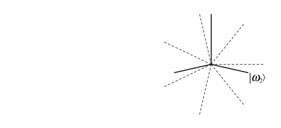
FIG. 3.: The two inequivalent optimal POVMs in the case of $M=7$. The POVM directions and input states are represented by thick and dashed lines respectively according to the conventions of Fig. 2.

Lemma 6 and theorem 2 may be used to provide a further variety of optimal $K$-element POVMs for ${\cal E}_{M}$ where $K$ is between 3 and $M$:

Lemma 7: Let ${\cal A}$ be any POVM as described in lemma 6 for which all angles $\theta_{a}$ have the form

$$\theta_{a}={\pi\over 2}+k_{a}{\pi\over M}\hskip 22.76219pt\mbox{where $k_{a}$ is an integer}$$ (79)

Then ${\cal A}$ is an optimal strategy for ${\cal E}_{M}$.

Proof: Since $I(\theta)$ is periodic with period ${\pi\over M}$ we have $I(\theta_{a})=I({\pi\over 2})$ for all $a$. Also $\sum\lambda_{a}^{2}=2$ so that Eq. (63) immediately gives $I({\cal E}_{M}:{\cal A})=I({\pi\over 2})$ i.e. ${\cal A}$ is optimal. 

Now note the following facts:
(a) All POVMs in theorem 2 satisfy Eq. (79).
(b) If ${\cal A}=\{\hat{A}_{i}\}$ is any POVM satisfying Eq. (79) then any $\mbox{Z}_{M}-$shifted version ${\cal A}_{l}$ of $\cal A$, defined for each $l\in\mbox{Z}_{M}$ by

$\displaystyle{\cal A}_{l}=\{\hat{V}^{l}\hat{A}_{i}\hat{V}^{\dagger l}\}$is a POVM also satisfying Eq. (79). (The angles $\theta_{a}$ are just shifted by ${l\pi\over M}$).
(c) If ${\cal A}_{1},\ldots,{\cal A}_{N}$ is any list of POVMs satisfying Eq. (79) then any convex combination of the ${\cal A}_{i}$’s will satisfy Eq. (79). (In forming convex combinations we naturally amalgamate POVM elements from different ${\cal A}_{i}$’s that lie in the same direction.)

Hence any convex combination of any $\mbox{Z}_{M}-$shifted versions of the POVMs in theorem 2 will be an optimal strategy. For example, let us consider a convex combination between two POVM’s in the case of $M$=5. The following $\{\hat{\omega}_{j}\}$ is one of the optimum detection strategies from theorem 2:

$$\hat{\omega}_{0} = (1-a^{2})(\hat{I}-\hat{\sigma}_{z}),$$ (81)

$$\hat{\omega}_{1} = {a^{2}\over 2}(\hat{I}-{\rm sin}({{4\pi}\over 5})\hat{\sigma}_{x}-{\rm cos}({{4\pi}\over 5})\hat{\sigma}_{z}),$$ (82)

$$\hat{\omega}_{2} = {a^{2}\over 2}(\hat{I}-{\rm sin}({{6\pi}\over 5})\hat{\sigma}_{x}-{\rm cos}({{6\pi}\over 5})\hat{\sigma}_{z}),$$ (83)

where $a^{2}=1/(2{\rm sin}^{2}{{2\pi}\over 5})$. The convex combination between $\{\hat{\omega}_{j}\}$ and $\{\hat{V}^{2}\hat{\omega}_{j}\hat{V}^{\dagger 2}\}$ forms the resolution of the identity

$$(1-\lambda)\sum_{j=0}^{2}\hat{\omega}_{j}+\lambda\sum_{k=0}^{2}\hat{V}^{2}\hat{\omega}_{k}\hat{V}^{\dagger 2}=\hat{I}\quad(\lambda\geq 0),$$ (84)

and we define

$$\hat{\mu}_{0} = (1-\lambda)\hat{\omega}_{0}+\lambda\hat{V}^{2}\hat{\omega}_{2}\hat{V}^{\dagger 2},$$ (86)

$$\hat{\mu}_{1} = (1-\lambda)\hat{\omega}_{1}+\lambda\hat{V}^{2}\hat{\omega}_{0}\hat{V}^{\dagger 2},$$ (87)

$$\hat{\mu}_{2} = (1-\lambda)\hat{\omega}_{2},$$ (88)

$$\hat{\mu}_{3} = \lambda\hat{V}^{2}\hat{\omega}_{1}\hat{V}^{\dagger 2}.$$ (89)

(Note that $\hat{\omega}_{0}\propto\hat{V}^{2}\hat{\omega}_{2}\hat{V}^{\dagger 2}$ and $\hat{\omega}_{1}\propto\hat{V}^{2}\hat{\omega}_{0}\hat{V}^{\dagger 2}$.) This gives a 4-element POVM $\{\hat{\mu}_{j}\}$ which maximizes the Shannon mutual information for ${\cal E}_{5}$.

The strategies in theorem 2 are not generally $\mbox{Z}_{M}-$covariant but they correspond to extreme points of $\cal P$. On the other hand the $\mbox{Z}_{M}-$covariant strategy of theorem 1 is generally not an extreme point of $\cal P$. The $\mbox{Z}_{M}$-covariant POVM of theorem 1 can be related to the asymmetrical 3-element POVM of theorem 2 as follows. Note first that if ${\cal W}=\{\hat{\omega}_{j}\}$ is any optimal POVM then so is $m{\cal W}=\{\hat{V}^{m}\hat{\omega}_{j}\hat{V}^{\dagger m}\}$ for any $m\in\mbox{Z}_{M}$. Indeed

$$I({\cal E}_{M}:{\cal W})=I({\cal E}_{M}:m{\cal W})$$ (90)

since the set of states of ${\cal E}_{M}$ is invariant under the action of $\mbox{Z}_{M}$. Given any one of the $N$ (=2, 3)-element POVMs $\{\hat{\omega}_{j}^{\ast}\}$ defined in theorem 2, one can consider the resolution of the identity

$${1\over M}\sum_{m=0}^{M-1}\sum_{j=0}^{N-1}\hat{V}^{m}\hat{\omega}_{j}^{\ast}\hat{V}^{\dagger m}=\hat{I}.$$ (91)

But the $MN$ elements $\{\hat{V}^{m}\hat{\omega}_{j}^{\ast}\hat{V}^{\dagger m}\}$ are proportional to each other in groups of $N$ and these groups may each naturally be summed and assigned a single element. This leads to the covariant $M$-element POVM which is just ${\cal A}_{M}$ of theorem 1 and lemma 3. In this sense ${\cal A}_{M}$ may be thought of as a convex combination

$\displaystyle{\cal A}_{M}=\sum_{k\in\mbox{Z}_{M}}{1\over M}k{\cal W}$where $\cal W$ is any one of the POVMs in theorem 2. If we know that ${\cal A}_{M}$ is optimal then Eqs. (90) and (4) will imply that $\cal W$ is optimal too. This provides an alternative proof of theorem 2 if we already know theorem 1 and lemma 3. On the other hand, if conversely we are given the result of theorem 2 (which uses lemma 3) then the accessible information of ${\cal E}_{M}$ must be $I({\pi\over 2})$ so ${\cal A}_{M}$ must be optimal (since $I({\cal E}_{M}:{\cal A}_{M})=I({\pi\over 2})$ by definition of $I(\theta)$ and ${\cal A}_{M}$).

V Implementation

The optimal POVMs ${\cal A}_{M}$ and ${\cal W}$ given in theorems 1 and 2, may be of interest from the viewpoint of putting quantum detection theory to the test. None of the POVMs for attaining maximum mutual information have been demonstrated by experiment yet. So far, only two kinds of optimal quantum detection scenarios have been confirmed experimentally. One is the Helstrom bound as the minimum average error probability [2], and the other is the Ivanovic-Dieks-Peres bound which gives the maximum probability for error-free detection, sometimes referred as the unambiguous measurement [13, 14, 15, 16]. (A concise review of both criteria can be found in ref. [17].) The former scenario was first demonstrated experimentally by Barnett and Riis [18]. The latter has been demonstrated in the laboratory by Huttner et al. [19]. Both of these are concerned with discrimination between binary nonorthogonal states. In our case of ${\cal A}_{M}$ and ${\cal W}$ for ${\cal E}_{M}$ with $M$ odd, we are dealing with essentially nonorthogonal measurement vectors in ${\cal H}_{2}$, which is called a generalized measurement. No von Neumann measurement can be an optimal strategy for ${\cal E}_{M}$ with $M$ odd. This case is of particular interest here. It is already well known that this kind of generalized measurement can be converted into a standard von Neumann measurement in a larger Hilbert space by introducing an ancillary system. This so-called Naimark extension ensures that any POVM can be physically implemented in principle [2, 3].

In this section we propose an optical scheme to demonstrate the optimal POVMs specified by ${\cal W}$ for ${\cal E}_{M}$ made of single mode photon polarization states. As seen in the previous section, ${\cal W}$ has three outcomes at most and suffices to provide an optimal strategy for all ${\cal E}_{M}$’s. For $M$ odd, it is always possible to find the optimal strategy with $m=n$, that is, $a^{2}=b^{2}=1/(2{\rm sin}^{2}{{m\pi}\over M})$ in theorem 2 if $m$ is taken as ${M\over 4}<m<{M\over 2}$. We consider the implementation of this particular detection strategy. The measurement vectors can be represented by

$$|\omega_{0}^{\ast}\rangle = -{\rm sin}{\gamma\over 2}|\downarrow\rangle,$$ (93)

$$|\omega_{1}^{\ast}\rangle = -{1\over{\sqrt{2}}}|\uparrow\rangle+{1\over{\sqrt{2}}}{\rm cos}{\gamma\over 2}|\downarrow\rangle,$$ (94)

$$|\omega_{2}^{\ast}\rangle = {1\over{\sqrt{2}}}|\uparrow\rangle+{1\over{\sqrt{2}}}{\rm cos}{\gamma\over 2}|\downarrow\rangle,$$ (95)

where

$${\rm cos}{\gamma\over 2}\equiv{\rm cot}{{m\pi}\over M},\quad{\rm sin}{\gamma\over 2}\equiv-\sqrt{1-{\rm cot}^{2}{{m\pi}\over M}},$$ (96)

and $|\uparrow\rangle$ and $|\downarrow\rangle$ are orthonormal bases of polarization. The first step is to make orthogonal measurement vectors by embedding $\{|\omega_{0}^{\ast}\rangle,|\omega_{1}^{\ast}\rangle,|\omega_{2}^{\ast}\rangle\}$ into a three or higher dimensional Hilbert space. One possible physical prescription is to make an optical circuit with two input ports, say, “a” and “b”. The signal state is guided into the port “a”, while the port “b” is initialized as the vacuum state. We can then consider the four dimensional Hilbert space spanned by the orthonormal basis $\{|E_{j}\rangle\}$,

$$|E_{0}\rangle \equiv |\uparrow\rangle_{a}|0\rangle_{b},$$ (98)

$$|E_{1}\rangle \equiv |\downarrow\rangle_{a}|0\rangle_{b},$$ (99)

$$|E_{2}\rangle \equiv |0\rangle_{a}|\uparrow\rangle_{b},$$ (100)

$$|E_{3}\rangle \equiv |0\rangle_{a}|\downarrow\rangle_{b},$$ (101)

where $|0\rangle$ is the vacuum state and the subscripts $a$ and $b$ indicate the port $``a"$ and $``b"$, respectively. A natural orthogonalization is

$$|\Omega_{0}\rangle \equiv |\omega_{0}^{\ast}\rangle_{a}|0\rangle_{b}+{\rm cos}{\gamma\over 2}|0\rangle_{a}|\uparrow\rangle_{b},$$ (103)

$$|\Omega_{1}\rangle \equiv |\omega_{1}^{\ast}\rangle_{a}|0\rangle_{b}+{1\over{\sqrt{2}}}{\rm sin}{\gamma\over 2}|0\rangle_{a}|\uparrow\rangle_{b},$$ (104)

$$|\Omega_{2}\rangle \equiv |\omega_{2}^{\ast}\rangle_{a}|0\rangle_{b}+{1\over{\sqrt{2}}}{\rm sin}{\gamma\over 2}|0\rangle_{a}|\uparrow\rangle_{b},$$ (105)

$$|\Omega_{3}\rangle \equiv |0\rangle_{a}|\downarrow\rangle_{b},$$ (106)

or equivalently,

$$|\Omega_{0}\rangle \equiv -{\rm sin}{\gamma\over 2}|\downarrow\rangle_{a}|0\rangle_{b}+{\rm cos}{\gamma\over 2}|0\rangle_{a}|\uparrow\rangle_{b},$$ (108)

$$|\Omega_{1}\rangle \equiv {1\over{\sqrt{2}}}\left(-|\uparrow\rangle_{a}|0\rangle_{b}+{\rm cos}{\gamma\over 2}|\downarrow\rangle_{a}|0\rangle_{b}+{\rm sin}{\gamma\over 2}|0\rangle_{a}|\uparrow\rangle_{b}\right),$$ (109)

$$|\Omega_{2}\rangle \equiv {1\over{\sqrt{2}}}\left(|\uparrow\rangle_{a}|0\rangle_{b}+{\rm cos}{\gamma\over 2}|\downarrow\rangle_{a}|0\rangle_{b}+{\rm sin}{\gamma\over 2}|0\rangle_{a}|\uparrow\rangle_{b}\right),$$ (110)

$$|\Omega_{3}\rangle \equiv |0\rangle_{a}|\downarrow\rangle_{b}.$$ (111)

It is easy to check that $\{|\Omega_{0}\rangle,|\Omega_{1}\rangle,|\Omega_{2}\rangle\}$ give the same channel matrix as $\{|\omega_{0}^{\ast}\rangle,|\omega_{1}^{\ast}\rangle,|\omega_{2}^{\ast}\rangle\}$, that is, $\langle\omega_{j}|\psi_{i}\rangle=\langle\Omega_{j}|(|\psi_{i}\rangle_{a}|0\rangle_{b})$ $(j=0,1,2)$. The second step is to decompose the von Neumann measurement $\{|\Omega_{j}\rangle\}$ into a unitary transformation followed by a measurement in the basis $\{|E_{j}\rangle\}$ in order to find a practical detector structure. We may write

$$\langle\Omega_{0}| \equiv \langle E_{2}|\hat{U}_{2}\hat{U}_{1},$$ (113)

$$\langle\Omega_{1}| \equiv \langle E_{1}|\hat{U}_{2}\hat{U}_{1},$$ (114)

$$\langle\Omega_{2}| \equiv \langle E_{0}|\hat{U}_{2}\hat{U}_{1},$$ (115)

$$\langle\Omega_{3}| \equiv \langle E_{3}|\hat{U}_{2}\hat{U}_{1},$$ (116)

where $\hat{U}_{1}$ and $\hat{U}_{2}$ are given by the matrices

$$\hat{U}_{1}\equiv\left(\begin{array}[]{cccc}1&0&0&0\cr 0&{\rm cos}{\gamma\over 2}&{\rm sin}{\gamma\over 2}&0\cr 0&-{\rm sin}{\gamma\over 2}&{\rm cos}{\gamma\over 2}&0\cr 0&0&0&1\end{array}\right),$$ (117)

$$\hat{U}_{2}\equiv\left(\begin{array}[]{cccc}{1\over\sqrt{2}}&{1\over\sqrt{2}}&0&0\cr-{1\over\sqrt{2}}&{1\over\sqrt{2}}&0&0\cr 0&0&1&0\cr 0&0&0&1\end{array}\right),$$ (118)

in the $\{|E_{0}\rangle,|E_{1}\rangle,|E_{2}\rangle,|E_{3}\rangle\}$ -basis representation. Eqs. (V) mean that in the detector, the signal state $|\psi_{i}\rangle_{a}|0\rangle_{b}$ is first transformed by $\hat{U}_{2}\hat{U}_{1}$, and is then measured in the basis $\{|E_{j}\rangle\}$ which corresponds to the simultaneous measurement with respect to which-path and which-polarization. The final step is to translate $\hat{U}_{2}\hat{U}_{1}$ into a practical circuit. In fact, this unitary transformation can be effected by the simple circuit consisting of passive linear optical devices such as polarizing beam splitters, polarization rotators, and halfwave plates [20]. The circuit is shown in Fig. 4. The $\hat{U}_{2}\hat{U}_{1}$ part consists of four halfwave plates, two polarizing beam splitters, and two polarization rotators. The polarization rotator represented by the circle with the rotation angle $\gamma$ performs

$$\hat{R}_{y}(\gamma)=\left(\begin{array}[]{cc}{\rm cos}{\gamma\over 2}&{\rm sin}{\gamma\over 2}\cr-{\rm sin}{\gamma\over 2}&{\rm cos}{\gamma\over 2}\end{array}\right).$$ (119)

The polarizing beam splitter represented by the square functions as a perfect mirror only for $\downarrow$-polarization (fast axis polarization). Light polarized along $\uparrow$-polarization (slow axis polarization) passes straight through it perfectly. The measurement $\{|E_{j}\rangle\}$ is made by photon counting at the four output ports. Note that only a single photon count at one of the three ports is expected and the outcome $|E_{3}\rangle$ is never expected. This structure is valid for any $M$ (the number of the signals) if one tunes the rotation angle $\gamma$ in $\hat{R}_{y}(\gamma)$ according to the value of $M$ (see Eq. (96)). The circuit is simple enough to be implemented with present technology.

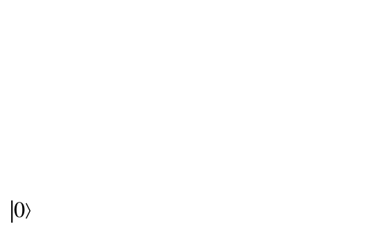
FIG. 4.: The optical circuit implementing ${\cal W}=\{\hat{\omega}_{0}^{\ast},\hat{\omega}_{1}^{\ast},\hat{\omega}_{2}^{\ast}\}$. It consists of the unitary transformation $\hat{U}_{2}\hat{U}_{1}$ followed by the measurement $\{|E_{j}\rangle\}$. $\hat{U}_{2}\hat{U}_{1}$ is effected by four halfwave plates, two polarizing beam splitters, and two polarization rotators. The measurement $\{|E_{j}\rangle\}$ is made by photon counting at the four output ports.

VI Concluding remarks

We have considered optimal strategies for symmetrical sources of real quantum states, treating in detail the sources ${\cal E}_{M}$ of $M$ real qubit states placed symmetrically in the $x-z$ plane around the Bloch sphere. Davies [5] has provided a general theorem characterising an optimal strategy for any $G$-covariant source whose group acts irreducibly on the whole state space. The symmetry group $\mbox{Z}_{M}$ of ${\cal E}_{M}$ does not act irreducibly on that state space so Davies’ theorem cannot be directly applied. However we proved an extension of this theorem which applies to $G$-covariant sources of real states for which the group acts irreducibly on the subset of real states (as is the case for ${\cal E}_{M}$). This led to a $\mbox{Z}_{M}$-covariant optimal strategy ${\cal A}_{M}$ for ${\cal E}_{M}$.

We also derived alternative optimal strategies ${\cal W}$ which contain at most three real POVM elements. In deriving this strategy ${\cal W}$ we exploited the convexity of $I(X:Y)$ on the convex set ${\cal P}$ of all POVMs. These strategies are not $G$-covariant in general but correspond to extreme points of ${\cal P}$. The small number of elements can be advantageous for practical implementation of the detection strategies as seen in the preceding section. The $G$-covariant strategy is not generally an extreme point of ${\cal P}$ but for higher dimensions it would seem easier to derive explicit $G$-covariant solutions rather than extreme point solutions.

Our results have added to the relatively small number of quantum sources for which optimal strategies are explicitly known. They may be extended in various straightforward ways (which we have omitted for clarity of presentation). For example the optimal strategies ${\cal A}_{M}$ and ${\cal W}$ for ${\cal E}_{M}$ remains optimal for the $M$-state source

$\displaystyle\{(1-\epsilon)\left|\psi_{k}\right\rangle\left\langle\psi_{k}\right|+\epsilon{1\over 2}\hat{I}_{2}:k\in\mbox{Z}_{M};{1\over M}\}$where each pure signal has been corrupted by noise given by the maximally mixed state ${1\over 2}\hat{I}_{2}$. This mixed state ensemble is clearly also $G$-covariant and the process of deriving the optimal strategy for this ensemble is quite the same as in the pure state case ($\epsilon=0$) but just multiplying the cosine terms in Eq. (17) by $(1-\epsilon)$. Then the same strategy remains optimal for the $G$-covariant mixed state ensemble although the accessible information decreases with $\epsilon$ as expected.

It is perhaps worth briefly contrasting our results of maximizing the mutual information with the problem of minimizing the average error probability. The latter is defined for ${\cal E}_{M}$ and any $M$-element POVM by

$$P_{\rm e}=1-{1\over M}\sum_{k=0}^{M-1}P(k|k).$$ (120)

The $P_{\rm e}$-optimal strategy is $\{\hat{\pi}_{k}\}=\{{2\over M}\left|\psi_{k}\right\rangle\left\langle\psi_{k}\right|:k\in\mbox{Z}_{M}\}$, that is, the POVM based on the state directions themselves. This is true also for the above mixed state ensemble. (The necessary and sufficient conditions for $P_{e}$-optimality, as given in [1, 2], are easily verified for $\{\hat{\pi}_{k}\}$.) Generally $P_{e}$-minimization is an essentially different type of optimization problem from $I(X:Y)$-maximization.

Within the confines of our formalism, various interesting issues remain unresolved. For example we would like to know an optimal strategy for the real $\mbox{Z}_{M}$-covariant source “double-${\cal E}_{M}$” in 4 dimensions comprising the 2-qubit signal states $\{\left|\psi_{k}\right\rangle\left|\psi_{k}\right\rangle:k\in\mbox{Z}_{M};{1\over M}\}$. In this case the symmetry group $\mbox{Z}_{M}$ does not act irreducibly even on the subset of all real 2-qubit states. Interesting properties of double-${\cal E}_{3}$ have been considered in [11] from the viewpoint of coding gain of transmittable information.

It is also a remaining difficult problem to optimize a quantum channel over both the a priori probability distribution of signals and the detection strategy for a fixed set of quantum states. The solution is known only for the binary pure state channel.

REFERENCES

[1]
A. S. Holevo, J. Multivar. Anal. 3, 337, (1973).
[2]
C. W. Helstrom : Quantum Detection and Estimation Theory
(Academic Press, New York, 1976).
[3]
A. Peres: Quantum Theory: concepts and methods, pp279-289,
(Kluwer Academic Publishers, Dortrecht, 1993).
[4]
T. Cover and J. Thomas : Elements of Information Theory
(John Wiley and Sons, New York, 1991).
[5]
E. B. Davies, IEEE Trans. Inf. Theory IT-24, 596 (1978).
[6]
C. A. Fuchs and A. Peres, Phys. Rev. A53, 2038 (1996).
[7]
M. Ban, K. Yamazaki, and O. Hirota, Phys. Rev. A55, 22 (1997).
[8]
M. Osaki, M. Ban, and O. Hirota, J. Mod. Opt. 45, 269 (1998).
[9]
A. S. Holevo, Probl. Peredachi Inform. vol 9, no. 2, 31 (1973).
[10]
P. Hausladen and W. K. Wootters, J. Mod. Opt. 41, 2385 (1994).
[11] A. Peres and W. Wootters, Phys. Rev. Lett. 66, 1119
(1992).
[12]
The authors are indebted to a private communication from A. S. Holevo
for the proof of Lemma 5.
[13]
I. D. Ivanovic, Phys. Lett. A123, 257 (1987).
[14]
D. Dieks, Phys. Lett. A126, 303 (1988).
[15]
A. Peres, Phys. Lett. A128, 19 (1988).
[16]
A. Chefles and S. M. Barnett, LANL Report No. quant-ph/9807023.
[17]
S. M. Barnett, Phil. Trans. R. Soc. Lond. A255, 2279 (1997).
[18]
S. M. Barnett and E. Riis, J. Mod. Opt. 44, 1061 (1997).
[19]
B. Huttner, A. Muller, J. D. Gautier, H. Zbinden, and N. Gisin,
Phys. Rev. A54, 3783 (1996).
[20]
N. J. Cerf, C. Adami, and P. G. Kwiat, Phys. Rev. A57, R1477
(1998).