Sampling Fourier Transforms on Different Domains
(Preliminary Version)

Abstract

We isolate and generalize a technique implicit in many quantum algorithms, including Shor’s algorithms for factoring and discrete log. In particular, we show that the distribution sampled after a Fourier transform over ${\mathbb{Z}}_{p}$ can be efficiently approximated by transforming over ${\mathbb{Z}}_{q}$ for any q in a large range. Our result places no restrictions on the superposition to be transformed, generalizing the result implicit in Shor which applies only to periodic superpositions. In addition, our proof easily generalizes to multi-dimensional transforms for any constant number of dimensions.

1 Introduction

One of the main applications of the fourier transform in quantum computing is finding a hidden subgroup of a finite abelian group. Specifically, we are given a finite abelian group $G$ and a function $f$ defined on $G$ that is constant and distinct on the cosets of some unknown subgroup $H$, which we must reconstruct.

The quantum algorithms solving this problem share a simple conceptual basis. Ideally, the machine is put into a uniform superposition of the elements of some coset of $H$. Then a fourier transform is performed, resulting in a uniform superposition on the quotient group $G/H$. The subgroup $H$ can be reconstructed after sampling this distribution. There have been many papers addressing special cases of this problem, including [Sim94], [Sho97], and [BL95]. These papers show how to recover the period of a periodic function defined on ${\mathbb{Z}}$, in other words they address the case where $H$ and $G$ are cyclic. [Kit95] solves a more general case, called the abelian stabilizer problem.

There is also great interest in extending these ideas to non-abelian groups, in part because the problem of graph isomorphism is reducible to finding a hidden subgroup in $S_{n}$. [Bea97] shows how compute a quantum fourier transform of a non-abelian group, but it is not known how to use this to find a hidden subgroup. In [EH98] an algorithm is given for finding the hidden subgroup of the dihedral group of order $2N$ that takes exponential time but has only polynomial query complexity.

In the abelian case, despite the simplicity of the conceptual framework, technical difficulties arise because it may be impossible to construct the desired initial superposition or to efficiently transform over the correct group, or to transform over the correct group at all if it is not given. In [Sim94] it is possible to transform over the group exactly, but these problems arise in [Sho97] and [BL95]. In the case of Shor’s discrete log algorithm, the correct group is known, but can only be efficiently transformed over if it is ${\mathbb{Z}}_{q}$ for a smooth integer $q$. [Kit95] gives an algorithm for fourier transforming over any abelian group. However, in the case of factoring, the ideal domain (that is, the group) is not even known: not only can the transform not be performed, but the exact input superposition cannot be constructed.

In [Sho97] and [BL95] these difficulties are resolved by transforming over smooth integers satisfying certain conditions, and providing technical arguments to show that the desired information can still be reconstructed. Unfortunately, these arguments seem particular to each algorithm and obscure the simple conceptual framework discussed above.

This paper unifies and generalizes these results. In particular, we prove that the distribution sampled after a Fourier transform over ${\mathbb{Z}}_{p}$ can be efficiently approximated by transforming over ${\mathbb{Z}}_{q}$ for any q in a large range. In addition, our proof easily generalizes to multi-dimensional transforms for any constant number of dimensions. This generalizes the previous work by removing any restrictions on the input distribution (such as periodicity) and unifying the proofs given for different dimensional transforms. From previous work it was not clear that the approach of transforming over a larger domain would always give the same points as the original set. Here we show that it does, and we work out the details one once and for all. Our result is in fact a mathematical property of the quantum fourier transform, which makes it easier to design algorithms. This also gives an alternative to Kitaev’s algorithm. Instead of using a more complicated quantum algorithm, the fourier transform is over a large enough, but otherwise arbitrary, domain. This would make it easy to, for example, always transform over a power of 2, while the conceptual anaylsis requires some other domain. Also, when the exact underlying group is not known, as is the case in factoring, algorithms can still be designed as if it were.

In summary, the following papers discuss computing fourier transforms efficiently. [Sho97] shows how to transform over smooth numbers. [Cle94] extends this to the case where the prime factors are not unique but still small. [Kit95] shows how to transform over any integer to within any epsilon. [Cop94] and [BEST96] show how to approximate the transform over the same integer by leaving out some gates. [Bea97] shows how to transform over the symmetric group. [MR96] gives classical algorithms for computing the fast fourier transform of functions defined on finite groups. [Høy97] gives quantum networks for computing unitary matrices that can be factored in the right way.

2 Definitions and Main Theorem

We will use the following notation throughout our discussion:

• $\boldsymbol{\alpha}$ is a fixed input superposition: $\boldsymbol{\alpha}=\sum_{i=0}^{p-1}\alpha_{i}|i\rangle$

• $\boldsymbol{\beta}$ is the fourier transform of $\boldsymbol{\alpha}$ over domain $p$: $\boldsymbol{\beta}=\sum_{i=0}^{p-1}\beta_{i}|i\rangle=\mbox{FT}_{p}(\boldsymbol{\alpha})$.

• $\boldsymbol{\gamma}$ is the fourier transform of $\boldsymbol{\alpha}$ over domain $q$, $q>p$: $\boldsymbol{\gamma}=\sum_{i=0}^{q-1}\gamma_{i}|i\rangle w=\mbox{FT}_{q}(\boldsymbol{\alpha})$.

Figures 1-3 give a simple example of these definitions:

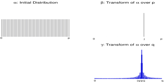
Figure 1: $\alpha$, Figure 2: $\beta$, and Figure 3: $\gamma$

Notice that the amplitude at $j$ in figure 2 is centered in figure 3 at the integers closest to $\frac{q}{p}j$. For this reason the next definition will also be useful:

• For a given index $i$, let $i^{\prime}$ denote $\lfloor\frac{q}{p}i\rfloor$. If $S\subseteq[p]$ is a set of indices, then $S^{\prime}\subseteq[q]$ is the set $\{\lfloor\frac{q}{p}s\rfloor|s\in S\}$.

• For $S\subseteq[p]$ and $\boldsymbol{\zeta}$ a vector of length p, let $\boldsymbol{\zeta}_{S}$ be the vector satisfying $(\boldsymbol{\zeta}_{S})_{i}=(\boldsymbol{\zeta})_{i}$ for all $i\in S$ and $(\boldsymbol{\zeta}_{S})_{i}=0$ otherwise.

• The $l_{1}$ norm of a vector $\boldsymbol{\zeta}$, denoted $\|\boldsymbol{\zeta}\|_{1}$, is $\sum_{i=0}^{\dim(\boldsymbol{\zeta})-1}|\zeta_{i}|$. Likewise the $l_{2}$ norm of a vector $\boldsymbol{\zeta}$, denoted $\|\boldsymbol{\zeta}\|_{2}$, is $\sqrt{\sum_{i=0}^{\dim(\boldsymbol{\zeta})-1}{|\zeta_{i}|^{2}}}$.

Finally, we need to define the following two distributions:

• ${\cal D}_{\boldsymbol{\beta}}$ is the distribution on $[p]$ induced by observing the superposition $\boldsymbol{\beta}$, i.e. ${\cal D}_{\boldsymbol{\beta}}(i)=|\beta_{i}|^{2}$.

• ${\cal D}_{\boldsymbol{\gamma}}$ is the distribution on $[p]$ given by ${\cal D}_{\boldsymbol{\gamma}}(i)=\frac{|\boldsymbol{\gamma}_{i^{\prime}}|^{2}}{\sum_{i\in[p]}|\gamma_{i^{\prime}}|^{2}}=\frac{|\boldsymbol{\gamma}_{i^{\prime}}|^{2}}{\|\boldsymbol{\gamma}_{[p]^{\prime}}\|^{2}}$. This is the distribution on $[p]$ induced by observing the superposition $\boldsymbol{\gamma}$, and outputting $i$ if the observation is of the form $i^{\prime}$ for some $i\in[p]$. Notice that if $q$ is a polynomial multiple of $p$ then we will see points of the form $i^{\prime}$ with significant probability and can round to find $i$. Thus this distribution can be reconstructed by sampling $\boldsymbol{\gamma}$.

We can now state our main theorem, which says that the distribution sampled after transforming over ${\mathbb{Z}_{p}}$ is close to a distribution which we can efficiently reconstruct by transforming over ${\mathbb{Z}_{q}}$ for $q$ a polynomial multiple of $p$.

Theorem 1

Let $p=O(2^{n^{k}})$ for some $k$. Then for any polynomial $s(n)$, there is a polynomial $t(n)$ such that whenever $q\geq t(n)p$,

$$\|{\cal D}_{\boldsymbol{\beta}}-{\cal D}_{\boldsymbol{\gamma}}\|_{1}\leq\frac{1}{s(n)}.$$

3 Applications

Theorem 1 simplifies proofs using fourier transforms. First we will indicate how to apply it in general and then we will give some specific applications.

3.1 General Application

A general approach to using the fourier transform is as follows:

• Show that some value $p$ exists such that when transforming over $p$, and sampling the resulting distribution, we see some set $S$ with at least 1/poly probability.

• Invoke the theorem for some $q$ which is a polynomial multiple larger than $p$ and which we can find and easily transform over, thereby reconstructing $S$.

Note that we place no requirements (such as periodicity) on the input distribution.

3.2 An Application

As an example of the application of our theorem, we reprove the following result of Shor:

Theorem 2

(Shor) Suppose the function $h:{\mathbb{Z}}\rightarrow{\mathbb{Z}}x$ is periodic with period $r$, one-to-one on its fundamental period, and efficiently computable. Then in random quantum polynomial time in $n=\log r$ it is possible to recover $r$.

Assume $h$ is as above. Suppose we could set up the superposition $\frac{1}{\sqrt{tr}}\sum_{i=0}^{tr}|i,h(i)\rangle$, transform over $tr$, and sample. Then we would see $(jt,b)$ with probability

$$\left|\frac{1}{tr}\sum_{i,h(i)=b}\omega_{tr}^{ijt}\right|^{2} = \left|\frac{1}{tr}\sum_{k=0}^{t-1}\omega_{tr}^{(i_{0}+kr)jt}\right|^{2}=\left|\frac{1}{r}\right|^{2}=\frac{1}{r^{2}}$$

where $i_{0}$ satisfies $h(i_{0})=b$ and $0\leq i_{0}<r$. To reconstruct the order $r$ we will need to sample $jt$ for $j$ relatively prime to $r$. The number of such $j$ is $\Phi(r)$, the number of distinct $b$ is $r$. Thus the probability of seeing a pair $(jt,b)$ with $j$ relatively prime to $r$ is $\frac{r\Phi(r)}{r^{2}}=\frac{\Phi(r)}{r}$. Since by a classical result in number theory $\frac{\Phi(r)}{r}>\frac{k}{\log\log r}$, this probability is at least $\frac{k}{\log n}$ for some constant $k$.

If we find $jt$ for $j$ relatively prime to $r$ we can compute $gcd(jt,tr)$ and $\frac{tr}{gcd(jt,tr)}=r$. Since we can check to make sure that this is actually the period, using the fact that $h$ is one-to-one on its fundamental domain, we can keep sampling until we see a pair of this form, which will happen with high probability within $O(\log(n))$ repetitions.

Unfortunately, since we do not know $r$, we can neither set up the desired input superposition nor transform over the desired domain. Assume for a moment that we could set up the input superposition $\frac{1}{\sqrt{tr}}\sum_{i=0}^{tr}|i,h(i)\rangle$ for some $t>r$. By our theorem, with $s(n)>2\log n$, there is a polynomial $t(n)$ so that if we transform over a smooth $q$ such that $t(n)tr<q<2t(n)tr$, then we will see an element of the form $s_{j}=\lfloor\frac{q}{tr}jt\rfloor$ with $j$ relatively prime to $r$ with probablity at least $\frac{1}{2t(n)\log n}$. Since

$$\left|s_{j}-\frac{qj}{r}\right|\leq 1\mbox{, we have }\left|\frac{s_{j}}{q}-\frac{j}{r}\right|\leq\frac{1}{q}.$$

Using the fact that $q>r^{2}$, by rounding $\frac{s_{j}}{q}$ to the nearest fraction with denominator less than $\sqrt{q}$, we will find $\frac{j}{r}$ and thus recover $r$. We can construct such a $q$ using the standard method of multiplying together succesively larger primes until we are in the correct range.

Finally, we must address the fact that we cannot actually construct the input superposition $\frac{1}{\sqrt{tr}}\sum_{i=0}^{tr}|i,h(i)\rangle$. But this problem is easily solved–we will construct a superposition which is exponentially close to the desired one. We can assume without loss of generality that we have an upper bound on $r^{\prime}$ on $r$ such that $r<r^{\prime}<2r$. (If not we can initially set $r^{\prime}=1$ then repeatedly run our algorithm, each time doubling our previous guess of $r^{\prime}$.) We can easily set up the superposition $\frac{1}{\sqrt{p}}\sum_{i=0}^{p}|i,h(i)\rangle$ where $p$ is a smooth number such that $(r^{\prime})^{2}<p<2(r^{\prime})^{2}$. This superposition is exponentially close to $\frac{1}{\sqrt{tr}}\sum_{i=0}^{tr}|i,h(i)\rangle$ where $tr$ is the multiple of $r$ nearest $p$.

3.3 An Application

As a second example of the application of our theorem, we reprove a result of Boneh and Lipton. Following their terminology, we say that the periodic function $h$ has order $m$ provided that no more than $m$ elements in the fundamental domain have the same image under $h$. Also, a function $f:{\mathbb{Z}}^{2}\rightarrow{\mathbb{Z}}$ has hidden linear structure over $q$ provided there is an integer $\alpha$ and a function $h:{\mathbb{Z}}\rightarrow{\mathbb{Z}}$ with period $q$ such that $f(x,y)=x+\alpha y$.

Theorem 3

(Boneh-Lipton) Suppose the function $f$ has hidden linear structure over q. Let $r$ be the smallest positive period of the underlying $h$ and assume $h$ has order at most $m$, where $m$ satisfies the following two conditions:

1. Let $n=\log r$, then $m$ is at most $n^{O(1)}$.

2. Let $p$ be the smallest prime divisor of $r$; then $m<p$.

Then, assuming $q$ and $m$ are known and $f$ is efficiently computable, in random quantum polynomial time in $n$ it is possible to recover the period $\alpha$.

The two conditions on $m$ are required so that the output of the algorithm can be tested for correctness.

We first need the following lemma. By using our theorem we are able to make do with this weakened version of the lemma found in Boneh-Lipton and considerably simplify the proof.

Lemma 1

For any integers $b_{1},\dots,b_{m}$, there are at least $r/m$ elements $x\in[r]$ satisfying

$$\left|\sum_{i=1}^{m}\omega_{r}^{xb_{i}}\right|\geq 1/2.$$

Proof: (of Lemma) Note that $\mbox{FT}_{r}\left(\sum_{i=1}^{m}\frac{1}{\sqrt{m}}|b_{i}\mod r\rangle\right)=\sum_{j=0}^{r-1}\frac{1}{\sqrt{r}}\left(\frac{1}{\sqrt{m}}\sum_{i=1}^{m}\omega_{r}^{xb_{i}}|j\rangle\right)$. Thus the number of $x$ satisfying the condition of the theorem is the same as the number of $x$ with amplitude at least $\frac{1}{2\sqrt{rm}}$ after this transform. Suppose there are at most $t$ such $x$’s. Note that the maximal amplitude after this transform is $\sqrt{\frac{m}{r}}$, thus

$$1\leq t\left(\sqrt{\frac{m}{r}}\right)^{2}+(r-t)\left(\frac{1}{2\sqrt{rm}}\right)^{2}$$

which implies

$$t\geq\frac{4rm-r}{4m^{2}-1}\geq\frac{r}{m},$$

as desired.  

Proof: (of Theorem) We first set up the superposition $\frac{1}{r}\sum_{x_{1},x_{2}}|x_{1},x_{2}\rangle$, then compute $f$, yielding

$$\frac{1}{r}\sum_{x_{1},x_{2}}|x_{1},x_{2},f(x_{1},x_{2})\rangle.$$

Suppose we could then transform over ${\mathbb{Z}}_{r}\times{\mathbb{Z}}_{r}$, sending for each $i\in\{1,2\}$, $x_{i}$ to $y_{i}$ with amplitude $\frac{1}{\sqrt{r}}\omega_{r}^{x_{i}y_{i}}$. Then we would see state $|y_{1},y_{2},b\rangle$ with probability

$$\left|\frac{1}{r^{2}}\sum_{x_{1},x_{2}:f(x_{1},x_{2})=b}\omega_{r}^{x_{1}y_{1}+x_{2}y_{2}}\right|^{2} = \left|\frac{1}{r^{2}}\sum_{t:f(t)=b}\sum_{x_{2}}\omega_{r}^{(t-\alpha x_{2})y_{1}+x_{2}y_{2}}\right|^{2}$$

$$= \left|\frac{1}{r^{2}}\sum_{t:f(t)=b}\omega_{r}^{ty_{1}}\sum_{x_{2}}\omega_{r}^{x_{2}(y_{2}-\alpha y_{1})}\right|^{2}$$

Thus if $y_{2}\equiv\alpha y_{1}\mod r$ and $\left|\sum_{t:f(t)=b}\omega_{r}^{ty_{1}}\right|^{2}>\frac{1}{4}$, we will see $|y_{1},y_{2},b\rangle$ with probability at least $\frac{1}{4r^{2}}$. There are at least $r/m$ distinct $b$’s, and, by our lemma, for each $b$ there are at least $r/m$ $y_{1}$’s satisfying the above condition. Thus we will see a triple of the form $|y,\alpha y\mod r,b\rangle$ with probability at least $\frac{1}{m^{2}}$.

Since we cannot necessarily transform over ${\mathbb{Z}}_{r}\times{\mathbb{Z}}_{r}$, we now use the two-dimensional version of our theorem with $s(n)=\frac{1}{2m^{2}}$ to say that there exists a polynomial $t(n)$ so that if we transform over ${\mathbb{Z}}_{q}\times{\mathbb{Z}}_{q}$ where $t(n)r<q<2t(n)r$ we will see triples of the form $|\lfloor\frac{qy}{r}\rfloor,\lfloor\frac{q\alpha y}{r}\rfloor,b\rangle$, with probability at least $\frac{1}{2m^{2}t(n)}$.

With such a triple in hand we can reconstruct a non trivial divisor of $\alpha$. First we find $\frac{y}{r}$ by rounding $\frac{\lfloor\frac{qy}{r}\rfloor}{q}$ to the nearest fraction with denominator $r$. Then we do the same for $\frac{\alpha y\mod r}{r}$. At this point we can proceed as outlined in [BL95].

Furthermore, as in [BL95], we can check to make sure that the triple sampled is of the above form and thus use recursion to solve our problem.  

4 Proof of Main Theorem

4.1 Outline

Recall that $\boldsymbol{\beta}=\mbox{FT}_{p}(\boldsymbol{\alpha})$ and $\boldsymbol{\gamma}=\mbox{FT}_{q}(\boldsymbol{\alpha})$ for some fixed superposition $\boldsymbol{\alpha}$.

The main goal of the proof is to show that if $q>t(n)p$ then for any set $S$ such that ${\cal D}_{\boldsymbol{\beta}}(S)$ is nonnegligible, ${\cal D}_{\boldsymbol{\gamma}}(S)$ is approximately ${\cal D}_{\boldsymbol{\beta}}(S)$. The closeness of the two distributions follows easily from this fact and is proved in section 5.3.

The central idea in the proof is to show the relationship between arbitrary $\boldsymbol{\beta}$ and the resulting $\boldsymbol{\gamma}$ by first analyzing the case in which $\boldsymbol{\beta}$ is a $\delta$-function, i.e, $\beta=|j\rangle$ for some $j\in[p]$. In this case $\boldsymbol{\gamma}$ is “almost” a $\delta$-function, i.e., its amplitude is highly concentrated at $j^{\prime}=\lfloor(q/p)j\rfloor$, and we can derive a lower bound on the amplitude located at $j^{\prime}$ and an upper bound on the amplitude located at any other primed index. These bounds are stated in Claim 1. We then extend the analysis from the case of $\delta$-functions to arbitrary $\boldsymbol{\beta}$ using linearity of the transform. This is the content of section 4.2.

There is a complication in proving the theorem however. To use the bounds derived from the $\delta$-functions, the amplitudes in $S$ must be approximately equal. Loosely speaking, in section 5.1 we show closeness of ${\cal D}_{\boldsymbol{\gamma}}(S)$ and ${\cal D}_{\boldsymbol{\beta}}(S)$ when the set satisfies this property (lemma 1), and in section 5.2 we split an arbitrary set $S$ into subsets with approximately equal amplitudes, apply the previous result to each subset, and combine the results (lemma 2).

4.2 Claim 1

To prove Lemma 2 we need to establish a relationship between the entries of $\boldsymbol{\beta}$ and the primed entries of $\boldsymbol{\gamma}$. In particular, we would like to have a lower bound on $|\gamma_{s^{\prime}}|$ in terms of $|\beta_{s}|$. Unfortunately, in general, $|\gamma_{s^{\prime}}|$ depends on all the entries of $\boldsymbol{\beta}$, not just on $\beta_{s}$. However, if $\boldsymbol{\beta}$ is a $\delta$-function, i.e. $\boldsymbol{\beta}=|j\rangle$ for some $j$, then, all other entries being $0$, $\boldsymbol{\gamma}_{j^{\prime}}$ does depend only on $\boldsymbol{\beta}_{j}$. Furthermore, we can use this case to derive the general relationship between $|\gamma_{s^{\prime}}|$ and the entries of $\boldsymbol{\beta}$. Thus we first make the following claim, whose proof can be found in the appendix:

Claim 1

Let $\sum_{i=0}^{q-1}\eta_{i}|i\rangle=\mbox{FT}_{q}\mbox{FT}^{-1}_{p}(|j\rangle)=\mbox{FT}_{q}\left(\sum_{i=0}^{p-1}\frac{1}{\sqrt{p}}\omega_{p}^{-ij}|i\rangle\right)$ for some $q>2p$ and $j\in[p]$. Then the following bounds hold:

• $|\eta_{j^{\prime}}|\geq\sqrt{\frac{p}{q}}\left(1-20\frac{p^{2}}{q^{2}}\right)$

• For $k\neq j$, $|\eta_{k^{\prime}}|\leq\sqrt{\frac{p}{q}}\frac{2}{|k-j|_{p}}\frac{p}{q}$

where $|x|_{p}=\left\{\begin{array}[]{ll}x\bmod p&\mbox{if $0\leq x\bmod p\leq p/2$}\\ -x\bmod p&\mbox{otherwise}\end{array}\right.$

This claim is again illustrated in Figures 1-3. It says that if one looks where the delta function goes if it is inverse transformed over $p$ and transformed over $q$, at the spot $j^{\prime}$ there will still be a large amplitude, and at any other $k^{\prime}$, the curves falls off at about 1 over the distance from $j^{\prime}$.

We can use our claim to derive a lower bound on $|\boldsymbol{\gamma}_{j^{\prime}}|$ given an arbitrary $\boldsymbol{\beta}$. We view $\boldsymbol{\beta}$ as a complex-weighted sum of $\delta$-functions, the $\delta$-function at $i$ receiving weight $\beta_{i}$. As in the claim, the amplitude $\gamma_{j^{\prime}}$ will receive a contribution of at least $|\beta_{j}|\sqrt{\frac{p}{q}}\left(1-20\frac{p^{2}}{q^{2}}\right)$ from the weighted $\delta$-function at $j$. On the other hand it will also receive a contribution of at most $|\beta_{k}|\sqrt{\frac{p}{q}}\frac{2}{|k-j|_{p}}\frac{p}{q}$ from the $\delta$-function at $k$ for each $k\neq j$. In the worst case these two types of contributions will be pointed in opposite directions, leading to a lower bound:

$$|\gamma_{j^{\prime}}|\geq|\beta_{j}|\sqrt{\frac{p}{q}}\left(1-20\frac{p^{2}}{q^{2}}\right)-\sum_{k\neq j}|\beta_{k}|\sqrt{\frac{p}{q}}\frac{2}{|k-j|_{p}}\frac{p}{q}.$$

More formally, by linearity of the transform, $\boldsymbol{\alpha}=\mbox{FT}^{-1}_{p}(\boldsymbol{\beta})=\mbox{FT}^{-1}_{p}\left(\sum_{j=0}^{p-1}\beta_{j}|j\rangle)\right)=\sum_{j=0}^{p-1}\beta_{j}\mbox{FT}^{-1}_{p}(|j\rangle)$, so $\boldsymbol{\gamma}=\mbox{FT}_{q}(\boldsymbol{\alpha})=\sum_{j=0}^{p-1}\beta_{j}\mbox{FT}_{q}(\mbox{FT}^{-1}_{p}(|j\rangle))$. Thus, for any particular $j$, we have

$$\gamma_{j^{\prime}}=\left(\sum_{k=0}^{p-1}\beta_{k}\mbox{FT}_{q}\left(\sum_{i=0}^{p-1}\frac{1}{\sqrt{p}}\omega_{p}^{-ij}|i\rangle\right)\right)_{j^{\prime}}=\beta_{j}\left(\mbox{FT}_{q}\left(\sum_{i=0}^{p-1}\frac{1}{\sqrt{p}}\omega_{p}^{-ij}|i\rangle\right)\right)_{j^{\prime}}+\sum_{k\neq j}\beta_{k}\left(\mbox{FT}_{q}\left(\sum_{i=0}^{p-1}\frac{1}{\sqrt{p}}\omega_{p}^{-ik}|i\rangle\right)\right)_{j^{\prime}}$$

By our claim, then,

$$|\gamma_{j^{\prime}}|\geq|\beta_{j}|\sqrt{\frac{p}{q}}\left(1-20\frac{p^{2}}{q^{2}}\right)-\sum_{k\neq j}|\beta_{k}|\sqrt{\frac{p}{q}}\frac{2}{|k-j|_{p}}\frac{p}{q}.$$ (1)

Since our goal is to establish that $\|\boldsymbol{\gamma}_{S^{\prime}}\|_{2}^{2}$ is approximately $\frac{p}{q}\|\boldsymbol{\beta}_{S}\|_{2}^{2}$, if we could show that, when q is chosen to be a sufficiently large polynomial multiple of p, the second of the two terms above is always negligible compared to the first, we would be done. Unfortunately, this is not true – there will in fact be indices $s$ with $|\beta_{s}|$ large where this second term entirely cancels the first. In particular, this can happen if there is an index $t$, close enough to $s$ that $\frac{2}{|t-s|_{p}}$ is not too small, whose amplitude, $|\beta_{t}|$, is more than a polynomial factor larger than $|\beta_{s}|$. But, there is not enough total amplitude in the superposition for this to happen at very many points in $S$. What we will show, then, is that there is a choice of q so that for a typical point in $S$ the second term in is negligible compared to the first, in other words, we can bound

$$\sum_{s\in S}\sum_{t\neq s}|\beta_{t}|\sqrt{\frac{p}{q}}\frac{2}{|t-s|_{p}}\frac{p}{q}.$$

The following argument and bound formalize the intuition that there is not enough total amplitude to wipe out most points in $S$:

Since,

$$\sum_{s\in S}\sum_{t\neq s}\frac{2}{|t-s|_{p}}|\beta_{t}| = \sum_{s\in S}\sum_{t\neq s,|\beta_{t}|\leq 1/\sqrt{|S|}}\frac{2}{|t-s|_{p}}|\beta_{t}|+\sum_{t,|\beta_{t}|>1/\sqrt{|S|}}|\beta_{t}|\sum_{s\in S,\neq t}\frac{2}{|t-s|_{p}}$$

$$\leq \left(\frac{1}{\sqrt{|S|}}\sum_{s\in S}4\ln p\right)+\left(4\ln p\sum_{t,|\beta_{t}|>1/\sqrt{|S|}}|\beta_{t}|\right)$$

$$\leq 8\sqrt{|S|}\ln p,$$

we have

$$\sum_{s\in S}\sum_{t\neq s}|\beta_{t}|\sqrt{\frac{p}{q}}\frac{2}{|t-s|_{p}}\frac{p}{q}\leq\left(\frac{p}{q}\right)^{3/2}8\sqrt{|S|}\ln p.$$ (2)

We will use both the numbered inequalities derived in this section in our proof of Lemma 2.

Acknowledgements: We thank Umesh Vazirani for many useful conversations.

5 Appendix

5.1 Proof of Lemma 2

Definition 1

A vector $\boldsymbol{\zeta}$ is called $\boldsymbol{\delta}$-uniform if for all $i,j$ such that $\boldsymbol{\zeta}_{i}$ and $\boldsymbol{\zeta}_{j}$ are both non-zero,

$$\delta\leq\frac{|\boldsymbol{\zeta}_{i}|}{|\boldsymbol{\zeta}_{j}|}\leq\frac{1}{\delta}$$

.

Lemma 2

Suppose that $\boldsymbol{\beta}_{S}$ is $\delta$-uniform and $\|\boldsymbol{\beta}_{S}\|_{2}^{2}=c$. Then if $q>\left(\frac{3200r\ln p}{\delta\sqrt{c}}\right)p$,

$$\|\boldsymbol{\gamma}_{S^{\prime}}\|_{2}^{2}\geq\frac{p}{q}\delta^{2}\left(1-\frac{1}{100r}\right)c.$$

Proof: (of Lemma 2)

We will lower bound $\|\boldsymbol{\gamma}_{S}\|_{1}$ in terms of $\|\boldsymbol{\beta}_{S}\|_{1}$. Then using $\delta$-uniformity $\|\boldsymbol{\beta}_{S}\|_{1}$ can be lower bounded in terms of $\|\boldsymbol{\beta}_{S}\|_{2}^{2}$. By a simple minimization principle, this gives a lower bound on $\|\boldsymbol{\gamma}_{S}\|_{2}^{2}$ in terms of $\|\boldsymbol{\beta}_{S}\|_{2}^{2}$, as desired.

Using Inequality 1 from the previous section we can derive the following lower bound on $\|\boldsymbol{\gamma}_{S^{\prime}}\|_{1}$:

$$\|\boldsymbol{\gamma}_{S^{\prime}}\|_{1} = \sum_{s\in S}|\gamma_{s^{\prime}}|$$

$$\geq \sum_{s\in S}\left(|\beta_{s}|\sqrt{\frac{p}{q}}\left(1-20\frac{p^{2}}{q^{2}}\right)-\sum_{t\neq s}|\beta_{t}|\sqrt{\frac{p}{q}}\frac{2}{|t-s|_{p}}\frac{p}{q}\right)$$

$$= \sqrt{\frac{p}{q}}\left(\left(1-20\frac{p^{2}}{q^{2}}\right)\|\boldsymbol{\beta}_{S}\|_{1}-\frac{p}{q}\sum_{s\in S}\sum_{t\neq s}\frac{2}{|t-s|_{p}}|\beta_{t}|\right)$$

Because $S$ is $\delta$-uniform, we can derive the following lower bound on the $l_{1}$-norm of $\|\boldsymbol{\beta}_{S}\|_{1}$:

$$\|\boldsymbol{\beta}_{S}\|_{1}\geq\frac{1+\delta}{\sqrt{2}\sqrt{1+\delta^{2}}}\sqrt{|S|}{\|\boldsymbol{\beta}_{S}\|_{2}}\geq\delta\sqrt{|S|}{\|\boldsymbol{\beta}_{S}\|_{2}},$$

where the first inequality comes from looking at the worst-case scenario (half the entries of $\boldsymbol{\beta}_{S}$ are of maximal size and the other half are of minimal size), and the second is just algebra.

Thus

$$\|\boldsymbol{\gamma}_{S^{\prime}}\|_{1}\geq\sqrt{\frac{p}{q}}\left(\left(1-20\frac{p^{2}}{q^{2}}\right)\delta\sqrt{|S|}{\|\boldsymbol{\beta}_{S}\|_{2}}-\frac{p}{q}\sum_{s\in S}\sum_{t\neq s}\frac{2}{|t-s|_{p}}|\beta_{t}|\right).$$

We upper bound the second term in this difference using Inequality 2 from the previous section:

$$\sum_{s\in S}\sum_{t\neq s}|\beta_{t}|\sqrt{\frac{p}{q}}\frac{2}{|t-s|_{p}}\frac{p}{q}\leq\left(\frac{p}{q}\right)^{3/2}8\sqrt{|S|}\ln p.$$

Thus,

$$\|\boldsymbol{\gamma}_{S^{\prime}}\|_{1} \geq \sqrt{\frac{p}{q}}\left(\left(1-20\frac{p^{2}}{q^{2}}\right)\delta\sqrt{|S|}{\|\boldsymbol{\beta}_{S}\|_{2}}-\frac{p}{q}8\sqrt{|S|}\ln p\right)$$

$$= \sqrt{\frac{p}{q}}\delta\sqrt{|S|}\sqrt{c}\left(\left(1-20\frac{p^{2}}{q^{2}}\right)-\frac{p}{q}\frac{8\ln p}{\delta\sqrt{c}}\right)$$

which implies that

$$\|\boldsymbol{\gamma}_{S^{\prime}}\|_{2}^{2}\geq\frac{p}{q}\delta^{2}c\left(1-20\frac{p^{2}}{q^{2}}-\frac{p}{q}\frac{8\ln p}{\delta\sqrt{c}}\right)^{2}.$$

Finally, using our assumption that $q>\left(\frac{3200r\ln p}{\delta\sqrt{c}}\right)p$,

$$\|\boldsymbol{\gamma}_{S^{\prime}}\|_{2}^{2}\geq\frac{p}{q}\delta^{2}c\left(1-\frac{1}{100r}\right),$$

as desired.  

5.2 Lemma 3

Using the bound for $\delta$-uniform sets in Lemma 2, we can establish the following bound for arbitrary sets $S$:

Lemma 3

If $\|\boldsymbol{\beta}_{S}\|_{2}^{2}=c$ and $q\geq\left(\frac{6400r\ln p\sqrt{\ln\frac{c}{|S|100r}}}{\sqrt{c\ln(1-\frac{1}{100r})}}\right)p$, then

$$\|\boldsymbol{\gamma}_{S^{\prime}}\|_{2}^{2}\geq\frac{p}{q}\left(1-\frac{1}{r}\right)c$$

Proof: (of Lemma 3 from Lemma 2)

Lemma 3 follows fairly easily from Lemma 2. The idea is to first remove from $S$ indices corresponding to insignificantly small amplitudes. Then partition the new $S$ into a collection of $\delta$-uniform subsets. We can apply Lemma 2 to each $\delta$-uniform subset of sufficiently large probability, and the total probability of the remaining, small $\delta$-uniform subsets is insignificant.

First, discard all indices in $s\in S$ with $|\beta_{s}|<\sqrt{\frac{c}{100r|S|}}$. Since we have thrown out at most $|S|$ such indices, we have lost at most $\frac{c}{100r}$ in probability and we have $\|\boldsymbol{\beta}_{S}\|_{2}^{2}\geq c\left(1-\frac{1}{100r}\right)$.

Partition $S$ into subsets

$$S_{i}=\{s\in S|\delta^{i}<|\beta_{s}|\leq\delta^{i-1}\}$$

for $0<i\leq\log_{1/\delta}\left(\sqrt{\frac{|S|100r}{c}}\right)$ and $\delta=(1-\frac{1}{100r})$.

In what follows let $T=\{i:\|\boldsymbol{\beta}_{S_{i}}\|_{2}^{2}\geq\frac{c}{log_{1/\delta}\sqrt{\frac{|S|100r}{c}}}\}$. Since

$$q\geq\left(\frac{6400r\ln p\sqrt{\ln\frac{c}{|S|100r}}}{\sqrt{c\ln(1-\frac{1}{100r})}}\right)p\geq\left(\frac{3200r\ln p}{\delta\sqrt{\min_{i\in T}\|\boldsymbol{\beta}_{S_{i}}\|_{2}^{2}}}\right)p,$$

we can apply Lemma 2 for each $i\in T$.

Thus,

$$\|\boldsymbol{\gamma}_{S^{\prime}}\|_{2}^{2} = \sum_{i}\|\boldsymbol{\gamma}_{S^{\prime}_{i}}\|_{2}^{2}$$

$$\geq \sum_{i\in T}\|\boldsymbol{\gamma}_{S^{\prime}_{i}}\|_{2}^{2}$$

$$\geq \sum_{i\in T}\frac{p}{q}\delta^{2}\|\boldsymbol{\beta}_{S_{i}}\|_{2}^{2}\left(1-\frac{1}{100r}\right)$$

$$= \frac{p}{q}\delta^{2}\left(\sum_{i\in T}\|\boldsymbol{\beta}_{S_{i}}\|_{2}^{2}+\sum_{i\notin T}\|\boldsymbol{\beta}_{S_{i}}\|_{2}^{2}\right)\left(1-\frac{1}{100r}\right)-\frac{p}{q}\delta^{2}\sum_{i\notin T}\|\boldsymbol{\beta}_{S_{i}}\|_{2}^{2}\left(1-\frac{1}{100r}\right)$$

$$= \frac{p}{q}\delta^{2}\left(\|\boldsymbol{\beta}_{S}\|_{2}^{2}\right)\left(1-\frac{1}{100r}\right)-\frac{p}{q}\delta^{2}\sum_{i\notin T}\|\boldsymbol{\beta}_{S_{i}}\|_{2}^{2}\left(1-\frac{1}{100r}\right)$$

Since $\|\boldsymbol{\beta}_{S}\|_{2}^{2}\geq c\left(1-\frac{1}{100r}\right)$ and

$$\sum_{i\notin T}\|\boldsymbol{\beta}_{S_{i}}\|_{2}^{2}\leq|T|\max_{i\notin T}\left(\|\boldsymbol{\beta}_{S_{i}}\|_{2}^{2}\right)\leq\log_{1/\delta}\left(\sqrt{\frac{|S|100r}{c}}\right)\frac{c}{log_{1/\delta}\sqrt{\frac{|S|100r}{c}}},$$

we have

$$\|\boldsymbol{\gamma}_{S^{\prime}}\|_{2}^{2} \geq \frac{p}{q}\delta^{2}c\left(1-\frac{1}{100r}\right)^{2}-\frac{p}{q}\delta^{2}\log_{1/\delta}\left(\sqrt{\frac{|S|100r}{c}}\right)\frac{c}{log_{1/\delta}\sqrt{\frac{|S|100r}{c}}}\left(1-\frac{1}{100r}\right)$$

$$= \frac{p}{q}c\delta^{2}\left(\left(1-\frac{1}{100r}\right)^{2}-\left(1-\frac{1}{100r}\right)\right)$$

$$\geq \frac{p}{q}c\left(1-\frac{1}{100r}\right)^{2}\left(\left(1-\frac{1}{100r}\right)^{2}-\left(1-\frac{1}{100r}\right)\right)$$

$$\geq \frac{p}{q}c\left(1-\frac{1}{r}\right),$$

as desired.  

5.3 Proof of Main Theorem from Lemma 3

Let $p=O(2^{n^{k}})$ and $s(n)$ be given. Let $t(n)=\frac{6400r\ln p\sqrt{\ln\frac{c}{|S|100r}}}{\sqrt{c\ln(1-\frac{1}{100r})}}$ with $r=4s(n)$ and $c=\frac{1}{2s(n)}$.

Let $R=\{i\in[p]:{\cal D}_{\boldsymbol{\beta}}(i)-{\cal D}_{\boldsymbol{\gamma}}(i)\geq 0\}$. Since

$$\|{\cal D}_{\boldsymbol{\beta}}-{\cal D}_{\boldsymbol{\gamma}}\|_{1} = \sum_{i\in[p]}\left|{\cal D}_{\boldsymbol{\beta}}(i)-{\cal D}_{\boldsymbol{\gamma}}(i)\right|$$

$$= \sum_{i\in R}\left({\cal D}_{\boldsymbol{\beta}}(i)-{\cal D}_{\boldsymbol{\gamma}}(i)\right)+\sum_{i\notin R}\left({\cal D}_{\boldsymbol{\gamma}}(i)-{\cal D}_{\boldsymbol{\beta}}(i)\right),$$

if $\|{\cal D}_{\boldsymbol{\beta}}-{\cal D}_{\boldsymbol{\gamma}}\|_{1}>\frac{1}{s(n)}$ then one of the above two sums must be at least $\frac{1}{2s(n)}$. Assume that $\sum_{i\in R}\left({\cal D}_{\boldsymbol{\beta}}(i)-{\cal D}_{\boldsymbol{\gamma}}(i)\right)>\frac{1}{2s(n)}$. Then since $\sum_{i\in R}|\beta_{i}|^{2}>\frac{1}{2s(n)}$, we can apply Lemma 1 with $r=4s(n)$ and $c=\sum_{i\in R}|\beta_{i}|^{2}>\frac{1}{2s(n)}$. Note also that $\|\boldsymbol{\gamma}_{[p]^{\prime}}\|^{2}_{2}\leq\frac{p}{q}$, thus

$$\sum_{i\in R}\left({\cal D}_{\boldsymbol{\beta}}(i)-{\cal D}_{\boldsymbol{\gamma}}(i)\right) = \|\boldsymbol{\beta}_{R}\|_{2}^{2}-\frac{\|\boldsymbol{\gamma}_{R^{\prime}}\|_{2}^{2}}{\|\boldsymbol{\gamma}_{[p]^{\prime}}\|_{2}^{2}}$$

$$\leq \|\boldsymbol{\beta}_{R}\|_{2}^{2}-\left(\frac{p}{q}\left(1-\frac{1}{4s(n)}\right)\frac{\|\boldsymbol{\beta}_{R}\|_{2}^{2}}{\|\boldsymbol{\gamma}_{[p]^{\prime}}\|_{2}^{2}}\right)$$

$$\leq \|\boldsymbol{\beta}_{R}\|_{2}^{2}\frac{1}{4s(n)}$$

$$\leq \frac{1}{2s(n)},$$

a contradiction, as desired.

On the other hand, if $\sum_{i\notin R}\left({\cal D}_{\boldsymbol{\gamma}}(i)-{\cal D}_{\boldsymbol{\beta}}(i)\right)>\frac{1}{2s(n)}$ then again applying lemma 1 and using the fact that $\|\boldsymbol{\gamma}_{R^{\prime}}\|_{2}^{2}\leq\frac{p}{q}\|\boldsymbol{\beta}_{R}\|_{2}^{2}$,

$$\sum_{i\notin R}\left({\cal D}_{\boldsymbol{\gamma}}(i)-{\cal D}_{\boldsymbol{\beta}}(i)\right) = \frac{\|\boldsymbol{\gamma}_{R^{\prime}}\|_{2}^{2}}{\|\boldsymbol{\gamma}_{[p]^{\prime}}\|_{2}^{2}}-\|\boldsymbol{\beta}_{R}\|_{2}^{2}$$

$$\leq \frac{\frac{p}{q}\|\boldsymbol{\beta}_{R}\|_{2}^{2}}{\frac{p}{q}\left(1-\frac{1}{4s(n)}\right)\|\boldsymbol{\beta}_{[p]}\|_{2}^{2}}-\|\boldsymbol{\beta}_{R}\|_{2}^{2}$$

$$= \|\boldsymbol{\beta}_{R}\|_{2}^{2}\left(\frac{1}{1-\frac{1}{4s(n)}}-1\right)$$

$$\leq \frac{1}{2s(n)},$$

also a contradiction.

5.4 Proof of Claim

Claim 1 Let $\sum_{i=0}^{q-1}\eta_{i}|i\rangle=\mbox{FT}_{q}\left(\sum_{i=0}^{p-1}\frac{1}{\sqrt{p}}\omega_{p}^{-ij}|i\rangle\right)$ for some $q>2p$ and $j\in[p]$. Then the following bounds hold:

1. $|\eta_{j^{\prime}}|\geq\sqrt{\frac{p}{q}}\left(1-20\frac{p^{2}}{q^{2}}\right)$

2. For $k\neq j$, $|\eta_{k^{\prime}}|\leq\sqrt{\frac{p}{q}}\frac{2}{|k-j|_{p}}\frac{p}{q}$

where $|x|_{p}=\left\{\begin{array}[]{ll}x\bmod p&\mbox{if $0\leq x\bmod p\leq p/2$}\\ -x\bmod p&\mbox{otherwise}\end{array}\right.$

Proof: The first bound is established as follows:

For some $\epsilon$ satisfying $0\leq\epsilon<1$,

$$\eta_{j^{\prime}} = \frac{1}{\sqrt{q}}\sum_{i=0}^{p-1}\frac{1}{\sqrt{p}}\omega_{p}^{-ij}\omega_{q}^{i(jq/p+\epsilon)}$$

$$= \frac{1}{\sqrt{q}}\sum_{i=0}^{p-1}\frac{1}{\sqrt{p}}\omega_{p}^{-ij}\omega_{p}^{ij}\omega_{q}^{i\epsilon}$$

$$= \sqrt{\frac{p}{q}}\frac{1}{p}\sum_{i=0}^{p-1}\omega_{q}^{i\epsilon}$$

Since $\left|\frac{1}{p}\sum_{i=0}^{p-1}\omega_{p}^{i\epsilon p/q}\right|\geq\cos(2\pi\epsilon p/q)\geq 1-\frac{(2\pi\epsilon p/q)^{2}}{2}\geq 1-20(p/q)^{2}$, we have $|\eta_{j^{\prime}}|\geq\sqrt{\frac{p}{q}}\left(1-20\frac{p^{2}}{q^{2}}\right)$, as desired.

The second bound requires the following observation:

Observation 1

Let $\delta=|x-\lfloor x\rceil|$. Then $\left|\frac{1}{p}\sum_{i=0}^{p-1}\omega_{p}^{ix}\right|\leq\frac{\delta}{|x|_{p}}$, whenever the latter expression is defined.

Using this observation we can prove the second bound as follows:

For some $\epsilon$ satisfying $0\leq\epsilon<1$,

$$\eta_{k^{\prime}} = \frac{1}{\sqrt{q}}\sum_{i=0}^{p-1}\frac{1}{\sqrt{p}}\omega_{p}^{-ij}\omega_{q}^{i(kq/p+\epsilon)}$$

$$= \sqrt{\frac{p}{q}}\frac{1}{p}\sum_{i=0}^{p-1}\omega_{p}^{i(k-j+\epsilon\frac{p}{q})}$$

Using our observation, with $\delta=\min(\epsilon\frac{p}{q},1-\epsilon\frac{p}{q})$, and the fact that $q>2p$, we have $|\eta_{k^{\prime}}|\leq\sqrt{\frac{p}{q}}\frac{\delta}{|k-j+\epsilon\frac{p}{q}|_{p}}\leq\sqrt{\frac{p}{q}}\frac{2}{|k-j|_{p}}\frac{p}{q}$, as desired.  

Proof: (of observation) Since $\left|\sum_{i=0}^{p-1}\omega_{p}^{ix}\right|=\left|\sum_{i=0}^{p-1}\omega_{p}^{i|x|_{p}}\right|$, we will bound the latter sum instead. For ease of reading, let $y=|x|_{p}$ in what follows. Note that $\delta=|x-\lfloor x\rceil|=|y-\lfloor y\rceil|$.

First we rewrite each vector in the sum $\sum_{i=0}^{p-1}\omega_{p}^{iy}$ as an integral over an arc of a circle, in particular, we substitute $\frac{p}{\pi y}\int_{iy-y/2}^{iy+y/2}\omega_{p}^{t}dt$ for $\omega_{p}^{iy}$. Then

$$\left|\sum_{i=0}^{p-1}\omega_{p}^{iy}\right| = \left|\frac{p}{\pi y}\sum_{i=0}^{p-1}\int_{iy-y/2}^{iy+y/2}\omega_{p}^{t}dt\right|$$

$$= \left|\frac{p}{\pi y}\int_{-y/2}^{(p-1)y+y/2}\omega_{p}^{t}dt\right|$$

$$= \left|\frac{p}{\pi y}\int_{-y/2}^{yp-y/2}\omega_{p}^{t}dt\right|$$

$$= \left|\frac{p}{\pi y}\int_{0}^{yp}\omega_{p}^{t}dt\right|$$

$$= \left|\frac{p}{\pi y}\left(\int_{0}^{\lfloor y\rceil p}\omega_{p}^{t}dt+\int_{\lfloor y\rceil p}^{yp}\omega_{p}^{t}dt\right)\right|$$

$$= \left|\frac{p}{\pi y}\int_{\lfloor y\rceil p}^{yp}\omega_{p}^{t}dt\right|$$

$$= \left|\frac{p}{\pi y}\int_{0}^{\delta p}\omega_{p}^{t}dt\right|$$

$$= \frac{p\delta}{y}$$

Thus $\left|\frac{1}{p}\sum_{i=0}^{p-1}\omega_{p}^{ix}\right|\leq\frac{\delta}{|x|_{p}}$, as desired.

 

5.5 Multiple Dimensions

A analogous proof can be given in the case of multi-dimensional Fourier transforms. First we need to define

• $\boldsymbol{\beta}=\sum_{\vec{x}\in\prod[{p_{i}}]}\beta_{\vec{x}}|\vec{x}\rangle=\bigotimes_{0\leq i\leq k}\mbox{F}T_{p_{i}}(\boldsymbol{\alpha})$ for some superposition $\boldsymbol{\alpha}$,

• $\boldsymbol{\gamma}=\sum_{\vec{x}\in\prod[{q_{i}}]}\gamma_{\vec{x}}|\vec{x}\rangle$ is $\bigotimes_{0\leq i\leq k}\mbox{F}T_{q_{i}}(\boldsymbol{\alpha})$, and

• $S^{\prime}=\{(\lfloor\frac{q_{1}}{p_{1}}s_{1}\rceil,\lfloor\frac{q_{2}}{p_{2}}s_{2}\rceil,\dots,\lfloor\frac{q_{k}}{p_{k}}s_{k}\rfloor|(s_{1},s_{2},\dots,s_{k})\in S\}$. Likewise $\vec{y}^{\prime}$ satisfies $(\vec{y}^{\prime})_{i}=\lfloor\frac{q_{i}}{p_{i}}(\vec{y})_{i}\rfloor$.

Now we can assert the following lemma which is the multidimensional version of our Lemma 2:

Lemma 4

If $\|\boldsymbol{\beta}_{S}\|_{2}^{2}=c$ for some set $S\subseteq\prod[{p_{i}}]$, and for all i, $q_{i}>\left(\frac{2^{k+2}k^{k+1}800r(\ln p)^{k}\sqrt{\ln\frac{c}{|S|100r}}}{\sqrt{c\ln(1-\frac{1}{100r})}}\right)p_{i}$, then $\|\boldsymbol{\gamma}_{S^{\prime}}\|_{2}^{2}\geq(\prod_{i=1}^{i=k}{\frac{p_{i}}{q_{i}}})\left(1-\frac{1}{r}\right)c$.

Notice that the quantity in parentheses is a polynomial whenever $k$, the number of dimensions is constant. Using this lemma we can prove the multidimensional version of our theorem precisely as we did in the one dimensional case.

To prove the above lemma we will need a generalization of our Claim 1. In what follows let $\mbox{FT}_{\vec{p}}=\bigotimes_{0\leq i\leq k}\mbox{F}T_{p_{i}}$ and $\mbox{FT}_{\vec{q}}=\bigotimes_{0\leq i\leq k}\mbox{F}T_{q_{i}}$.

Claim 2

Let $\boldsymbol{\zeta}$ satisfy $\mbox{FT}_{\vec{p}}(\boldsymbol{\zeta})=|\vec{y}\rangle$ for some $\vec{y}\in\prod[{p_{i}}]$. Let $\sum_{\vec{x}\in\prod[{q_{i}}]}\eta_{\vec{x}}|\vec{x}\rangle=\mbox{FT}_{\vec{q}}\left(\boldsymbol{\zeta}\right)$ for some $q_{i}$ such that for all $i$, $q_{i}>2p_{i}$. Then the following bounds hold:

1. $|\eta_{\vec{y}^{\prime}}|\geq\prod_{i=1}^{i=k}\sqrt{\frac{p_{i}}{q_{i}}}\left(1-20\frac{p_{i}^{2}}{q_{i}^{2}}\right)$

2. For $\vec{z}\neq\vec{y}$, $|\eta_{\vec{z}^{\prime}}|\leq\left(\prod_{i=1}^{i=k}\sqrt{\frac{p_{i}}{q_{i}}}\right)\left(\prod_{j,\vec{z}_{j}\neq\vec{y}_{j}}\frac{2}{|\vec{z}_{j}-\vec{y}_{j}|_{p}}\frac{p_{j}}{q_{j}}\right)$

This claim, as in the one dimensional case, allows us to give the following lower bound on $|\boldsymbol{\gamma}_{\vec{x}^{\prime}}|$:

$$|\gamma_{\vec{x}^{\prime}}|\geq|\beta_{\vec{x}}|\prod_{i=1}^{i=k}\sqrt{\frac{p_{i}}{q_{i}}}\left(1-20\frac{p_{i}^{2}}{q_{i}^{2}}\right)-\sum_{\vec{z}\neq\vec{x}}|\beta_{\vec{z}}|\left(\prod_{i=1}^{i=k}\sqrt{\frac{p_{i}}{q_{i}}}\right)\left(\prod_{j,\vec{z}_{j}\neq\vec{x}_{j}}\frac{2}{|\vec{z}_{j}-\vec{x}_{j}|_{p}}\frac{p_{j}}{q_{j}}\right).$$

As in the proof of the one dimensional case, we will need to upper bound the following quantity:

$$\sum_{\vec{x}\in S}\sum_{\vec{z}\neq\vec{x}}|\beta_{\vec{z}}|\left(\prod_{j,\vec{z}_{j}\neq\vec{x}_{j}}\frac{2}{|\vec{z}_{j}-\vec{x}_{j}|_{p}}\frac{p_{j}}{q_{j}}\right).$$

Using an argument which is analogous to the one-dimensional case we get a bound of

$$2^{k+2}k^{k+1}\sqrt{|S|}(\ln p)^{k}\min_{i}\{\frac{p_{i}}{q_{i}}\}$$

Using this bound we can carry out the rest of the proof precisely as in the one dimensional case to get the factors specified in Lemma 4.

References

- [Bea97] Robert Beals. Quantum computation of Fourier transforms over symmetric groups. In Proceedings of the Twenty-Ninth Annual ACM Symposium on Theory of Computing, pages 48–53, El Paso, Texas, 4–6 May 1997.
- [BEST96] Adriano Barenco, Artur K. Ekert, Kalle-Antti Suominen, and Päivi Törmä. Appriximate quantum Fourier transform and decoherence. Submitted to Physical Review A, January 1996.
- [BL95] Dan Boneh and Richard J. Lipton. Quantum cryptanalysis of hidden linear functions (extended abstract). In Don Coppersmith, editor, Advances in Cryptology—CRYPTO ’95, volume 963 of Lecture Notes in Computer Science, pages 424–437. Springer-Verlag, 27–31 August 1995.
- [Cle94] Richard Cleve. A note on computing fourier transforms by quantum programs. 1994.
- [Cop94] D. Coppersmith. An approximate fourier transform useful in quantum factoring. Technical Report RC19642, IBM, 1994.
- [EH98] Mark Ettinger and Peter Høyer. On quantum algorithms for noncommutative hidden subgroups. May 1998.
- [Høy97] Peter Høyer. Efficient quantum transforms. February 1997.
- [Kit95] Alexey Yu. Kitaev. Quantum measurements and the abelian stabilizer problem. 1995.
- [MR96] David K. Maslen and Daniel N. Rockmore. Generalized FFTS - A Survey of Some Recent Results. Technical Report PCS-TR96-281, Dartmouth College, Computer Science, Hanover, NH, April 1996.
- [Sho97] Peter W. Shor. Polynomial-time algorithms for prime factorization and discrete logarithms on a quantum computer. SIAM Journal on Computing, 26(5):1484–1509, October 1997.
- [Sim94] Daniel R. Simon. On the power of quantum computation. In 35th Annual Symposium on Foundations of Computer Science, pages 116–123, Santa Fe, New Mexico, 20–22 November 1994. IEEE.