Two-photon Franson-type interference experiments are not tests of local realism

Abstract

We report a local hidden-variable model which reproduces quantum predictions for the two-photon interferometric experiment proposed by Franson [Phys. Rev. Lett. 62, 2205 (1989)]. The model works for the ideal case of full visibility and perfect detection efficiency. This result changes the interpretation of a series of experiments performed in the current decade.

The ingenious two-particle interferometer introduced by Franson [4] is an exciting tool to reveal properties of entangled states. In the current decade this device was used in many two-photon interferometric experiments [5], that beautifully reveal complementarity between single and two-photon interference. The results of the experiments cannot be described using standard methods involving classical electromagnetic fields [6].

However, in the original paper, entitled Bell Inequality for Position and Time, and in many papers that followed, it was claimed that the experiment constitutes a “test of local realism involving time and energy”. Some authors were more sceptical, noting that even the ideal gedanken model of the experiment involves a postselection procedure, in which $50\%$ of the events are discarded when computing the correlation functions [7]. If all events are taken into account standard Bell inequalities are not violated. This does not prove the existence of a local hidden-variable (LHV) model, but merely states that such a model is not ruled out.

The situation is made even less transparent by similar claims concerning certain two-photon polarization experiments [8] where the problem of discarded events also appears. This has earlier been treated on equal footing with the problems of the Franson-type experiments, but a recent analysis in [9] of the entire pattern of events in the experiments in [8] reestablishes the unconditional violation of local realism. One could be tempted to adapt the procedure of [9] to the Franson experiment, but as will be shown below, this is not possible.

In short, no one has been able to explicitly show an unconditional incompatibility of local realistic models of Franson experiments with the quantum mechanical predictions, but on the other hand, no one has thus far shown the existence of a LHV model for such predictions [10, 11]. Our aim is to resolve this uncertainty about the interpretation of the Franson interferometry by constructing a LHV model which fully reproduces the quantum predictions for the ideal case, i.e for $100\%$ efficient detectors and $100\%$ visibility of the two-particle interference.

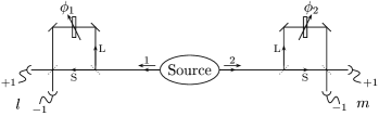
FIG. 1.: The generic setup of the Franson two-photon interference experiment.

First, let us describe the main idea behind the Franson type experiments. The two-particle interferometer is presented schematically in Fig. 1. In the actual experiments the source of the photon pairs was the process of spontaneous parametric down conversion (PDC) in a nonlinear crystal pumped by a monochromatic cw laser field. Both the photon traveling to the left as well as the one traveling to the right were fed into two identical unbalanced Mach-Zehnder interferometers [12]. The difference of the optical paths in those interferometers, $\Delta L$, satisfies the relation $cT_{\text{coh}}\ll\Delta L$, where $c$ is the speed of light and $T_{\text{coh}}$ is the coherence time of the down-converted photons (it is effectively defined by the filters and the geometry of the collection of the PDC radiation). Such optical path differences prohibit any single photon interference. However, two-particle interference is observable, provided there is no way to know the actual paths of the photons of a pair which caused two spatially separated detectors to click.

The down-converted photons have the property that their detection times (barring retardation effects) are correlated to within their coherence times [13]. Thus, the two photons either cause clicks in the two detection stations which are either coincident (i.e., within coherence times), or one of the clicks is delayed with respect to the other one by a time difference of the order $\Delta L/c$. In the second case, one has the full “which way” information about the process that caused the two clicks (one knows exactly which photon went via the longer path, and which via the shorter one). In the first case, however, either both went via the longer arms (denoted by $L$) or both via the shorter arms ($S$) of the local interferometers. Therefore, provided the time of emission is unknown [14], there is no way to distinguish the two processes, and thus they interfere. The relative phase of the quantum amplitudes for the two processes can be controlled by the phase shifters within the Mach-Zehnder interferometers, and is equal to their sum.

Formally this can be described in the following simple way. Right before the exit beamsplitters of the local interferometers (Fig. 1) the photon state is

$$\textstyle|\psi\rangle_{12}=\frac{1}{2}\bigl{(}|S\rangle_{1}+e^{i\phi_{1}}|L\rangle_{1}\bigr{)}\bigl{(}|S\rangle_{2}+e^{i\phi_{2}}|L\rangle_{2}\bigr{)}.$$ (1)

The state vector $|S\rangle_{n}$ represents the $n$-th photon in the shorter arm, and $L$ denotes the longer arm. The detectors are located behind the exit 50–50 beamsplitters, and thus they hide the direct information about the path of a photon (the indirect information can still be revealed by the detection times). The part of the state vector $|\psi\rangle_{12}$ responsible for coincident events (up to $T_{\text{coh}}$) is given by

$$\textstyle\frac{1}{2}\bigl{(}|S\rangle_{1}|S\rangle_{2}+e^{i(\phi_{1}+\phi_{2})}|L\rangle_{1}|L\rangle_{2}\bigr{)}.$$ (2)

As long as the emission times of the pairs of photons are in principle undefined, the two terms can interfere [14]. The norm of this component is $1/\sqrt{2}$, and thus only half of the events will belong to this class. If the exit 50–50 beamsplitters are symmetric, the probabilities for two-particle processes to give the result $l=\pm 1$ for particle 1 and the result $m=\pm 1$ for particle 2, under specified phase settings, and in coincidence, are

$$P\bigl{(}l;m(\text{coincidence})|\phi_{1},\phi_{2}\bigr{)}$$ (3)

$$\qquad=\textstyle\frac{1}{8}\bigl{(}1+lm\cos(\phi_{1}+\phi_{2})\bigr{)}.$$ (4)

The other terms of $|\psi\rangle_{12}$ cannot lead to coincident counts, and because the paths taken by the photons is exactly known there is no interference. The probabilities are

$$P(l,\text{L};m,\text{E}|{\phi_{1}},{\phi_{2}})=P(l,\text{E};m,\text{L}|{\phi_{1}},{\phi_{2}})=\textstyle\frac{1}{16},$$ (5)

where E denotes an earlier count, and L denotes a later count. No single photon interference is observed, in other words

$$\textstyle P(l|{\phi_{1}})=P(m|{\phi_{2}})=\frac{1}{2}.$$ (6)

An essential property of any deterministic LHV model for the experiment is that it should contain the emission time as one of the variables describing the experiment. The reason is that the beamsplitters of, say, the right interferometer may be removed at any moment of the measurement process. In this case, the photons would be detected solely by the detector $+1$, and the detection time would indicate the moment of emission (of course, only up to the coherence time, but this is not essential). I.e., there exist an operational situation in which the emission time can be measured, and therefore it must be included in the LHV model. Further, under the same operational situation, the detections behind the left interferometer are either coincident with the detections on the right side, or retarded by $\Delta L/c$. The LHV model must give predictions for the local events at one side of the experiment, independent of what measuring device is used at the other side. I.e., it must predict whether a given count on the left side would be coincident (we shall call this an early detection) or delayed (a late detection) with respect to a count at the right side, when the right interferometer is dismantled. From now on we shall assume, just like in the quantum model, that the average time between emissions is much longer than all other characteristic times of the experiment. Otherwise, we assume it to be completely random.

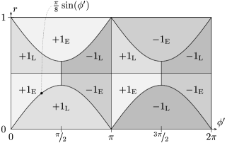
FIG. 2.: LHV model for the detection at the left station. For a detailed description see the main text. The areas labeled $\pm 1$ indicate detections at the $\pm 1$ detector, whereas E or L indicate early or late detections. The lower curve in the left side of the chart is given by $\frac{\pi}{8}\sin{\phi^{\prime}}$, and the shape of the other curves can be easily established by the evident symmetries of the chart.

Let us now present a LHV model for a single emission at a specific time for the Franson experiment. The hidden variables are chosen to be an angular coordinate $\phi\in[0,2\pi]$ and an additional coordinate $r\in[0,1]$. The ensemble of hidden variables is chosen as that of an even distribution in this rectangle in $(\phi,r)$-space, but each pair of particles is described by a definite point $(\phi,r)$ in the rectangle, defined at the source at the moment of emission. At the left detector station, the measurement result is decided by the hidden variables $(\phi,r)$ and the local setting $\phi_{1}$ of the apparatus. Upon arrival at the detection station, the local variable $\phi$ is shifted to $\phi^{\prime}=\phi-\phi_{1}$, i.e. by the current setting of the local phase shifter.

This shifted value of the angular hidden variable, $\phi^{\prime}$, together with $r$, determine the result of the local dichotomic observable $l=\pm 1$ and whether the particle is detected early E or late L (Fig. 2). E.g., if the shifted hidden variables $(\phi^{\prime},r)$ end up in an area denoted $+1_{\text{E}}$, the detector $+1$ fires early, if in an area denoted $-1_{\text{L}}$ the detector $-1$ fires late, and so on.

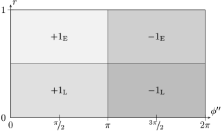
FIG. 3.: The measurement result at the right station given by the shifted hidden variables. The symbols have the same meaning as in Fig. 2.

At the right detector station, a similar procedure is followed. The result now depends on $(\phi,r)$ and the local setting $\phi_{2}$ of the apparatus. In this case, the shift is to the value $\phi^{\prime\prime}=\phi+\phi_{2}$, and the result is obtained in Fig. 3 in the same manner as before [15].

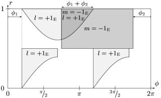
FIG. 4.: The shaded regions give the values for the initial hidden variables for which $l=+1_{\text{E}}$ or $m=-1_{\text{E}}$ are obtained (note that $\phi^{\prime}=\phi-\phi_{1}$ while $\phi^{\prime\prime}=\phi+\phi_{2}$). The overlap region of length $\phi_{1}+\phi_{2}$ represents the hidden variables for which both $l=+1_{\text{E}}$ and $m=-1_{\text{E}}$ are obtained.

The single-particle detection probabilities follow the quantum predictions as given by (6). The coincidence probabilities are determined by interposing Fig. 2 and Fig. 3 with the proper shifts. The probability of having $l=+1_{\text{E}}$ and $m=-1_{\text{E}}$ simultaneously is the area of the set indicated in Fig. 4 divided by $2\pi$ (the total area is $2\pi$ whereas the total probability is 1). The probability of the result $(+1,\text{E};-1,\text{E})$ is easily obtained, and because of the symmetry of the model, the probability of $(+1,\text{L};-1,\text{L})$ is the same. Since it is not possible to distinguish these two results from each other, the probability of interest is

$$P\bigl{(}+1;-1(\text{coincidence})|\phi_{1},\phi_{2}\bigr{)}$$ (7)

$$\qquad=P(+1,\text{E};-1,\text{E}|\phi_{1},\phi_{2})$$ (8)

$$\qquad\qquad+P(+1,\text{L};-1,\text{L}|\phi_{1},\phi_{2})$$ (9)

$$\qquad=\frac{2}{2\pi}\int_{0}^{\phi_{1}+\phi_{2}}\frac{\pi}{8}\sin(\phi)d\phi$$ (10)

$$\qquad=\frac{1}{8}\bigl{(}1-\cos{(\phi_{1}+\phi_{2})}\bigr{)},$$ (11)

which is equal to the quantum prediction. The other probabilities of simultaneous detection are obtained in the same manner. The probabilities for non-simultaneous detection are also obtained by integration, but here the symmetry of the model is such that e.g.

$$P(+1,\text{E};-1,\text{L}|\phi_{1},\phi_{2})$$ (12)

$$\qquad=\frac{1}{2\pi}\int_{0}^{\pi/2}\bigl{(}\frac{1}{2}-\frac{\pi}{8}\sin(\phi)\bigr{)}d\phi=\frac{1}{16},$$ (13)

independently of the detector settings, also in accordance with the quantum predictions. Finally, if the emission time on one side is monitored (by removing the interferometer), the counts on the other side still must follow the same local model, and as it is evident from the figures 1 and 2 the counts split evenly between early and late ones.

Let us now move into the conclusions. As the coincident events constitute only $50\%$ of all events, one might want to dismiss the whole problem by stating that effectively only around $\sqrt{50\%}\approx 71\%$ events at a single detection station enter into the Bell analysis, which is much below the usual threshold of minimum $83\%$ [16]. However, this is also the case in many other interferometric Bell-type configurations, e.g. [8], but performing a careful analysis it is still possible to show unconditional violations of local realism for the quantum predictions describing the expected phenomena in the ideal case [9]. The above construction shows that it is not possible to extend this analysis to Franson-type experiments.

The main conclusion of our work is that all experiments with Franson-type two-particle interferometers have to be reinterpreted. They cannot ever serve as demonstrations of violation of local realism (or, if preferred, violation of a Bell inequality), simply because there exists a LHV model for the expected quantum predictions in the ideal case. We emphasize that this model does not rely on any imperfections of the actual experiments (like the notorious detector-efficiency loophole).

One should notice here that majority of the performed quantum cryptography experiments that involve entanglement are based on the Franson two-particle interferometry. The original idea of harnessing quantum entanglement to cryptographic jobs was based on the fact that security checks can always be performed by testing whether the signals violate the Bell inequalities [17]. We have shown that such violations are only apparent for the studied Franson-type processes. Therefore, the basis for the application of this type of phenomena for quantum cryptography has to be carefully re-examined (compare [18]).

Facing our result, one could say that currently only the polarization entanglement setups are capable to produce true long-distance EPR-Bell type phenomena. Nevertheless, the Franson two-particle interferometry remains one of the most beautiful ways to demonstrate the non-classical nature of light (as the phenomena cannot be described by any classical field theory). Our ad hoc model is important only in relation to the Bell theorem.

Sven Aerts and Marek Żukowski were supported by the Flemish-Polish Scientific Collaboration Program No. 007. Marek Żukowski acknowledges support of UG Program BW/5400-5-0202-8. Sven Aerts is supported by the Flemish Institute for the advancement of Scientific-Technological Research in the Industry (IWT). Jan-Åke Larsson acknowledges support from the Swedish Natural Science Research Council.

REFERENCES

- [1] Electronic address: jalar@mai.liu.se
- [2] Electronic address: saerts@vub.ac.be
- [3] Electronic address: fizmz@univ.gda.pl
- [4] J. D. Franson, Phys. Rev. Lett. 62, 2205 (1989). We are not interested here in modifications of Franson’s idea like those in P. G. Kwiat, Phys. Rev. A 52, 3380 (1995) or D.V. Strekalov, T.B. Pittman, A.V. Sergienko, Y.H. Shih and P.G. Kwiat, Phys. Rev. A 54, R1 (1996), which in addition use initial polarization entanglement.
- [5] P. G. Kwiat, W. A. Vareka, C. K. Hong, H. Nathel and R. Y. Chiao, Phys. Rev. A 41, 2910 (1990); Z. Y. Ou, X. Y. Zou, L. J. Wang and L. Mandel, Phys. Rev. Lett. 65, 321 (1990). In these experiments the time resolution was not sharp enough to distinguish between the exactly coincident events and those differing in time by . The first experiment with high resolution is by J. Brendel, E. Mohler and W. Martiensen, Phys. Rev. Lett. 66, 1142 (1991), however their arrangement still involved Michelson interferometers. The first full realization of the Franson idea seems to be in P. G. Kwiat, A. M. Steinberg and R. Y. Chiao, Phys. Rev. A 47, R2472 (1993). For cryptographic applications see e.g. P. R. Tapster, J. G. Rarity, and P. C. M. Owens, Phys. Rev. Lett., 73, 1923 (1994), or very recently W. Tittel, J. Brendel, H. Zbinden, and N. Gisin, Phys. Rev. Lett. 81, 3563 (1998).
- [6] J. D. Franson, Phys. Rev. Lett. 67, 290 (1991); Z. Y. Ou and L. Mandel, J. Opt. Soc. Am. B 7, 2127 (1990).
- [7] A typical discussion of the role of the discarded events in the tests of local realism can be found in P. G. Kwiat, P. H. Eberhard, A. M. Steinberg and R. Y. Ciao, Phys. Rev. A 49, 3209 (1994).
- [8] Z. Y. Ou and L. Mandel, Phys. Rev. Lett. 61, 50 (1988); Y. H. Shih and C. O. Alley, Phys. Rev. Lett. 61 2921 (1988). Noncollinear correlated pairs of photons were entering opposite sides of a 50–50 beamsplitter. The photons entering one port were horizontally polarized, while those entering the other port were polarized vertically. Coincidence rates between detectors observing the two output ports were measured as a function of the orientations of the polarizers in front of them. Events where the two photons both exit via the same port were discarded from the analysis. In this way, exactly like in the case of Franson interferometry, of the initial ensemble was postselected.
- [9] S. Popescu, L. Hardy and M. Żukowski, Phys. Rev. A., 56, R4353 (1997).
- [10] The model of E. Santos, Phys. Lett. A, 212, 10 (1996) for the Franson type experiment is limited to detection efficiency lower than , and therefore it cannot describe the quantum mechanical predictions for the ideal case.
- [11] In the paper of L. De Caro and A. Garuccio, Phys. Rev. A 50, R2803 (1994) it is shown that certain Bell inequalities are not violated in the case of experiments [8], and in the discussion the authors mention that their results “can be easily extended” to the case of the Franson interferometry. However, in [9] it is shown that the experiments [8] violate Bell inequalities of a different type than the one studied by De Caro and Garuccio.
- [12] Some of the laboratory realizations of the experiment used two Michelson interferometers. However, such devices, due to the inherent loss of counts preclude any link of Franson type interferometry with Bell’s theorem. The generic setup for Franson type interferometry must involve Mach-Zehnder interferometers.
- [13] C. K. Hong and L. Mandel, Phys. Rev. A 31 2409 (1985); S. Friberg, C. K. Hong and L. Mandel, Phys. Rev. Lett. 54, 2011 (1985); P. G. Kwiat, A. M. Steinberg and R. Y. Chiao, Phys. Rev. A 45, 7729 (1992).
- [14] This is warranted by the spontaneous nature of the PDC emissions, and the continuity of the laser pump field. An interesting feature of the Franson-type interferometry is that the PDC source cannot be of pulsed nature (more precisely if the source is pulsed, the temporal width of the pulse cannot be shorter than ). If there is an unambiguous information about the emission time, the two-photon interference cannot occur. Simply, comparison of the detection time and the emission time reveals the path taken by the particle.
- [15] In the form presented here the model is asymmetric, but it may be trivially symmetrized.
- [16] J. F. Clauser and A. Shimony, Rep. Prog. Phys., 41, 1881 (1978); A. Garg and N. D. Mermin, Phys. Rev. D, 35, 3831 (1987); J.-Å. Larsson, Phys. Rev. A, 57 3304 (1998).
- [17] A. K. Ekert (1991), Phys. Rev. Lett., 67, 661.
- [18] M. Czachor (preprint, quant-ph/9812029).