Single-Step Quantum Search Using Problem Structure

Abstract

The structure of satisfiability problems is used to improve search algorithms for quantum computers and reduce their required coherence times by using only a single coherent evaluation of problem properties. The structure of random k-SAT allows determining the asymptotic average behavior of these algorithms, showing they improve on quantum algorithms, such as amplitude amplification, that ignore detailed problem structure but remain exponential for hard problem instances. Compared to good classical methods, the algorithm performs better, on average, for weakly and highly constrained problems but worse for hard cases. The analytic techniques introduced here also apply to other quantum algorithms, supplementing the limited evaluation possible with classical simulations and showing how quantum computing can use ensemble properties of NP search problems.

1 Introduction

Quantum computers [3, 5, 17, 18, 19, 20, 39, 43] offer the possibility of faster combinatorial search by operating simultaneously on all search states. For instance, quantum computers can factor integers in polynomial time [47], a problem thought to be intractable for classical machines.

At first sight, quantum computers seem particularly well-suited for NP search problems [22] due to their efficiently-computable test of whether a given search state is a solution. Quantum computers can apply this test to exponentially many search states in about the same time as a conventional (“classical”) computer tests just one and a variety of search algorithms have been proposed [8, 9, 10, 11, 27, 26, 30, 49]. However, extracting a definite answer from this simultaneous evaluation appears to still give an exponentially growing search cost in the worst case [4].

For general NP searches, amplitude amplification [27], using a test of whether a search state is a solution, quadratically improves performance of heuristics consisting of many independent trials [9]. This is the best possible improvement for “unstructured” quantum methods, i.e., those using only such a test [4]. Moreover, this technique does not apply to more complex heuristics, e.g., those involving backtracking, tabu lists, parameters adjusted based on unsuccessful trials, cached nogoods or other forms of learning, abstraction or extensive preprocessing. Such heuristics often provide the best known performance, at least on average, for a variety of combinatorial searches. A focus on typical behavior of large problems is important because often the worst cases are far harder than most instances encountered in practice.

Thus, as a practical matter, there remain the questions of whether using problem structure in quantum algorithms can give more than quadratic improvement for the heuristics consisting of independent trials, any improvement at all for other types of heuristics, and less than exponential cost for at least some typical problems arising in practice. As one example, further improvement is possible for a quantum algorithm using detailed information on the distance of search states to solutions [28], but in practice, such information is not readily available for most searches.

Addressing these questions requires developing algorithms using problem structure and determining their behavior for large problems. As with classical heuristics, such algorithms are often difficult to analyze theoretically due to complicated dependencies among successive search choices. Thus one is often forced to use empirical evaluation with a sample of problems. While quite common for evaluating classical heuristics, this approach is limited to small problems for quantum algorithms on current machines due to the exponential increase in time and memory required for the classical simulation. Another approach, applied in this paper, evaluates average behavior over a simple ensemble of problems. Such ensemble-based analyses provide insight into typical behavior for large problems [51].

An extreme case is single-step quantum search, i.e., algorithms using only a single evaluation of structure associated with a problem. Single-step search is very effective for highly constrained problems [31], outperforming both unstructured quantum search and classical heuristics in these cases. Can the technique used for highly constrained problems be extended to the more challenging case of hard search problems with an intermediate number of constraints [12, 33]? Conversely, to what extent does the restriction to a single step limit the extent to which the capabilities of quantum computers can be used?

Single-step search is particularly well-suited for an ensemble-based analysis, since it avoids the dependencies found in multistep quantum algorithms or classical heuristics. Furthermore, single-step methods require far less coherence time than the unstructured algorithm with its exponentially many steps, and hence should be easier to implement. This is because maintaining coherence over many computational steps is difficult [38, 50, 29, 40]. While this difficulty is unlikely to be a fundamental limitation [6, 46, 37] and small quantum computations have been implemented [14, 13], algorithms that minimize the required coherence time simplify hardware implementation.

This paper gives an ensemble analysis for a single-step algorithm using the number of conflicts in each search state. We evaluate the asymptotic average scaling behavior directly, rather than relying on simulations. This result allows optimizing the algorithm, and also demonstrates a general technique for studying the average behavior of quantum search algorithms. We compare the asymptotic predictions to evaluations of small cases accessible to simulation, showing good correspondence even for small problems.

In the remainder of this paper, we first summarize the NP-complete satisfiability search problem and then describe a class of one-step quantum algorithms for it. This class includes both the previous unstructured and highly constrained methods as special cases. We identify the best performing algorithms for satisfiability problems with differing degrees of constraint in the following two sections. We then present some additional behaviors of the algorithm and briefly consider extensions to more complex algorithms suggested by these results. Details of the derivation are in the appendices.

As a note on notation, to compare the growth rates of various functions we use [25] $f=O\left(g\right)$ to indicate that $f$ grows no faster than $g$ as a function of $n$ when $n\rightarrow\infty$. Conversely, $f=\Omega\left(g\right)$ means $f$ grows at least as fast as $g$, and $f=\Theta\left(g\right)$ means both functions grow at the same rate.

2 Satisfiability

Satisfiability (SAT) is a combinatorial search problem [22] consisting of a logical propositional formula in $n$ variables $V_{1},\ldots,V_{n}$ and the requirement to find a value (true or false) for each variable that makes the formula true. This problem has $N=2^{n}$ assignments. For $k$-SAT, the formula consists of a conjunction of clauses and each clause is a disjunction of $k$ variables, any of which may be negated. For $k\geq 3$ these problems are NP-complete. A clause with $k$ variables is false for exactly one assignment to those variables, and true for the other $2^{k}-1$ choices. An example of such a clause for $k=3$, with the third variable negated, is $V_{1}$ OR $V_{2}$ OR (NOT $V_{3}$), which is false for $\{V_{1}=\mbox{\sc false},V_{2}=\mbox{\sc false},V_{3}=\mbox{\sc true}\}$. Since the formula is a conjunction of clauses, a solution must satisfy every clause. We say an assignment conflicts with a clause when the values the assignment gives to the variables in the clause make the clause false. For example, in a four variable problem, the assignment

$$\{V_{1}=\mbox{\sc false},V_{2}=\mbox{\sc false},V_{3}=\mbox{\sc true},V_{4}=\mbox{\sc true}\}$$

conflicts with the $k=3$ clause given above, while

$$\{V_{1}=\mbox{\sc false},V_{2}=\mbox{\sc false},V_{3}=\mbox{\sc false},V_{4}=\mbox{\sc true}\}$$

does not. Thus each clause is a constraint that adds one conflict to all assignments that conflict with it. The number of distinct clauses $m$ is then the number of constraints in the problem.

The assignments for SAT can also be viewed as bit-strings with the correspondence that the $i^{th}$ bit is 0 or 1 according to whether $V_{i}$ is assigned the value false or true, respectively. In turn, these bit-strings are the binary representation of integers, ranging from 0 to $2^{n}-1$. For definiteness, we arbitrarily order the bits so the values of $V_{1}$ and $V_{n}$ correspond, respectively, to the least and most significant bits of the integer. For example, the assignment

$$\{V_{1}=\mbox{\sc false},V_{2}=\mbox{\sc false},V_{3}=\mbox{\sc true},V_{4}=\mbox{\sc false}\}$$

corresponds to the integer whose binary representation is 0100, i.e., the number 4.

For bit-strings $r$ and $s$, let ${|s|}$ be the number of 1-bits in $s$ and $r\wedge s$ the bitwise AND operation on $r$ and $s$. Thus ${|r\wedge s|}$ counts the number of 1-bits both assignments have in common. We also use $d(r,s)$ as the Hamming distance between $r$ and $s$, i.e., the number of positions at which they have different values. These quantities are related by

$$d(r,s)={|r|}+{|s|}-2{|r\wedge s|}$$ (1)

Let $c(s)$ be the number of conflicts for assignment $s$ in a given SAT problem.

An example 1-SAT problem with $n=2$ is the propositional formula (NOT $V_{1}$) AND (NOT $V_{2}$). This problem has a unique solution: $\{V_{1}=\mbox{\sc false},V_{2}=\mbox{\sc false}\}$, an assignment with the bit representation 00. The remaining assignments for this problem have bit representations 01, 10, and 11.

Theoretically, search algorithms are often evaluated for the worst possible case. However, in practice, search problems are often found to be considerably easier than suggested by these worst case analyses [33]. This observation leads to examining the typical behavior of search algorithms with respect to a specified ensemble of problems, i.e., a class of problems and a probability for each to occur. A useful ensemble is random $k$-SAT, specified by the number of variables $n$, the size of the clauses $k$ and the number of distinct clauses $m$. A problem instance is created by randomly selecting $m$ distinct clauses from the set of all possible clauses [41]. When $n$ is large, the typical behavior of random $k$-SAT is determined by $\mu=m/n$, the ratio of clauses to variables. In particular, for each $k$ there is a threshold value ${\mu_{\rm crit}}$ on $\mu$ below which most random $k$-SAT problems are soluble and above which most have no solutions [15, 44]. For $k=3$, this value is approximately ${\mu_{\rm crit}}=4.2$.

The quantum searches considered here are incomplete methods, i.e., they can find a solution if one exists but can never guarantee no solution exists. For studying such algorithms, the ensembles would ideally contain only instances with a solution. For example, we could consider the ensemble of random soluble $k$-SAT, in which each instance with at least one solution is equally likely to appear. Unfortunately, this ensemble does not have a simple expression for the number of problems as required for the analytic performance evaluation given below. Instead, for $\mu<{\mu_{\rm crit}}$, most random problems indeed have a solution so random $k$-SAT is useful for studying incomplete search methods for underconstrained problems.

Randomly selected overconstrained problems usually have no solutions so random SAT is not a useful ensemble when $\mu>{\mu_{\rm crit}}$. An alternative with simple analytic properties is the ensemble with a prespecified solution. In this case, a particular assignment is selected to be a solution. Then the $m$ clauses are selected from among those that do not conflict with the prespecified solution. Compared to random selection among soluble problems, using a prespecified solution is more likely to pick problems with many solutions, resulting in somewhat easier search problems, on average.

Each clause in a $k$-SAT formula conflicts with exactly one of the $2^{k}$ possible assignments for the variables that appear in the clause. Thus the average number of conflicts in an assignment is ${c_{\rm avg}}=m/2^{k}$. While this average is the same for all SAT problems with given $m$ and $k$, the variance in the number of conflicts varies from problem to problem. As described in Appendix A, the the variance for random $k$-SAT is ${c_{\rm avg}}(1-2^{-k})$. Thus when $m\gg 1$, the relative deviation decreases as $O\left(1/\sqrt{m}\right)$ and hence the number of conflicts in most assignments is very close to the average.

For random $k$-SAT, the expected number of solutions is [51]

$$\left\langle S\right\rangle=2^{n}(1-2^{-k})^{m}=2^{n}\exp(\mu n\log(1-2^{-k}))$$ (2)

3 Quantum Search Algorithms

Quantum computers use physical devices whose full quantum state can be controlled. For example [19], an atom in its ground state could represent a bit set to 0, and an excited state for 1. The atom can be switched between these states and also be placed in a uniquely quantum mechanical superposition of these values, which can be denoted as a vector $\pmatrix{\psi_{0}\cr\psi_{1}\cr}$, with a component (called an amplitude) for each of the corresponding classical states for the system. These amplitudes are complex numbers.

A quantum machine with $n$ quantum bits exists in a superposition of the $2^{n}$ classical states for $n$ bits. The amplitudes have a physical interpretation: when the computer’s state is measured, the superposition randomly changes to one of the classical states with $|\psi_{s}|^{2}$ being the probability to obtain the state $s$. Thus amplitudes satisfy the normalization condition $\sum_{s}|\psi_{s}|^{2}=1$. This measurement operation is used to obtain definite results from a quantum computation.

Quantum algorithms manipulate the amplitudes in a superposition. Because quantum mechanics is linear and the normalization condition must always be satisfied, these operations are limited to unitary linear operators. That is, a state vector $\psi$ can only change to a new vector $\psi^{\prime}$ related to the original one by a unitary transformation, i.e., $\psi^{\prime}=U\psi$ where $U$ is a unitary matrix of dimension $2^{n}\times 2^{n}$. In spite of the exponential size of the matrix, in many cases the operation can be performed in a time that grows only as a polynomial in $n$ by quantum computers [8, 35, 34]. Importantly, the quantum computer does not explicitly form, or store, the matrix $U$. Rather it performs a series of elementary operations whose net effect is to produce the new state vector $\psi^{\prime}$. The components of the new vector are not directly accessible: rather they determine the probabilities of obtaining various results when the state is measured.

Search algorithms for SAT problems use efficiently computed properties of individual assignments, e.g., a test of whether a given assignment is a solution. With quantum computers, these properties can be evaluated simultaneously for all assignments. In this paper we focus on algorithms that make use of this simultaneous evaluation just once.

3.1 Single-Step Search

Single-step methods could be implemented in a variety of ways. One simple approach starts with an equal superposition of all the assignments, adjusts the phases based on the number of conflicts in each of the assignments, and then mixes the amplitudes from different assignments. This algorithm requires only a single testing of the assignments, corresponding to a single classical search step.

For a $k$-SAT problem with $n$ variables and $m$ clauses, the algorithm takes the following form. The initial state has amplitude $\psi_{s}=2^{-n/2}$ for each of the $2^{n}$ assignments $s$, and the final state vector is $\phi=UP\psi$ where the matrices $P$ and $U$ are defined as follows. The matrix $P$ is diagonal with $P_{ss}=p_{c(s)}$ depending on the number of conflicts $c$ in the assignment $s$, ranging from 0 to $m$. Because the number of conflicts in a given assignment is efficiently computable for SAT problems, these phase choices can be efficiently implemented [34].

The mixing matrix is defined in terms of two simpler operations: $U=WTW$. The Walsh transform $W$ has entries

$$W_{rs}=2^{-n/2}(-1)^{|r\wedge s|}$$ (3)

for assignments $r$ and $s$ and can be implemented efficiently [8, 27]. The matrix $T$ is diagonal with elements $T_{rr}=t_{{|r|}}$ depending only on the number of 1-bits in each assignment, ranging from 0 to $n$. These definitions for $W$ and $T$ lead to a mixing matrix $U$ whose elements $U_{rs}=u_{d(r,s)}$ depend only on the Hamming distance between the assignments $r$ and $s$, with [32]

$$u_{d}=2^{-n}\sum_{z=0}^{d}\sum_{h=z}^{n-d+z}(-1)^{z}{d\choose z}{n-d\choose h-z}t_{h}$$ (4)

Unlike previous algorithms, where phase choices are often just $\pm 1$, this algorithm potentially uses a different phase choice for each number of conflicts and each number of 1-bits in an assignment.

This procedure defines a class of algorithms. A particular choice of the phases $p_{c}$ and $t_{h}$ completes the algorithm’s specification. For example, the choices $p_{0}=1$, $t_{0}=1$ and the remaining phases set to $-1$ gives a single step of the unstructured search algorithm [27]. Another example is $p_{c}=i^{c}$ and $t_{h}=i^{h}$, appropriate for maximally constrained 1-SAT problems [31].

3.2 Selecting Phase Values

To determine appropriate choices for $p_{c}$ and $t_{h}$, we can evaluate the algorithm, via classical simulation, for samples of random SAT problems with small $n$ using a variety of choices for $p_{c}$ and $t_{h}$. Numerical optimization of average performance with respect to these choices then identifies values giving high performance for random $k$-SAT. These optimal values show $\log p_{c}$ and $\log t_{h}$ vary nearly linearly with $c$ and $h$ over most of their range. This observation suggests that restricting consideration to such linear variation is likely to give a reasonable idea of the best such algorithms can perform, while simplifying the analysis.

To further understand why such choices are appropriate for large $k$-SAT problems, note that the number of assignments with $h$ 1-bits is $n\choose h$. So for large $n$, most have $h$ close to $n/2$. Similarly, for the phases $p_{c}$, provided the number of clauses is large, i.e., $m\gg 1$, most assignments have nearly the average number of conflicts ${c_{\rm avg}}=m/2^{k}$. For large problems, we can expect the behavior of the phases near the average values will be the only important choices influencing the algorithm’s behavior. Thus we consider an expansion around the dominant values of the form

$$t_{h}=\exp\left(i\pi\left(\tau^{(0)}+\tau^{(1)}\left(h-\frac{n}{2}\right)+\tau^{(2)}\left(h-\frac{n}{2}\right)^{2}+\ldots\right)\right)$$ (5)

where the $\tau^{(i)}$ are constants, and similarly for $p_{c}$. The first term in such an expansion just gives a constant overall phase factor for the amplitudes, which has no effect on the probability to find a solution, and so can arbitrarily be set equal to zero. The next term in the expansion, giving linear variation in phases, affects the solution probability. For assignments close to the average, this linear variation dominates the behavior.

From both the empirical observations on optimal phase values for small problems and the increasing concentration of values for $h$ and $c$ and $n$ increases, we are led to consider a linear variation in the phase values. If, in spite of these motivating arguments, including some nonlinearity in the phase values improves the leading asymptotic behavior, a restriction to linear variation would still provide a lower bound on the possible performance of single-step algorithms. Thus we restrict consideration to phase choices described by two constants $\rho$ and $\tau$ with

$$p_{c}=e^{i\pi\rho(c-{c_{\rm avg}})}$$ (6)

and

$$t_{h}=e^{i\pi\tau(h-n/2)}$$ (7)

The terms ${c_{\rm avg}}$ and $n/2$ in these expressions just give an irrelevant overall phase to the amplitudes, but slightly simplify the analysis. As shown in Appendix B this choice for $t_{h}$ gives

$$u_{d}=\cos^{n}\left(\frac{\pi\tau}{2}\right)\tan^{d}\left(\frac{\pi\tau}{2}\right)(-i)^{d}$$ (8)

For example, when $\tau=1/2$, $u_{d}=2^{-n/2}(-i)^{d}$ as used for solving 1-SAT problems [31].

Because $c$ and $h$ are integers, it is sufficient to consider values for $\rho$ and $\tau$ in the range $-1$ to 1. Since changing the sign of both $\rho$ and $\tau$ simply conjugates the amplitudes, we can further restrict consideration to $\tau$ in the range 0 to 1.

Completing the algorithm requires particular choices for $\rho$ and $\tau$. The asymptotic analysis given below identifies optimal choices for these parameters based on the values of $k$ and $m/n$.

3.3 Asymptotic Behavior for Random $k$-SAT

When the phase choices are particularly simple, as with the unstructured search algorithm [27], or the problem has a simple relation between Hamming distance from a solution and number of conflicts, as in 1-SAT problems [31], the probability to obtain a solution, $P_{\rm soln}$, has a simple analytic form. In more general cases, the solution probability can only be evaluated with a classical simulation, limiting the study of more complex algorithms or problem structures to relatively small sizes. A third approach to evaluating $P_{\rm soln}$ is to average over an ensemble of problems. This approach, developed in Appendix C, uses the structure of search problem ensembles to analyze the asymptotic behavior of the algorithm, and hence to select the best values for $\rho$ and $\tau$. Specifically, for random $k$-SAT, the average of $P_{\rm soln}$ scales as

$$\left\langle P_{\rm soln}\right\rangle\propto e^{-nA(k,\mu,\rho,\tau)}$$ (9)

where the decay rate $A$ can be evaluated numerically for given choices of $k$, $\mu$, $\rho$ and $\tau$.

Given the ability to numerically compute $A$, we can then optimize the performance of the algorithm, measured in terms of the average probability to find a solution, i.e., minimizing $A$. This numerical optimization gives values for $\rho$ and $\tau$ appropriate to random $k$-SAT with a given value of $\mu$.

In practice, implementation limitations will introduce some errors in the parameters. Fortunately, the precision required is not particularly strict because the parameters appear in the exponents. In particular, an error of $\epsilon$ in $\rho$ or $\tau$ will give error $O\left(\epsilon^{2}\right)$ in the exponent. Thus only a square root precision in the implementation of the values of $\rho$ and $\tau$ is required. While by no means trivial, this shows the algorithm does not require exponentially precise parameter values to achieve the scaling.

As an example, for the weakly constrained case in §5, such errors in parameter values gives exponential decay of $\exp(O\left(\epsilon^{2}\right)m)$. To maintain $\Theta\left(1\right)$ behavior, $\epsilon$ must be small enough that $\epsilon^{2}m=\Theta\left(1\right)$, i.e., the precision requirement is $\epsilon=O\left(1/\sqrt{m}\right)$. The precise scaling due to errors depends on the size of the second derivatives of $A$ around the optimal $\rho$ and $\tau$ values. For $k=3$, a root-mean-square combined error of $\epsilon$ in $\rho$ and $\tau$ introduces at worst a factor $\exp(-3.18\epsilon^{2}m)$. This is greater than 1/2 provided $\epsilon<0.46/\sqrt{m}$. For example, weakly constrained problems with $m=2\sqrt{n}$ satisfy this requirement for a 10,000 variable problem provided $\epsilon<0.033$, which allows, roughly, a 10% error in the parameter values. Similarly, for $m\gg n$, such parameter errors give exponential decay of $\exp(O\left(\epsilon^{2}\right)n)$, so the precision requirement is $\epsilon=O\left(1/\sqrt{n}\right)$.

3.4 Unstructured Search

As a point of comparison with the one-step algorithm based on the number of conflicts in assignments, the unstructured search algorithm [27] applies amplitude amplification to random selection, giving a quadratic speedup after an exponentially large number of steps. Specifically, for a problem with $n$ variables and $S$ solutions, the probability in solutions after $j$ steps is [8] $\sin^{2}((2j+1)\theta)$ with $\sin(\theta)=\sqrt{S/2^{n}}$.

From Eq. (2), for random $k$-SAT with fixed $\mu$ the fraction of assignments that are solutions, $S/2^{n}$, is exponentially small, and $\theta\approx e^{\mu n\log(1-2^{-k})/2}$. Thus for any fixed number of steps, $j$, the scaling of $\left\langle P_{\rm soln}\right\rangle$ is $\Theta\left(e^{\mu n\log(1-2^{-k})}\right)$, the same as random selection. This scaling is independent of the number of steps (provided $j$ is constant). When $j$ increases exponentially with $n$, specifically $j=\Theta\left(\theta^{-1}\right)$, then the probability of a solution with this unstructured algorithm is $\Theta\left(1\right)$.

More generally, given a classical or quantum method consisting of independent trials, each of which produces a solution with probability $p$, amplitude amplification produces the quadratic improvement [9] with $\sin(\theta)=\sqrt{p}$. Thus the cost is $\Theta\left(1/\sqrt{p}\right)$ times the cost for a single trial. This general result means quantum computers can improve on many classical methods. However this quadratic improvement is also the best possible for quantum methods based only on testing whether assignments are solutions [4]. Moreover, some classical heuristics use information from unsuccessful trials to improve future ones, i.e., trials are not independent. Others spend most of their effort in preprocessing followed by rapid identification of the solution. In these cases, even this quadratic improvement does not apply.

4 Solving Hard Problems

For random $k$-SAT, the hardest problem instances are concentrated near a threshold value of $\mu=m/n$ depending on $k$. For 3-SAT, this threshold is at $\mu=4.2$ [15]. Thus we examine the behavior of the single step algorithm when $\mu$ is constant. In this case, the minimum decay rate $A$ is shown in Fig. 1. The corresponding best choices for $\rho$ and $\tau$ are shown in Fig. 2. Note that the $\tau$ values are less than 1/2 which, from Eq. (8), means the $u_{d}$ matrix elements are largest for small $d$, hence emphasizing the mixing at distances less than $n/2$ allowing the algorithm to exploit the clustering of assignments with relatively few conflicts in $k$-SAT. These values, obtained by numerical minimization of $A$ with respect to $\rho$ and $\tau$, could be local minima. If so, other choices for $\rho$ and $\tau$ would give even better performance than the values reported here. For comparison, Fig. 1 shows the scaling of random selection, $\left\langle S\right\rangle/2^{n}$, where $S$ is the number of solutions, using Eq. (2).

Figure 1: Smallest exponential decay rate $A$ for $\left\langle P_{\rm soln}\right\rangle$ as a function of $\mu=m/n$ for random 3-SAT. For comparison, the gray curve shows the scaling for random selection. The points indicate empirical estimates of the decay rate for the fraction of soluble problems, a lower bound on the decay rate for $P_{\rm soln}$. For large $\mu$, these estimates are difficult to obtain. A weaker lower bound, shown as the upper edge of the filled region, is given by the Markov bound using expected number of solutions for random 3-SAT.

	random			prespecified
$\mu$	$\tau$	$\rho$	$A$	$\tau$	$\rho$	$A$
1	0.238	0.348	$0.027$	0.239	0.344	$0.026$
2	0.260	0.291	$0.094$	0.262	0.286	$0.088$
3	0.275	0.249	$0.181$	0.278	0.242	$0.162$
4	0.286	0.218	$0.280$	0.293	0.211	$0.231$
5	0.295	0.195	$0.386$	0.304	0.188	$0.281$
6	0.303	0.176	$0.497$	0.311	0.172	$0.309$

Table 1: Best parameter values and scaling behavior for single-step search of 3-SAT problems for random and prespecified solution ensembles.

Figure 2: Optimal choices of $\tau$ (black) and $\rho$ (gray) as a function of $\mu=m/n$. Solid curves are for the random 3-SAT ensemble and the dashed curves are for the ensemble with a prespecified solution.

An important observation from these results is even the best use of problem structure based only on the number of conflicts cannot remove the exponential search cost with a single step algorithm of the type described here.

The unstructured search algorithm [27] consists of applying amplitude amplification to random selection. Thus a second observation from Fig. 1 is, for $\mu$ less than about 3.5 (where $A<-\frac{1}{2n}\log(\left\langle S\right\rangle/2^{n})$), a single step with the optimal choices of $\rho$ and $\tau$ gives exponentially better performance, on average, than the unstructured search algorithm, which also requires coherence extending over multiple steps. Thus this analysis demonstrates how the structure of search ensembles can be exploited to improve quantum search performance and simultaneously reduce the required coherence time. Moreover, by giving the actual asymptotic scaling this result is more definitive than prior empirical studies of algorithms based on classical simulations of small problems [30].

Furthermore, the one-step algorithm can be combined with amplitude amplification [9] to achieve an additional quadratic improvement, corresponding to dividing the decay rate by a factor of 2 for soluble problems. This combination requires extending coherence time beyond just one step, but because the reduced decay rate is then below that of the unstructured algorithm over the whole range of $\mu$, not only is performance better but the coherence time is still less than that of the unstructured algorithm. Thus this new algorithm improves on the unstructured one, on average, over the whole range of $\mu$.

As another comparison, the cost of a good classical heuristic method is empirically observed [15] to scale as $2^{n/19.5}$ for random 3-SAT problems near $\mu=4.2$, corresponding to $A$ equal to $\log(2)/19.5=0.036$. This scaling is better than the single-step quantum algorithm, which has $A=0.30$ for $\mu=4.2$. Even combined with amplitude amplification, reducing the decay rate to $0.15$, the classical heuristic remains better.

Beyond $\mu=4.2$, the fraction of soluble problems, ${P_{\rm soluble}}$, drops to zero as $n$ increases for random 3-SAT. The performance of this algorithm for soluble problems is given instead by $\left\langle P_{\rm soln}\right\rangle/{P_{\rm soluble}}$. Thus if ${P_{\rm soluble}}$ scales as $e^{-\omega n}$, the algorithm’s decay rate for random soluble problems is $A-\omega$, and $A$ is always at least as large as $\omega$. Unfortunately, the random $k$-SAT ensemble does not have a simple expression for ${P_{\rm soluble}}$, or even just its leading exponential scaling rate $\omega$, precluding an exact evaluation of the behavior with respect to overconstrained soluble problems.

One approach to estimate this behavior uses empirical classical search to evaluate ${P_{\rm soluble}}$ for a range of problem sizes for a given value of $\mu$. The behavior of these values as a function of $n$ then estimates $\omega$. For instance, a study [44] using samples of $10^{4}$ problems for $n$ from 50 to 250 shows close to exponential decrease of ${P_{\rm soluble}}$ for $\mu$ values somewhat above the transition. The resulting estimates of the actual decay rates for ${P_{\rm soluble}}$ are $0.011$, $0.025$ and $0.045$ for $\mu$ equal to $4.5$, $4.7$ and $4.9$, respectively. These values are considerably smaller than the value of $A$ for the one-step algorithm for these values of $\mu$, as shown in Fig. 1. Nevertheless, the increase in $\omega$ accounts for most of the increase in $A$ over this range of $\mu$ values, i.e., the soluble problems are not continuing to get much harder for this one-step algorithm above the transition.

This empirical technique is increasingly difficult to apply as $\mu$ increases due to the rapidly decreasing fraction of soluble problems in the ensemble [44]. For larger $\mu$ we can instead obtain a lower bound on the decay rate for ${P_{\rm soluble}}$ using the Markov inequality: ${P_{\rm soluble}}\leq\left\langle S\right\rangle$. That is, this analysis averages over all problems in the ensemble, so $\left\langle P_{\rm soln}\right\rangle\leq{P_{\rm soluble}}$. Thus, $\left\langle P_{\rm soln}\right\rangle\leq{P_{\rm soluble}}\leq\left\langle S\right\rangle$, corresponding to $A\geq\omega\geq-\frac{1}{n}\log\left\langle S\right\rangle$. When $\mu>-\log(2)/\log(1-2^{-k})$ (equal to 5.19 for $k=3$), Eq. (2) gives $\left\langle S\right\rangle\rightarrow 0$ as $n\rightarrow\infty$ so this becomes a nontrivial bound as shown in Fig. 1. However, as a lower bound, this inequality cannot be used to determine whether overconstrained soluble problems indeed become easier to solve with the one-step algorithm as $\mu$ increases.

An alternate approach uses an ensemble where all problems are soluble and that is analytically simple, e.g., the ensemble with a prespecified solution described in §2. The evaluation of $\left\langle P_{\rm soln}\right\rangle$ proceeds as described in Appendix C, with the addition of needing to keep track of the distances of the assignments $r$, $s$ and $s^{\prime}$ to the prespecified solution (which affects the available number of clauses that can be selected to produce the required numbers of conflicts). The resulting optimal behavior is shown in Fig. 3, with the corresponding best values for $\rho$ and $\tau$ given in Fig. 2. The decay rate decreases as $\mu$ increases past 7, i.e., problems become easier as the number of clauses increases. Presumably a similar behavior would be seen for the soluble cases in the random ensemble as well because these two ensembles are fairly similar when $\mu$ is large. This observation of problems becoming easier as $\mu$ increases past the transtion corresponds to behavior seen with many classical methods. On the other hand, random selection and the unstructured algorithm do not improve as $\mu$ increases: they do not take advantage of the structure of highly constrained problems.

Figure 3: Smallest exponential decay rate $A$ for $\left\langle P_{\rm soln}\right\rangle$ as a function of $\mu=m/n$ for 3-SAT with prespecified solution. For comparison, the gray curve shows the scaling for random selection.

Since classical simulations of quantum algorithms are limited to few variables, this asymptotic analysis can also indicate the extent to which these simulations match the asymptotic behavior. An example is Fig. 4 showing that the behavior matches that from Table 1 for $\mu=2$ and $\mu=4$ even with a small number of variables. This suggests the limited sizes accessible with classical simulation may nevertheless be sufficient to indicate asymptotic behavior, as is also seen in some studies of classical heuristics [15].

Figure 4: Optimal asymptotic behavior of $\left\langle P_{\rm soln}\right\rangle$ for 3-SAT with $\mu=2$ (gray) and 4 (black) on a log-scale vs. $n$. The points show the exact values of $\left\langle P_{\rm soln}\right\rangle$.

5 Solving Weakly and Highly Constrained Problems

The behavior of the minimum decay rate shown in Fig. 1 and 3 suggests that $A$ decreases toward zero for small and large values of $\mu$ for soluble problems. This is confirmed in Fig. 5 which shows the behavior of both ensembles over a larger range of values.

As $\mu\rightarrow 0$, the figure shows the minimum decay rate is nearly a straight line with slope 2 on this log-log plot, indicating $A=\Theta\left(\mu^{2}\right)$ in this limit. With this limiting behavior $\left\langle P_{\rm soln}\right\rangle\propto e^{-An}$ with $An=\Theta\left(m^{2}/n\right)$. In particular, if $m$ grows no faster than $\sqrt{n}$, $\left\langle P_{\rm soln}\right\rangle$ will remain $\Theta\left(1\right)$ as $n$ increases.

Similarly, as $\mu\rightarrow\infty$, Fig. 5 shows $A$ decreasing in a straight line with slope $-1$, indicating $A=\Theta\left(1/\mu\right)$. Correspondingly, $An=\Theta\left(n^{2}/m\right)$. So if $m$ grows at least as fast as $n^{2}$, the probability to find a solution, on average, will remain $\Theta\left(1\right)$ as $n$ increases.

Figure 5: Limiting behaviors, on a log-log plot, for exponential decay rate $A$. Behavior for random 3-SAT (black curve, up to $\mu=6$), prespecified solution 3-SAT (gray curve, for $\mu$ between 0.1 and 40) and the upper bound based on probability to find the prespecified solution (black curve, for $\mu\geq 20$). For comparison the dashed lines show the limiting behaviors for small and large $\mu$, which correspond very closely to the exact values for $\mu<0.3$ and $\mu>1000$.

Appendix C confirms these observations. While such weakly and highly constrained problems are fairly easy, the single-step algorithm outperforms classical heuristic methods for these cases, which require evaluating $\Theta\left(n\right)$ assignments on average.

$n$	$m$	$\left\langle P_{\rm soln}\right\rangle$	$\left\langle S\right\rangle/2^{n}$
4	4	0.908	0.569
9	6	0.897	0.447
16	8	0.894	0.343
25	10	0.893	0.263
36	12	0.892	0.201

Table 2: Scaling of $\left\langle P_{\rm soln}\right\rangle$ from Eq. (23) and $\left\langle S\right\rangle/2^{n}$ for weakly constrained random 3-SAT with $m=2\sqrt{n}$.

As an example, when $k=3$, $A={\alpha_{\rm weak}}\mu^{2}$ with ${\alpha_{\rm weak}}=0.029405$, shown as the dashed line in Fig. 5 for the $\mu\rightarrow 0$ limit. For $\mu=2/\sqrt{n}$, Table 2 shows the approach to the asymptotic limit $e^{-An}=\exp(-4{\alpha_{\rm weak}})=0.889$. This behavior compares with the still rapid decrease in expected fraction of solutions which scales as $\left\langle S\right\rangle/2^{n}=(1-2^{-k})^{m}$ or $(7/8)^{m}$ for $k=3$. Thus the unstructured search scaling for this example is $(7/8)^{\sqrt{n}}$ which still decreases faster than polynomially.

At the other extreme, Appendix C.4 shows that as $\mu\rightarrow\infty$, $A\sim(2^{k}-1)^{3}\pi^{2}/(16k^{2}\mu)$, shown in Fig. 5. Hence, when $m=\Omega\left(n^{2}\right)$, we have $\Theta\left(1\right)$ performance. This analysis also improves on previous work based on a lower bound estimate [32] showing $\Theta\left(1\right)$ behavior for highly constrained problems, but only when $m$ grew faster than a particular multiple of $n^{2}$ (equal to 17.3 for $k=3$).

6 Problem Search Costs

The ensemble average leading to Eq. (9) provides a direct analysis of $\left\langle P_{\rm soln}\right\rangle$. This technique generalizes to quantities involving positive integer powers of $P_{\rm soln}$, such as the variance discussed in §7.1. Unfortunately the technique does not apply to quantities such as the expected solution cost which, for any particular problem, is $1/P_{\rm soln}$ for independent trials, or $\Theta\left(1/\sqrt{P_{\rm soln}}\right)$ when combined with amplitude amplification [9]. Thus an important question is the extent to which an analysis based on $\left\langle P_{\rm soln}\right\rangle$ provides insight into actual search costs, and hence is useful in selecting appropriate phase parameters.

We can approach this question through an empirical evaluation of a sample of problems. However, for characterizing the typical behavior of problems, it is important to keep in mind that ensembles with even one problem with no solutions have $\left\langle 1/P_{\rm soln}\right\rangle=\infty$. Even restricting consideration just to soluble problems, this ensemble average can be dominated by the exceptionally high costs of just a few instances, does not usefully characterize typical search behaviors. A more useful quantity is the median of $1/P_{\rm soln}$, whose properties are even more difficult to determine theoretically than the mean. Instead Table 3 compares these quantities based on classical simulation. We see that $\frac{1}{\left\langle P_{\rm soln}\right\rangle}$ underestimates the median search cost, but is a better estimate than $\left\langle 1/P_{\rm soln}\right\rangle$ even when restricted to soluble problems.

	$\mu=2$			$\mu=4$
$n$	$\frac{1}{\left\langle P_{\rm soln}\right\rangle}$	${\rm median}\left(\frac{1}{P_{\rm soln}}\right)$	$\left\langle\frac{1}{P_{\rm soln}}\right\rangle$	$\frac{1}{\left\langle P_{\rm soln}\right\rangle}$	${\rm median}\left(\frac{1}{P_{\rm soln}}\right)$	$\left\langle\frac{1}{P_{\rm soln}}\right\rangle$
10	2.6	2.6	2.8	15	17	25
20	6.6	6.8	7.4	228	352	705

Table 3: Comparison of search cost estimates based on 1000 soluble random 3-SAT problems using optimal parameter values from Table 1.

More generally we can examine the full distribution of problem search costs. For instance, Fig. 6 compares the unstructured method with the combination of amplitude amplification with the one-step algorithm. This shows a reduction in cost from using problem structure, corresponding with the above discussion of the relative costs, in conjunction with Fig. 1, based on the analysis of $\left\langle P_{\rm soln}\right\rangle$. The behavior of the unstructured search depends only on the number of solutions, leading to the vertical groups of points in the figure. By contrast, the structured method shows considerable variation in costs even among problems with the same number of solutions.

Figure 6: Comparison of search costs for the one-step quantum method combined with amplitude amplification and unstructured amplitude amplification. Each point shows the expected search cost for a single problem instance of random 3-SAT with $n=20$ and $m=80$, assuming the number of solutions and $P_{\rm soln}$ are known a priori. In practice these values will not be known a priori, increasing the costs by up to a factor of 4 [8].

The full distribution of costs available from empirical evaluation of a sample of random $k$-SAT problems can address questions beyond those possible by an analysis of average behavior. For example, to what extent do classical and quantum methods find the same problems particularly difficult? Fig. 7 compares the expected costs using the single-step quantum search with a classical heuristic when combined with amplitude amplification. Specifically, the expected quantum search cost for a single instance is given by $1/P_{\rm soln}$. When used with amplitude amplification, the expected cost is $\frac{\pi}{4}\sqrt{1/P_{\rm soln}}$ provided $P_{\rm soln}$ is known, and otherwise is up to 4 times larger [8]. For a classical comparison, each problem was solved repeatedly with the GSAT local search method [45] using a limit of $2n$ steps for each trial: if a solution was not found after that many steps, a new trial was started. Classically, the expected search cost is the ratio of the total number of GSAT steps to the number of solutions found by these repeated searches. But when used with amplitude amplification, trials cannot end early just because a solution is found, instead they must run to completion (i.e., the full $2n$ steps in this case). While this makes little difference for large problems, where most of the cost is due to the many unsuccessful trials typically required before a successful trial, it does limit GSAT’s benefit from amplitude amplification for the smaller problems treated here. The cost of GSAT with amplitude amplification is $\frac{\pi}{4}2n\sqrt{1/P_{\rm soln}}$ where here $P_{\rm soln}$ is the probability a GSAT trial finds a solution and the factor $2n$ counts the number of steps for each trial. The one-step method exploits amplitude amplification more effectively than GSAT, giving somewhat smaller costs shown in Fig. 7.

Without combining with amplitude amplification, the absolute number of steps required for the one-step quantum method is larger than the classical heuristic for these problems. This contrasts with sufficiently weakly or highly constrained problems where the quantum method requires $\Theta\left(1\right)$ steps while the classical search uses $\Theta\left(n\right)$.

The figure also shows a general correlation between search difficulty for the two methods, largely reflecting the variation in number of solutions, i.e., both methods tend to have higher costs for problems with fewer solutions. Examining just problems with the same number of solutions shows little correlation between the two methods. This indicates different aspects of problems (beyond their number of solutions) account for particularly hard cases for the quantum and classical methods. Identifying these different aspects, and hence classes of problems for which quantum methods may be particularly well suited, is an interesting direction for future work. Furthermore, this observation suggests a combination of techniques may be a particularly robust approach to combinatorial search, as has been studied for combinations of classical methods [16, 36, 24].

Figure 7: Comparison of search costs for the one-step quantum method and GSAT, both combined with amplitude amplification, for random 3-SAT with $n=20$ and $m=80$ using the same problems as in Fig. 6. Each point shows the expected search cost for a single problem instance assuming the probability to find a solution on a single trial of each method is known. In practice these values will not be known a priori, increasing the costs by up to a factor of 4 [8]. Those points below the line use more steps for GSAT than the structured quantum method.

As a final note, the cost measure used here is in terms of number of steps, with a step corresponding to the evaluation of the conflicts in an assignment. This measure is commonly used for general comparisons among search algorithms, especially their scaling behavior. However one should also keep in mind the relation among these algorithmic steps, more elementary computational operations implemented in hardware and actual computational time [32]. This relation depends on the details of the hardware, overhead of any necessary error correction, the choice of data structures and compiler optimizations. For quantum computers, these details are not yet clear but the number of elementary operations to count the number of conflicts in an assignment will be roughly the same for quantum and classical machines. The ratio of actual times required for each step on quantum and classical machines will instead be mainly determined by the technologically feasible clock rates.

In summary, the analysis based on $\left\langle P_{\rm soln}\right\rangle$ gives a reasonable guide to the typical search costs, confirming the improvement of the new algorithm over unstructured search (both in performance and a reduction in the required coherence time). Although comparable with classical heuristics for hard problems, it remains to be seen how the behavior seen here for $n=20$ scales to larger problems. In particular, $n=20$ is small enough to be relatively easy for GSAT, with solutions typically found in just a few trials thus limiting the extent to which it can benefit from amplitude amplification.

7 Extensions

This section describes extensions of the analysis: to compute the variance in $P_{\rm soln}$ among problem instances and the asymptotic behavior of algorithms with more than one step. We then discuss how the analysis can be applied to algorithms incorporating additional problem structure, specifically the conflicts in partial assignments.

7.1 Variance

The analysis described above gave the asymptotic behavior of the expected value of $P_{\rm soln}$ for random $k$-SAT. The technique can also be applied to determine $\left\langle P_{\rm soln}^{2}\right\rangle$ and hence the variance of these values among different problems. The result has the same form as the average, i.e., $\left\langle P_{\rm soln}^{2}\right\rangle\propto e^{-nB(k,\mu,\rho,\tau)}$ though the analysis is somewhat more complicated. Numerical evaluation for a variety of cases gives $B$ slightly smaller than $2A$, where $A$ is the decay rate for $\left\langle P_{\rm soln}\right\rangle$. Thus the scaling of the variance, $\left\langle P_{\rm soln}^{2}\right\rangle-\left\langle P_{\rm soln}\right\rangle^{2}$ is dominated by $e^{-nB}$ and the standard deviation scales as $e^{-nB/2}$, hence decreasing slightly slower than the average. This observation leads to a relatively large spread in the distribution of $P_{\rm soln}$ values among different problems, corresponding to the large variations seen in §6.

In addition to indicating how close to the average instances are likely to be, evaluating the variance could be used as an alternate basis for selecting the phase parameters, namely to minimize the variance even at the expense of somewhat worse average performance. Algorithms with different tradeoffs between variance and average could then be usefully combined in a portfolio approach [36, 24].

7.2 Multiple Steps

The techniques used in Appendix C extend to algorithms using more than one step, provided the number of steps remains fixed as $n$ increases. However the detailed analysis becomes more complicated since $j$ steps requires the relationships among $2j+1$ assignments, generalizing Fig. 12 in Appendix Cto $2^{2j}$ variable groups. Thus computational time required to evaluate the exact asymptotic behavior grows very rapidly with $j$, limiting the practical utility of this technique to relatively small values of $j$. For larger $j$, and in particular when $j$ increases with $n$, other techniques will be necessary. Nevertheless, the exact behavior as $n\rightarrow\infty$ for a few small values of $j$ may suggest useful directions for designing improved algorithms.

Multiple steps also introduce additional parameters: different values of $\rho$ and $\tau$ can be used for each step. The simplest approach, taking the same values for all steps, gives only modest reductions in the decay rates compared to a single step. On the other hand, allowing independent values gives larger reductions but requires numerical optimization of the decay rate with respect to $2j$ parameters $\rho^{(h)}$ and $\tau^{(h)}$ for steps $h=1,\ldots,j$.

Evaluating optimal parameters for up to 4 steps gives values whose variation is nearly linear with the step number. In fact, restricting consideration only to parameters with linear variation, i.e., of the form $\rho^{(h)}=\rho_{\rm A}+h\rho_{\rm B}$ and $\tau^{(h)}=\tau_{\rm A}+h\tau_{\rm B}$ gives a decay rate very close to that achieved when parameters are optimized individually for each step. This linear form only requires optimizing over the four values $\rho_{\rm A}$, $\rho_{\rm B}$, $\tau_{\rm A}$ and $\tau_{\rm B}$ no matter how many steps are involved.

As an example, for $\mu=4$ and $j=4$ steps the optimal decay rate is numerically found to be $0.128$. Restricting the parameters to vary linearly, gives only a slightly larger value: $0.129$. However, requiring the same values for each step gives a considerably larger decay rate: $0.211$. These values compare with $A=0.280$ for the 1-step method given in Table 1.

By comparison, as described in §3.4 the decay rate of the unstructured search is unchanged by any fixed number of steps: it decreases only when $j$ grows with $n$, reaching 0 when the number of steps grows exponentially with $n$ since in that case it achieves $P_{\rm soln}\approx 1$.

Fig. 8 shows the behavior of the optimal decay rate, restricted to linear variation in the phase parameters, for various $\mu$ values for $j$ from 1 to 5. As with the 1-step method, a further quadratic improvement is possible by combining these methods with amplitude amplification, corresponding to dividing these decay rates by 2 for soluble cases.

Figure 8: Minimum decay rates for multiple steps as a function of $\mu$ for (from top to bottom) 1 through 5 steps using linear variation in phase parameters with step number. The curve for the 1-step case is the same as shown in Fig. 1. The points indicate empirical estimates of the decay rate for ${P_{\rm soluble}}$, a lower bound on the decay rate for $P_{\rm soln}$. The upper edge of the filled region is, in turn, a lower limit on ${P_{\rm soluble}}$ given by the Markov bound.

As with the discussion of Fig. 1, for $\mu$ above the transition point, removing the portion of the decay due to the insoluble problems shows most of the increase past the transition is due to the insoluble problems. In fact, the decay rate corresponding to random soluble problems reaches a maximum and then decreases in the range of $\mu$ between $4.5$ and $4.9$, and this point of maximum difficulty for soluble problems decreases slightly as more steps are considered. This suggests the quantum method has maximum difficulty for soluble problems close to the transition point, as is the case for incomplete classical methods. Significantly, this observation indicates the quantum method is exploiting the underlying problem structure, as with classical heuristics, in contrast to the unstructured quantum search.

Fig. 9 is an alternate view of the decrease in decay rates as a function of number of steps. This figure raises the significant question of whether the decay rates approach zero as $j\rightarrow\infty$ for soluble problems, and if so, how rapidly. On the log-log plot, straight lines correspond to powerlaw behavior, so this figure suggests the decay rates decrease as a power of the number of steps. Although this range of $j$ is too small for definite conclusions, using the number of conflicts in assignments may give high performance, on average, when the number of steps grows only as a power of $n$. This would contrast with the exponential growth in $j$ required by the unstructured algorithm. At any rate, the reduction in decay rate with $j$ shows again that using conflict information allows using superpositions more effectively than the unstructured method where, as described in §3.4, the decay rate is not improved by any fixed value of $j$.

Figure 9: Scaling of minimum decay rates vs. number of steps, for $\mu$ equals 2 (black), 4 (gray) and 6 (dashed).

7.3 Using Structure in Partial Assignments

The algorithm presented above adjusted phases based on the number of conflicts in each assignment. Classical heuristics often use additional properties to evaluate search states. For the quantum algorithm, these properties are readily included by additional phase adjustments.

As an example, this section considers the enlarged search space of partial assignments, i.e., states in which only some of the variables have assignments, as used in classical backtrack searches. In many search problems, including SAT, conflicts can often be recognized before all variables are assigned, immediately pruning all search states involving extensions to the partial assignment. This additional pruning often more than compensates for the larger overall number of search states. However, its effectiveness depends crucially on the order in which variables are assigned and, for each variable, the order in which each possible value is tried.

One quantum approach for using the information in partial assignments considers all possible variable orderings simultaneously [30]. This in turn requires superpositions of all $2^{2n}$ sets of variable-value pairs, including sets with multiple values for some variables, the so-called necessary nogoods [51]. This larger search space can readily represent more general constraint satisfaction problems, such as variables with different sized domains. Although proposed as a multi-step algorithm, in analogy with classical backtrack searches that attempt to build a solution by extending partial assignments, for simplicity we consider here its behavior with a single step, starting from an initial superposition with equal amplitude for each set.

With this representation of the problem, the goal is finding a set in which each variable appears exactly once and which has no conflicts with the clauses of the SAT problem. The simplest approach modifies the phase matrix $P$ of §3.1 so $P_{ss}=p_{c(s)}e^{i\pi\sigma q(s)}$ where $q(s)$ is the number of variables in each set with a unique assigned value, ranging from 0 to $n$, and $\sigma$ is an additional parameter for the algorithm. Furthermore, to focus on the information available with partial assignments, $c(s)$ is defined as the number of conflicts among only the uniquely-assigned variables. A solution is a set with $q(s)=n$ and $c(s)=0$.

The asymptotic analysis proceeds as in Appendix C with two modifications. First an additional factor of $2^{-n}$ appears in $P_{\rm soln}$ due to the increased search space size. Second, the algorithm distinguishes among sets depending not only on the assigned values but also on the number of uniquely-assigned variables, giving nine groups of variables instead of the four used in Fig. 12 of Appendix C. With these changes, the asymptotic analysis proceeds to give $\left\langle P_{\rm soln}\right\rangle\propto e^{-nA}$ where now the decay rate $A$ depends also on the additional phase parameter $\sigma$.

Figure 10: Minimum decay rate for a single-step algorithm with partial assignments as a function of $\mu$ (dashed). The solid curve, showing the behavior of the algorithm on complete assignments, and the gray curve, showing random selection, are the same as shown in Fig. 1. The points indicate empirical estimates of the decay rate for ${P_{\rm soluble}}$, a lower bound on the decay rate for $P_{\rm soln}$. The upper edge of the filled region is, in turn, a lower limit on ${P_{\rm soluble}}$ given by the Markov bound.

For this algorithm, Fig. 10 shows the minimum decay rate for $\left\langle P_{\rm soln}\right\rangle$, and compares it to random selection among complete assignments and the one-step quantum algorithm on complete assignments of Fig. 1. The resulting behavior is worse than the complete-assignment algorithm, but by significantly less than the addition of $\log(2)=0.69$ that one might expect just based on the increase in search space size by a factor of $2^{n}$. Thus we conclude the information available from partial assignments helps concentrate amplitudes toward solutions, but not sufficiently to overcome the handicap of the much larger search space, at least in a single step.

Importantly, the analysis technique introduced here gives a more definitive asymptotic characterization of the algorithm than is possible from empirical simulations. In turn, this characterization identifies good parameter choices for the phase adjustments that would be difficult to estimate from simulations. Moreover, it allows comparing the benefits of different approaches to using the information available in partial assignment. For example, basing the phase adjustments on the total number of conflicts in a set of variable-value pairs, including those involving duplicate variables, gives worse performance than just counting conflicts among uniquely-assigned variables, an observation not obvious a priori. Similarly, performance is not improved by allowing the phase adjustments to depend separately on the numbers of doubly-assigned and unassigned variables, rather than just their sum. On the other hand, generalizing the matrix $T$ used to form the mixing matrix $U$ in §3.1, so its elements $T_{rr}$ have a phase adjustment based on the number of duplicate variables in the set $r$ in addition to the size of the set, gives a slight improvement in performance suggesting a further study of using the structure in this larger search space may be useful, particularly for multiple steps.

8 Discussion

We have shown how an analysis based on ensemble averages helps design quantum search algorithms. The result was evaluated for satisfiability problems in the hard region as well as the easier weakly and highly constrained cases. Compared to unstructured search, this gives exponentially better average behavior. Moreover, this performance uses only a single evaluation of the assignment properties rather than the exponentially large number of repeated evaluations required by the unstructured method. Thus this single-step algorithm requires much less coherence time for the quantum operations. The algorithm can be combined with amplitude amplification [9], giving an additional quadratic performance improvement, but then requiring coherence time extending for the full algorithm rather than just for each trial separately.

Classical heuristics use more problem properties than the algorithm described here. These properties include the difference between the number of conflicts in an assignment and those of its neighbors, and the conflicts associated with partial assignments. We illustrated how additional phase variation allows incorporating such information in the quantum algorithm, and how the analyses techniques developed here can be extended to identify suitable parameters. Thus these techniques can help evaluate a variety of quantum algorithms that are not easily addressed theoretically and hence would otherwise require slow classical simulation. This evaluation requires only that the properties of assignments used by the algorithm and the nature of the ensemble allow for an explicit determination of the ensemble averages, in analogy with Eq. (23). Furthermore, in many respects this analysis is simpler than that for heuristic classical methods. This is because classical searches introduce dependencies in their path through a search space based on a series of heuristic choices. These dependencies are difficult to model theoretically. By contrast, the quantum search, by in effect exploring all search paths simultaneously, avoids this difficulty thereby giving relatively simple analytic expressions for the average behavior. On the other hand, this analysis is restricted to simple quantities, such as the average probability of finding a solution. How well this reflects typical search costs remains to be seen, though the discussion of §6 suggests it gives a reasonable estimate, as well as determining good parameter values.

Classical heuristics often rely on behavior of states near solutions as guides, and can become stuck in local minima or among large collections of assignments with the same number of conflicts [21]. For the quantum algorithm, local minima are not an issue: instead the limited correlation between distance and conflicts for states far from solutions prevents efficient search. Because of these very different characteristics, an interesting direction for future work is identifying individual problems or problem ensembles where the correlations are stronger even though the local minima for states relatively near solutions remain. In such cases, quantum algorithms could perform much better than classical heuristics.

An important advantage of basing the algorithm on ensembles is the use of averages rather than requiring detailed knowledge of an individual search problem. This contrasts with the unstructured search method which requires knowledge of the number of solutions for a particular problem, or various values must be tried repeatedly [8]. An interesting open question is whether the algorithm, e.g., the choice of $\rho$ and $\tau$, could be improved by adjusting the parameters prior to search based on readily computed characteristics of an individual problem instance. In effect this would amount to using a more specific ensemble whose instances are more likely to be similar to the given instance than random problems. More generally, the variation in performance suggests a portfolio approach [36, 24] would be effective for combining quantum algorithms using different parameter choices along with various classical methods.

Another possibility is combining this quantum algorithm more directly with classical heuristics consisting of independent trials, just as is possible for amplitude amplification. In this case, the heuristic is described not just by the probability to find a solution but by the probabilities it finds assignments with various numbers of conflicts, enhancing assignments with relatively few conflicts. Then instead of starting with a uniform superposition of assignments, the initial state for the corresponding quantum algorithm would have amplitudes proportional to the square root of these probabilities. If the probabilities have a simple analytic form, the asymptotic analysis could be repreated, allowing optimal selection of the phase parameters for use with the classical heuristic. Otherwise samples of the classical heuristic’s behaviors could be used to estimate the relevant probabilities. While the resulting analysis will be more complicated than for amplitude amplificiation with nonuniform initial state [7, 9, 23], using additional information in the quantum operations (namely the number of conflicts in assignments rather than just whether they are solutions) may allow for similar improvements as seen here for uniform initial conditions.

These results show the usefulness of ensemble-based analyses for designing quantum algorithms. This is particularly helpful because empirical evaluation, through classical simulation, is limited to small cases. Because quantum algorithms use properties of the entire search space, not just a small, carefully selected sample as with classical heuristics, ensemble averages are likely to be more useful for quantum algorithm development than is the case classically. Thus quantum computing is likely to benefit from continued study of the properties of search problem ensembles, particularly for developing heuristic methods that work well for typical problems.

Appendix A Random $k$-SAT

Random $k$-SAT problems are defined by the number of variables $n$ and the number of distinct clauses $m$. Random instances are readily generated [41]. This ensemble differs somewhat from other studies where the clauses are not required to be distinct. Asymptotically, when $m\ll n^{k/2}$, as is the case for hard random $k$-SAT where $m=\Theta\left(n\right)$, this difference is not important: in such cases, even if duplicate clauses are allowed, instances are very unlikely to have any duplicates. However, for highly constrained problems or small problem sizes, these ensembles have different behaviors, though qualitatively still fairly similar. In particular, for small sizes, including duplicate clauses considers essentially the same problem in samples with different values of $m$, somewhat increasing the sample variation.

The ensemble of random $k$-SAT with $n$ variables has $M={n\choose k}2^{k}$ possible clauses to select from and

$${N_{\rm problems}}={M\choose m}$$ (10)

possible problems with $m$ clauses, each of which is equally likely to be selected.

For random $k$-SAT, the number of conflicts in assignments is increasingly concentrated around the average as $n$ increases. To see this, let $c(s)$ be the number of conflicts in assignment $s$ for a particular problem. The average number of conflicts in assignments is

$$\bar{c}\equiv 2^{-n}\sum_{s}c(s)=2^{-n}\sum_{s}\sum_{\alpha}\chi(\alpha,s)$$ (11)

where $\chi(\alpha,s)$ is 1 if assignment $s$ conflicts with clause $\alpha$ and the inner sum is over all $m$ clauses appearing in the problem. Interchanging the order of summation gives an inner sum $\sum_{s}\chi(\alpha,s)$, i.e., the number of assignments conflicting with a given clause $\alpha$, namely $2^{n-k}$. Thus $\bar{c}=\sum_{\alpha}2^{-k}=m2^{-k}$ for every $k$-SAT instance with $m$ clauses.

The variance ${\rm var}(c)=\bar{c^{2}}-\bar{c}^{2}$ characterizes the spread around this average. We have

$$\bar{c^{2}}=2^{-n}\sum_{s}c(s)^{2}=2^{-n}\sum_{\alpha,\alpha^{\prime}}\sum_{s}\chi(\alpha,s)\chi(\alpha^{\prime},s)$$ (12)

The inner sum counts the number of assignments that conflict with both clauses $\alpha$ and $\alpha^{\prime}$, which in turn depends on the number of variables $\delta$ these two clauses have in common. If any common variable is negated in one of the clauses but not the other, then no assignment can conflict with both so such clause pairs make no contribution to the sum. Otherwise, the two clauses require a specific value for each of $2k-\delta$ variables in assignments conflicting with both, giving $2^{n-2k+\delta}$ such assignments. Thus

$$\bar{c^{2}}=2^{-2k}\sum_{\delta}2^{\delta}N_{\rm clause\;pairs}(\delta)$$ (13)

where $N_{\rm clause\;pairs}(\delta)$ is the number of contributing clause pairs with $\delta$ variables in common for the given problem instance. $\alpha$ can be any of the $M$ possible clauses but $\alpha^{\prime}$ must then be selected from among only ${k\choose\delta}{n-k\choose k-\delta}2^{k-\delta}$ to have $\delta$ variables in common with $k$ and contribute to the sum.

The value of $\bar{c^{2}}$ differs among problem instances, so we consider its average value for random $k$-SAT. When $\delta=k$, so the two clauses are identical, there are $M-1\choose m-1$ problems containing that clause. When $\delta<k$, there are $M-2\choose m-2$ problems containing the two clauses. Collecting these contributions then gives

$$\left\langle\bar{c^{2}}\right\rangle=m2^{-k}\left(1+(m-1)\frac{M2^{-k}-1}{M-1}\right)$$ (14)

For large $n$, $M\gg 1$ so the variance becomes

$$\left\langle{\rm var}(c)\right\rangle\sim m2^{-k}-m2^{-2k}={c_{\rm avg}}(1-2^{-k})$$ (15)

Appendix B Mixing Matrix

The form for the mixing matrix given in Eq. (8) follows from Eq. (4) with the choice of Eq. (7). To see this, replacing $h^{\prime}=h-z$ in Eq. (4) and using the binomial theorem gives

$$u_{d} = 2^{-n}e^{-i\pi\tau n/2}\sum_{z=0}^{d}(-1)^{z}{d\choose z}\sum_{h^{\prime}=0}^{n-d}{n-d\choose h^{\prime}}e^{i\pi\tau(h^{\prime}+z)}$$

$$= 2^{-n}e^{-i\pi\tau n/2}\left(1-e^{i\pi\tau}\right)^{d}\left(1+e^{i\pi\tau}\right)^{n-d}$$

which simplifies to Eq. (8).

The linearized phases allow a particularly simple implementation of the mixing matrix. Specifically, Eq. (7) can be written as an overall phase $e^{-i\pi\tau n/2}$ times $\prod_{j=1}^{n}e^{i\pi\tau s_{j}}$ where $s_{j}$ is the value, 0 or 1, of the $j$-th bit of assignment $s$ (so $\sum_{j}s_{j}={|s|}$). Thus these phases can be introduced by operating with $\pmatrix{1&0\cr 0&e^{i\pi\tau}\cr}$ independently on each bit.

Appendix C Asymptotic Behavior of the Algorithm

After completing the algorithm, the amplitude in assignment $r$ is

$$\phi_{r}=\sum_{s}U_{rs}P_{s}\frac{1}{2^{n/2}}=\frac{1}{2^{n/2}}\sum_{s}u_{d(r,s)}p_{c(s)}$$ (17)

Let $\chi(s,c)$ be 1 if the assignment $s$ has $c$ conflicts, and otherwise $\chi(s,c)=0$. The probability to find a solution is

$$P_{\rm soln}=\sum_{\{r|\mbox{\scriptsize$r$ is a solution}\}}|\phi_{r}|^{2}=\sum_{r}|\phi_{r}|^{2}\chi(r,0)$$ (18)

This appendix derives the asymptotic scaling behavior of this quantity, averaged over the ensemble of random $k$-SAT problems. To do so, we first derive an exact expression for $\left\langle P_{\rm soln}\right\rangle$ in terms of the numbers of problems constrained to have specific numbers of conflicts with given assignments. This result consists of a sum of quantities involving binomial coefficients. For large problems, the expression simplifies using Stirling’s formula. Expressing the resulting sum as an integral then gives the asymptotic scaling behavior.

C.1 Average Behavior

Using Eq. (17) and (18), the average probability of finding a solution is

$$\left\langle P_{\rm soln}\right\rangle=\frac{1}{2^{n}}\sum_{r}\sum_{ss^{\prime}}u_{d(r,s)}u_{d(r,s^{\prime})}^{*}\sum_{cc^{\prime}}p_{c}p_{c^{\prime}}^{*}\left\langle\chi(s,c)\chi(s^{\prime},c^{\prime})\chi(r,0)\right\rangle$$ (19)

The expected value $\left\langle\chi(s,c)\chi(s^{\prime},c^{\prime})\chi(r,0)\right\rangle$ is just the fraction of problems for which $r$ is a solution and $s$ and $s^{\prime}$ have, respectively, $c$ and $c^{\prime}$ conflicts. Let $a$ be the number of conflicts $s$ and $s^{\prime}$ have in common, and let $b=c-a$ and $b^{\prime}=c^{\prime}-a$ be their respective numbers of distinct conflicts. With Eq. (6), the inner sum over $c$ and $c^{\prime}$ in Eq. (19) becomes

$$\sum_{bb^{\prime}}e^{i\pi\rho(b-b^{\prime})}\sum_{a}\left\langle\chi(s,b+a)\chi(s^{\prime},b^{\prime}+a)\chi(r,0)\right\rangle$$ (20)

The sum over $a$ just gives the fraction of problems ${N_{\rm problems}}(\{r,s,s^{\prime}\},b,b^{\prime})/{N_{\rm problems}}$ for which $r$ is a solution and $s$ and $s^{\prime}$ have, respectively, $b$ and $b^{\prime}$ distinct conflicts. ${N_{\rm problems}}(\{r,s,s^{\prime}\},b,b^{\prime})$ is the number of ways $m$ clauses can be selected from the $M$ available to satisfy the conditions on $r$, $s$ and $s^{\prime}$.

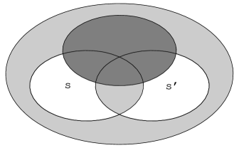
Figure 11: Clause selection for counting problems contributing to ${N_{\rm problems}}(\{r,s,s^{\prime}\},b,b^{\prime})$. The regions correspond to groups of the $M$ possible clauses based on their conflicts with $r$, $s$ and $s^{\prime}$. The dark gray region represents clauses that conflict with $r$ and so cannot be selected. The white regions represent clauses that conflict only with one of $s$ or $s^{\prime}$. Contributing problems consist of $m$ clauses such that $b$ and $b^{\prime}$ conflict only with $s$ and $s^{\prime}$, respectively, and the remaining $m-b-b^{\prime}$ clauses conflict with both $s$ and $s^{\prime}$ or with neither (light gray region).

The possible clause selection is illustrated in Fig. 11. For given assignments $r$, $s$ and $s^{\prime}$, group those clauses that do not conflict with $r$ as follows. Let ${N_{s}}$ and ${N_{s^{\prime}}}$ be the number of clauses that conflict only with $s$ and $s^{\prime}$, respectively, and ${N_{\rm other}}$ the number that do not conflict with $r$ and conflict with both or neither of $s$ and $s^{\prime}$ (the light gray region in Fig. 11). Then we have

$${N_{\rm problems}}(\{r,s,s^{\prime}\},b,b^{\prime})={{N_{s}}\choose b}{{N_{s^{\prime}}}\choose b^{\prime}}{{N_{\rm other}}\choose m-b-b^{\prime}}$$ (21)

as the number of problems for which $s$ and $s^{\prime}$ have, respectively, $b$ and $b^{\prime}$ unique conflicts, and $r$ is a solution.

Figure 12: Grouping of variables based on assigned values in $r$, $s$ and $s^{\prime}$, each shown as a horizontal box schematically indicating values assigned to each of the $n$ variables. In each assignment, the value given in $r$ to a variable is shown as white, while black indicates the opposite value. In this diagram, variables are grouped according to the differences in values they are given in the three assignments. For instance, the first group, consisting of $w$ variables, has those variables assigned the same value in all three assignments.

C.1.1 Clause Group Sizes

Now consider the $n$ variables in four mutually exclusive groups based on the values they are assigned in $r$, $s$ and $s^{\prime}$, as illustrated in Fig. 12:

1. the $w$ variables with the same values in all three assignments

2. the $x$ variables with the same value in $r$ and $s$, but opposite value in $s^{\prime}$

3. the $y$ variables with the same value in $s$ and $s^{\prime}$, opposite that of $r$

4. the $z$ variables with the same value in $r$ and $s^{\prime}$, but opposite value in $s$

As an example with $n=5$, suppose $r=00000$, $s=10011$ and $s^{\prime}=00111$. The first variable has the same assignment in $r$ and $s^{\prime}$, but the opposite value in $s$, and is the only such variable, so $z=1$. The second variable is the only one with the same value in all three assignments, so $w=1$. Similarly, $x=1$ and $y=2$.

Assignment $r$ conflicts with $n\choose k$ clauses leaving $M-{n\choose k}$ clauses available for selection. The principle of inclusion and exclusion [42] gives the number of available clauses that conflict with

• both $s$ and $s^{\prime}$ is the number that conflict with both $s$ and $s^{\prime}$ minus the number of those that also conflict with $r$:

  $${N_{\rm both}}={w+y\choose k}-{w\choose k}$$ (22a)

• $s$ only is

  $${N_{s}}={n\choose k}-{w+x\choose k}-{N_{\rm both}}$$ (22b)

• $s^{\prime}$ only is

  $${N_{s^{\prime}}}={n\choose k}-{w+z\choose k}-{N_{\rm both}}$$ (22c)

• both $s$ and $s^{\prime}$ or with neither is

  $${N_{\rm other}}={n\choose k}(2^{k}-1)-{N_{s}}-{N_{s^{\prime}}}$$ (22d)

Through the expressions of Eq. (C.1.1), ${N_{\rm problems}}(\{r,s,s^{\prime}\},b,b^{\prime})$ given in Eq. (21) depends on $w$, $x$, $y$ and $z$, but otherwise is independent of the choice of assignments $r$, $s$ and $s^{\prime}$. We denote this value as ${N_{\rm problems}}(x,y,z;b,b^{\prime})$ since $w=n-x-y-z$ is determined by the remaining group sizes. Furthermore, $d(r,s)=y+z$ and $d(r,s^{\prime})=x+y$. Thus, in Eq. (19) the sum over the assignments $s$ and $s^{\prime}$ becomes a sum over $x$, $y$ and $z$ times the number of ways to pick $s$ and $s^{\prime}$ with assigned values matching each other and those of $r$ as specified by the values of $w$, $x$, $y$ and $z$. This latter quantity is just the multinomial coefficient $n\choose w,x,y,z$. Finally, because the quantities in the sum depend on $w$, $x$, $y$ and $z$ but not the specific choice of the assignment $r$, the sums can be rearranged to move all terms outside of the sum over $r$. This leaves the inner sum as $\sum_{r}1$ which just counts the number of assignments, i.e., $2^{n}$, and cancels the factor $2^{-n}$ appearing in Eq. (19). Thus for the ensemble of random $k$-SAT, Eq. (19) becomes

$$\left\langle P_{\rm soln}\right\rangle=\sum_{xyz}{n\choose w,x,y,z}u_{y+z}u_{x+y}^{*}\sum_{bb^{\prime}}e^{i\pi\rho(b-b^{\prime})}\frac{{N_{\rm problems}}(x,y,z;b,b^{\prime})}{{N_{\rm problems}}}$$ (23)

C.1.2 An Example

To illustrate this counting argument, consider $n=3$, $k=2$ and $m=3$. This example has $M=12$ possible clauses and hence ${N_{\rm problems}}={12\choose 3}=220$. For assignments $r=000$, $s=011$ and $s^{\prime}=110$, how many of these problems have no conflicts with $r$, $b=1$ conflict only with $s$ and $b^{\prime}=2$ conflicts only with $s^{\prime}$? For these assignments, $w=0$, i.e., there are no variables with the same assigned value in all three assignments, and $x=y=z=1$. From Eq. (C.1.1), we then have ${N_{\rm both}}=0$ (no clauses conflict with both $s$ and $s^{\prime}$ since they share no pair of variables with the same values), ${N_{s}}={N_{s^{\prime}}}={3\choose 2}=3$ and ${N_{\rm other}}=3$.

Thus Eq. (21) gives ${N_{\rm problems}}(\{r,s,s^{\prime}\},1,2)=9$. An example is the problem with the following three clauses: $V_{1}$ OR (NOT $V_{2}$), (NOT $V_{1}$) OR (NOT $V_{2}$), and (NOT $V_{1}$) OR $V_{3}$. None of these clauses conflict with $r$. The first clause conflicts only with $s$, so $b=1$, and the last two conflict only with $s^{\prime}$, so $b^{\prime}=2$.

C.2 Asymptotic Behavior

For random $k$-SAT, Eq. (23) gives the exact value for $\left\langle P_{\rm soln}\right\rangle$. As $n\rightarrow\infty$, the discussion in §3.2 indicates the main contributions are from assignments with close to the average number of conflicts, ${c_{\rm avg}}=m/2^{k}$. That is, terms for which $b$ and $b^{\prime}$ are $\Theta\left(m\right)$. We thus use the scaled values $\hat{b}=b/m$ and $\hat{b^{\prime}}=b^{\prime}/m$ to simplify the analysis. Similarly the main contribution in the outer sum comes from values of $d(r,s)=y+z$ and $d(r,s^{\prime})=x+y$ close to $n/2$. This suggests defining $\hat{w}=w/n$,…,$\hat{z}=z/n$. As we will see below, these are indeed the appropriate scaling behaviors for the dominant contributions to the sum.

C.2.1 Sum over Conflicts

With $w,x,y,z$ scaling as $\Theta\left(n\right)$, the number of possible clauses $M$ and each value in Eq. (C.1.1) scale as ${n\choose k}=\Theta\left(n^{k}\right)$. This value is much larger than the actual number of clauses $m$ that appear in hard problems, for which $m=\Theta\left(n\right)$. We thus consider $1\ll m\ll n^{k}$. A convenient scaling for the numbers of available clauses is $\hat{N}_{\ldots}=N_{\ldots}/M$ so that

$${\hat{N}_{\rm both}} = \frac{(\hat{w}+\hat{y})^{k}-\hat{w}^{k}}{2^{k}}$$ (24)

$${\hat{N}_{s}} = \frac{1-(\hat{w}+\hat{x})^{k}}{2^{k}}-{\hat{N}_{\rm both}}$$

$${\hat{N}_{s^{\prime}}} = \frac{1-(\hat{w}+\hat{z})^{k}}{2^{k}}-{\hat{N}_{\rm both}}$$

$${\hat{N}_{\rm other}} = 1-2^{-k}-{\hat{N}_{s}}-{\hat{N}_{s^{\prime}}}$$

with corrections of order $1/n$.

When $S\ll\sqrt{R}$, ${R\choose S}\sim R^{S}/S!$. Using Stirling’s formula [1] with this expression then gives $e^{S+S\log(R/S)}/\sqrt{2\pi S}$. Thus for $m\ll n^{k/2}$, ${N_{\rm problems}}(x,y,z;b,b^{\prime})/{N_{\rm problems}}\sim e^{mX}m^{-1}Y$ where

$$X=\hat{b}\log\frac{{\hat{N}_{s}}}{\hat{b}}+\hat{b}^{\prime}\log\frac{{\hat{N}_{s^{\prime}}}}{\hat{b}^{\prime}}+(1-\hat{b}-\hat{b}^{\prime})\log\frac{{\hat{N}_{\rm other}}}{1-\hat{b}-\hat{b}^{\prime}}$$ (25)

and

$$Y=\frac{1}{2\pi\sqrt{\hat{b}\hat{b}^{\prime}(1-\hat{b}-\hat{b}^{\prime})}}$$ (26)

For the inner sum of Eq. (23), this quantity is multiplied by $\exp(i\pi m\rho(\hat{b}-\hat{b}^{\prime}))$ and summed over $b$ and $b^{\prime}$. When $m$ is large, this sum can be approximated by an integral over the scaled variables $\hat{b}$ and $\hat{b}^{\prime}$. Converting to an integral introduces a power of $m$ for each variable, so the inner sum is asymptotic to

$$m\int d\hat{b}\,d\hat{b}^{\prime}\,Y\exp(m(X+i\pi\rho(\hat{b}-\hat{b}^{\prime})))$$ (27)

The asymptotic behavior of this integral as $m\rightarrow\infty$ is readily evaluated by the method of steepest descents [2]. This involves considering complex values for the integration variables and noting that the value of the integral is dominated by its behavior around a stationary point, i.e., values for $\hat{b}$ and $\hat{b}^{\prime}$ for which $X+i\pi\rho(\hat{b}-\hat{b}^{\prime})$ has zero derivatives with respect to $\hat{b}$ and $\hat{b}^{\prime}$. Specifically, the integral is asymptotic to the value of the integrand at the stationary point multiplied by $2\pi m^{-1}/\sqrt{-\det D}$ where $D$ is the matrix of 2nd derivatives of $X+i\pi\rho(\hat{b}-\hat{b}^{\prime})$ evaluated at the stationary point, and $\det D$ is its determinant. Evaluating these derivatives then shows the inner sum is asymptotic to $\exp(mI)$ with

$$I=\log\left(e^{i\pi\rho}{\hat{N}_{s}}+e^{-i\pi\rho}{\hat{N}_{s^{\prime}}}+{\hat{N}_{\rm other}}\right)$$ (28)

which depends on $\hat{w},\ldots,\hat{z}$ through Eq. (24).

This derivation assumed $m\ll\sqrt{n^{k}}$. When $m$ is larger than this, the binomials give additional contributions. However, if $\rho$ is small, specifically of order $n/m$, these additions do not change the final asymptotic result. As described below, this behavior of $\rho$ is the appropriate choice for $m\gg n$ so we use this result over the full set of scaling behaviors for $m$.

C.2.2 Sum Over Variable Groupings

For the remaining sum in Eq. (23), over $x$, $y$ and $z$, Stirling’s formula gives

$${n\choose w,x,y,z}\sim\exp(nH)n^{-3/2}\sqrt{\frac{1}{(2\pi)^{3}\hat{w}\hat{x}\hat{y}\hat{z}}}$$ (29)

with the entropy

$$H=-\hat{w}\log\hat{w}-\ldots-\hat{z}\log\hat{z}$$ (30)

and $\hat{w}=1-\hat{x}-\hat{y}-\hat{z}$.

The $u_{y+z}u_{x+y}^{*}$ factors are $\exp(nU)$ with

$$U=2\beta_{C}+\beta(\hat{x}+2\hat{y}+\hat{z})+i\pi(\hat{x}-\hat{z})/2$$ (31)

where, from Eq. (8),

$$\beta_{C} = \log(\cos(\pi\tau/2))$$ (32)

$$\beta = \log(\tan(\pi\tau/2))$$

Combining these values with the result from the inner sum again gives a sum that can be approximated by an integral. After changing to scaled variables this becomes

$$\left\langle P_{\rm soln}\right\rangle\sim n^{3/2}\int d\hat{x}\,d\hat{y}\,d\hat{z}\,\sqrt{\frac{1}{(2\pi)^{3}\hat{w}\hat{x}\hat{y}\hat{z}}}\exp(n(H+U)+mI)$$ (33)

with $\hat{w}=1-\hat{x}-\hat{y}-\hat{z}$. The method of steepest descents applies to this integral. Thus, its asymptotic behavior is determined by the stationary point, namely the values of $\hat{x}$, $\hat{y}$ and $\hat{z}$ for which the derivatives of $n(H+U)+mI$ with respect to these three variables are zero. Let $\Delta$ be the corresponding $3\times 3$ matrix of 2nd derivatives and $A$ the value of $-(H+U+Im/n)$, both evaluated at this point. The asymptotic behavior is then

$$\left\langle P_{\rm soln}\right\rangle\sim\sqrt{\frac{-1}{\hat{w}\hat{x}\hat{y}\hat{z}\det\Delta}}\exp(-nA)$$ (34)

evaluated at the stationary point. These quantitites depend on the parameters $k$, $\mu=m/n$, $\rho$ and $\tau$.

The stationary point has no simple closed form but is readily evaluated numerically. For example, with $\mu=4$ and parameters $\tau=0.286$, $\rho=0.218$ used in Table 1, the stationary point is at $\hat{w}=0.710$, $\hat{x}=0.101+0.158i$, $\hat{y}=0.088$ and $\hat{z}=0.101-0.158i$ with $A=0.280$ and $\det\Delta=-478.5$, so $\left\langle P_{\rm soln}\right\rangle\sim 0.98e^{-0.28n}$, corresponding to the $\mu=4$ curve in Fig. 4.

C.3 Weakly Constrained Problems

When $1\ll m\ll n$, the decay rate $A=-(H+U+Im/n)$, can be treated through an expansion in the small quantity $\mu=m/n$. Specifically, the location of the stationary point for the variables $\hat{x}$, $\hat{y}$ and $\hat{z}$ is determined, to $\Theta\left(1\right)$, by setting the derivatives of $H+U$ to zero. The contribution from the sum over conflicts, $\mu I$, only introduces corrections of $O\left(\mu\right)$.

The expression $H+U$ evaluated at the $\Theta\left(1\right)$ values for the stationary point is zero, for any choice of the parameters $\rho$ and $\tau$. The $O\left(\mu\right)$ values and the contribution from $\mu I$ then give a scaling for $\left\langle P_{\rm soln}\right\rangle$ of $\exp(\Theta\left(m\right))$. However, for an appropriate choice of $\tau$ and $\rho$, the coefficient of this $\Theta\left(m\right)$ term can be set to zero, so that the actual scaling is dominated by the $\Theta\left(\mu^{2}\right)$ correction, i.e., $\exp(\Theta\left(n\mu^{2}\right))$ corresponding to the behavior seen in Fig. 5.

The parameter values eliminating the $\Theta\left(m\right)$ decay do not have a simple closed form. They are determined by trigonometric equations arising from setting to zero the derivatives of the $\Theta\left(m\right)$ contribution with respect to $\tau$ and $\rho$. The optimal choice for $\tau$ satisfies

$$2\cos^{k}\left(\frac{\pi\tau}{2}\right)\cos\left(k\frac{\pi\tau}{2}\right)=1$$ (35)

With this value for $\tau$, $\rho$ must then satisfy $\sin(\pi(\rho+k\tau))=0$. Among the many possible solutions for $\rho$ and $\tau$, we select the one in the range 0 to 1 for definiteness. For $k=3$ these equations give $\tau=0.201389$ and $\rho=0.395832$, which correspond to the limiting values in Fig. 2 as $m/n\rightarrow 0$.

These values of the parameters and the corresponding stationary point in Eq. (34) give $\left\langle P_{\rm soln}\right\rangle\sim e^{-{\alpha_{\rm weak}}m^{2}/n}$, where ${\alpha_{\rm weak}}$ is determined numerically, with the corresponding decay rate $A={\alpha_{\rm weak}}\mu^{2}$.

C.4 Highly Constrained Problems

For $m\gg n$, we focus on the ensemble of problems with a prespecified solution. In fact, with this many clauses, there are relatively few solutions in addition to the prespecified one. Thus a simpler evaluation considers the probability that the quantum search finds the prespecified solution, rather than any solution. This quantity is a lower bound on $\left\langle P_{\rm soln}\right\rangle$, and is a tight bound when $m\gg n$.

This lower bound is given by setting assignment $r$ in Eq. (19) to be the prespecified solution rather than summing over all possible assignments. The derivation leading to Eq. (23) proceeds as before except for two changes. First, eliminating the sum over $r$ gives an additional factor of $2^{-n}$. Second, the number of possible problems ${N_{\rm problems}}$ is replaced by

$$M-{n\choose k}\choose m$$ (36)

reflecting the smaller number of problems with a prespecified solution.

The asymptotic analysis gives an additional overall factor of $2^{-n}(1-2^{-k})^{-m}$. The resulting decay rate for $\left\langle P_{\rm soln}\right\rangle$ then has an upper bound given by the value of $-(H+U-\log 2+(I-\log(1-2^{-k}))m/n)$ evaluated at the corresponding stationary point.

For $m\gg n$, we can expand the stationary point evaluation in powers of $1/\mu$. Following the behavior for the optimal value of $\rho$ suggested by Fig. 2 and the values obtained in connection with Fig. 5, we take $\rho$ to be proportional to $1/\mu$. The $\Theta\left(1\right)$ values for the stationary point in this case are simply $\hat{x}=\hat{y}=\hat{z}=1/4$. Because $\rho\rightarrow 0$, the leading behavior for $I$ is just $\log(1-2^{-k})$ so the exponential scaling of $\Theta\left(m\right)$ is exactly zero. The contributions to the scaling of $\Theta\left(n\right)$ can be made equal to zero by selecting $\tau=1/2$ and $\rho=2^{k-2}(2^{k}-1)/(k\mu)$. The simple form for the $\Theta\left(1\right)$ stationary point values also allows evaluating the overall $\Theta\left(1\right)$ asymptotic behavior. Specifically, with these parameters, the scaling of the probability to find the prespecified solution is

$$\frac{4}{\sqrt{16+(k-1)^{2}\pi^{2}}}\exp\left(-\frac{(2^{k}-1)^{3}\pi^{2}}{16k^{2}}\frac{n^{2}}{m}\right)$$ (37)

The corresponding decay rate is $A=(2^{k}-1)^{3}\pi^{2}/(16k^{2}\mu)$.

References

- [1] M. Abramowitz and I. Stegun, editors. Handbook of Mathematical Functions. Dover, New York, 1965.
- [2] Carl M. Bender and Steven A. Orszag. Advanced Mathematical Methods for Scientists and Engineers. McGraw Hill, NY, 1978.
- [3] P. Benioff. Quantum mechanical hamiltonian models of Turing machines. J. Stat. Phys., 29:515–546, 1982.
- [4] Charles H. Bennett, Ethan Bernstein, Gilles Brassard, and Umesh V. Vazirani. Strengths and weaknesses of quantum computing. SIAM Journal on Computing, 26:1510–1523, 1997.
- [5] Ethan Bernstein and Umesh Vazirani. Quantum complexity theory. In Proc. 25th ACM Symp. on Theory of Computation, pages 11–20, 1993.
- [6] Andre Berthiaume, David Deutsch, and Richard Jozsa. The stabilization of quantum computations. In Proc. of the Workshop on Physics and Computation (PhysComp94), pages 60–62, Los Alamitos, CA, 1994. IEEE Press.
- [7] Eli Biham, Ofer Biham, David Biron, Markus Grassl, and Daniel A. Lidar. Grover’s quantum search algorithm for an arbitrary initial ampliltude distribution. Los Alamos preprint quant-ph/9807027 v2, June 1999.
- [8] Michel Boyer, Gilles Brassard, Peter Hoyer, and Alain Tapp. Tight bounds on quantum searching. In T. Toffoli et al., editors, Proc. of the Workshop on Physics and Computation (PhysComp96), pages 36–43, Cambridge, MA, 1996. New England Complex Systems Institute.
- [9] Gilles Brassard, Peter Hoyer, and Alain Tapp. Quantum counting. In K. Larsen, editor, Proc. of 25th Intl. Colloquium on Automata, Languages, and Programming (ICALP98), pages 820–831, Berlin, 1998. Springer. Los Alamos preprint quant-ph/9805082.
- [10] Nicolas J. Cerf, Lov K. Grover, and Colin P. Williams. Nested quantum search and NP-complete problems. In Applicable Algebra in Engineering, Communication and Computing. Springer, Berlin, 1998. Los Alamos preprint quant-ph/9806078.
- [11] Vladimir Cerny. Quantum computers and intractable (NP-complete) computing problems. Physical Review A, 48:116–119, 1993.
- [12] Peter Cheeseman, Bob Kanefsky, and William M. Taylor. Where the really hard problems are. In J. Mylopoulos and R. Reiter, editors, Proceedings of IJCAI91, pages 331–337, San Mateo, CA, 1991. Morgan Kaufmann.
- [13] Isaac L. Chuang, Neil Gershenfeld, and Mark Kubinec. Experimental implementation of fast quantum searching. Physical Review Letters, 80:3408–3411, 1998.
- [14] Isaac L. Chuang, Lieven M. K. Vandersypen, Xinlan Zhou, Debbie W. Leung, and Seth Lloyd. Experimental realization of a quantum algorithm. Nature, 393:143–146, 1998. Los Alamos preprint quant-ph/9801037.
- [15] James M. Crawford and Larry D. Auton. Experimental results on the crossover point in random 3SAT. Artificial Intelligence, 81:31–57, 1996.
- [16] Pedro S. de Souza and Saroush Talukdar. Asynchronous organizations for multi-algorithm problems. In Proc. of ACM Symposium on Applied Computing (SAC93), pages 286–294, Feb. 1993.
- [17] D. Deutsch. Quantum theory, the Church-Turing principle and the universal quantum computer. Proc. R. Soc. London A, 400:97–117, 1985.
- [18] D. Deutsch. Quantum computational networks. Proc. R. Soc. Lond., A425:73–90, 1989.
- [19] David P. DiVincenzo. Quantum computation. Science, 270:255–261, 1995.
- [20] R. P. Feynman. Quantum mechanical computers. Foundations of Physics, 16:507–531, 1986.
- [21] J. Frank, P. Cheeseman, and J. Stutz. When gravity fails: Local search topology. J. of Artificial Intelligence Research, 7:249–281, 1997.
- [22] M. R. Garey and D. S. Johnson. Computers and Intractability: A Guide to the Theory of NP-Completeness. W. H. Freeman, San Francisco, 1979.
- [23] Robert Gingrich, Colin P. Williams, and Nicolas Cerf. Generalized quantum search with parallelism. Los Alamos preprint quant-ph/9904049, JPL, 1999.
- [24] C. P. Gomes and B. Selman. Algorithm portfolio design: Theory vs. practice. In D. Geiger and P. Shenoy, editors, Proc. of the 13th Conf. on Uncertainty in AI (UAI-97), pages 190–197, Los Altos, CA, 1997. Morgan Kaufmann.
- [25] Ronald Graham, Oren Patashnik, and Donald E. Knuth. Concrete Mathematics: A Foundation for Computer Science. Addison-Wesley, Reading, MA, 2nd edition, 1994.
- [26] Lov K. Grover. Quantum computers can search arbitrarily large databases by a single query. Physical Review Letters, 79:4709–4712, 1997. Los Alamos preprint quant-ph/9706005.
- [27] Lov K. Grover. Quantum mechanics helps in searching for a needle in a haystack. Physical Review Letters, 78:325–328, 1997. Los Alamos preprint quant-ph/9706033.
- [28] Lov K. Grover. Quantum search on structured problems. Chaos, Solitons, and Fractals, 10:1695–1705, 1999.
- [29] Serge Haroche and Jean-Michel Raimond. Quantum computing: Dream or nightmare? Physics Today, 49:51–52, August 1996.
- [30] Tad Hogg. A framework for structured quantum search. Physica D, 120:102–116, 1998. Los Alamos preprint quant-ph/9701013.
- [31] Tad Hogg. Highly structured searches with quantum computers. Physical Review Letters, 80:2473–2476, 1998. Preprint at publish.aps.org/eprint/gateway/eplist/aps1997oct30_002.
- [32] Tad Hogg. Solving highly constrained search problems with quantum computers. J. of Artificial Intelligence Research, 10:39–66, 1999. Available at http://www.jair.org/abstracts/hogg99a.html.
- [33] Tad Hogg, Bernardo A. Huberman, and Colin Williams. Phase transitions and the search problem. Artificial Intelligence, 81:1–15, 1996.
- [34] Tad Hogg, Carlos Mochon, Eleanor Rieffel, and Wolfgang Polak. Tools for quantum algorithms. Intl. J. of Modern Physics C, 10:1347–1361, 1999. Los Alamos preprint quant-ph/9811073.
- [35] Peter Hoyer. Efficient quantum transforms. Los Alamos preprint quant-ph/9702028, February 1997.
- [36] Bernardo A. Huberman, Rajan M. Lukose, and Tad Hogg. An economics approach to hard computational problems. Science, 275:51–54, 1997.
- [37] Emanuel Knill, Raymond Laflamme, and Wojciech H. Zurek. Resilient quantum computation. Science, 279:342–345, 1998.
- [38] Rolf Landauer. Is quantum mechanically coherent computation useful? In D. H. Feng and B-L. Hu, editors, Proc. of the Drexel-4 Symposium on Quantum Nonintegrability, Boston, 1994. International Press.
- [39] Seth Lloyd. A potentially realizable quantum computer. Science, 261:1569–1571, 1993.
- [40] Christopher Monroe and David Wineland. Future of quantum computing proves to be debatable. Physics Today, 49:107–108, November 1996.
- [41] A. Nijenhuis and H. S. Wilf. Combinatorial Algorithms for Computers and Calculators. Academic Press, New York, 2nd edition, 1978.
- [42] E. M. Palmer. Graphical Evolution: An Introduction to the Theory of Random Graphs. Wiley Interscience, NY, 1985.
- [43] Eleanor G. Rieffel and Wolfgang Polak. An introduction to quantum computing for non-physicists. Los Alamos preprint quant-ph/9809016 TR-98-044, FXPAL, Sept. 8 1998. To appear in ACM Computing Surveys.
- [44] Bart Selman and Scott Kirkpatrick. Critical behavior in the computational cost of satisfiability testing. Artificial Intelligence, 81:273–295, 1996.
- [45] Bart Selman, Hector Levesque, and David Mitchell. A new method for solving hard satisfiability problems. In Proc. of the 10th Natl. Conf. on Artificial Intelligence (AAAI92), pages 440–446, Menlo Park, CA, 1992. AAAI Press.
- [46] P. Shor. Scheme for reducing decoherence in quantum computer memory. Physical Review A, 52:2493–2496, 1995.
- [47] Peter W. Shor. Algorithms for quantum computation: Discrete logarithms and factoring. In S. Goldwasser, editor, Proc. of the 35th Symposium on Foundations of Computer Science, pages 124–134, Los Alamitos, CA, November 1994. IEEE Press.
- [48] Neil Sloane. A Handbook of Integer Sequences. Academic Press, NY, 1973. On-line version available at http://www.research.att.com/njas/sequences.
- [49] Barbara M. Terhal and John A. Smolin. Single quantum querying of a database. Los Alamos preprint quant-ph/9705041 v4, IBM, Nov. 14 1997.
- [50] W. G. Unruh. Maintaining coherence in quantum computers. Physical Review A, 51:992–997, 1995.
- [51] Colin P. Williams and Tad Hogg. Exploiting the deep structure of constraint problems. Artificial Intelligence, 70:73–117, 1994.