Coherence properties of the stochastic oscillator

Abstract

An oscillator with stochastic frequency is discussed as a model for evaluating the quantum coherence properties of a physical system. It is found that the choice of jump statistics has to be considered with care if unphysical consequences are to be avoided. We investigate one such model, evaluate the damping it causes, the decoherence rate and the correlations it results in and the properties of the state for asymptotically long times. Also the choice of initial state is discussed and its effect on the time evolution of the correlations

I Introduction

The harmonic oscillator plays a pivotal role in the development of physics, both classical and quantum mechanical. It can be solved exactly, it displays a variety of non-trivial features and it has been applied successfully to a variety of phenomena.

A straightforward generalization of the simple oscillator is one with time dependent frequency; its Hamiltonian is

$$H=\frac{p^{2}}{2m}+\frac{1}{2}m\omega(t)^{2}x^{2}.$$ (1)

With a deterministic time evolution of $\omega(t),$ this can describe parametric frequency generation, radio-frequency traps or frequency modulated signal transmission. If, on the other hand, the frequency $\omega(t)$ is behaving in a random way, the model can be applied to a variety of physical situations, vide infra. The oscillator with a random frequency, has been the subject of a variety of theoretical approaches, see e.g. the review [1]. In quantum theory, the model (1) can be taken as an approximation to a situation where the oscillator is coupled to some degrees of freedom carrying out their quantum dynamics in a complicated fashion. Then it may be possible to model this by a time evolution so irregular that it can be regarded as stochastic.

With all quantum processes, we are not only interested in the time evolution of the averaged variables and their noise characterized by the dispersion from the averages. We also want to know how coherences are conserved, which variables retain their quantum character and how the classical behavior emerges. In this paper we undertake the task to investigate these questions for the oscillator, when $\omega(t)$ is given by a stochastic process.

Stochastic processes can be of two major types: In the one $\omega(t)$ varies continuously according to some model of the Brownian motion type or a modification of this. The ensuing theory is mathematically well understood, amenable to analytic approximations and often physically transparent. In another class of models, random telegraph signals called, the variable $\omega(t)$ jumps between constant values according to some stochastic rule. In simple cases, the consequences of such models can be evaluated [2], they have simple properties and they can be used as approximations for continuous behavior in the proper limit [3, 4]. In a quantum treatment, they offer the advantage that between the jumps, the well known properties of the harmonic oscillator can be applied directly. Thus we choose to utilize such a model here, and evaluate the influence the stochastic evolution has on the quantum coherence properties.

II Physical background

One application of a stochastic oscillator is to the s.c. continuous Stern-Gerlach measurement discussed by Dehmelt and his colleagues [5, 6, 7]. Here a trapped particle, an electron, sees two different trap potentials depending on the internal spin state. This is changing due to its own dynamics, and by monitoring the oscillational frequency of the charge, the experimentalist can see the frequency follow the changes of the internal spin state. This constitutes a continuous observation of the two quantum states, and the coherence between them cannot survive for any observable time, and a well defined frequency is always observed. This continuous Stern-Gerlach effect should be described by a stochastic quantum model along the lines developed by Carmichael and colleagues [8, 9]. They have been able to demonstrate how the monitoring of the state of a two level system gives precisely the type of well resolved jumping which is characteristic of the continuous Stern-Gerlach behavior. We have attempted such modelling, but the computational capacity needed was found to be unreasonably large, and hence we have settled on the stochastic process described above. This should suffice when one wants to investigate the consequences for the survival of quantum coherence in the oscillator.

Another situation where the time evolution is interrupted by change of the potential function governing the motion is given by molecular dynamics on adiabatic energy surfaces. Here spontaneous emission transfers a wave packet from an excited state to the ground state [10] or laser coupling may transfer the state back and forth between the potential levels. If this process is coherent, Rabi flopping may be observed [11] or adiabatic motion may ensue [12]. With less coherent coupling, the dynamic evolution has been described by surface hopping [13], where the deterministic motion on one potential surface is stochastically transferred to another one. It is well justified to describe this process by a random switch between the various potential curves. In this paper, the model assumes that the two harmonic states are situated directly above each other; this may not be a realistic description of a molecule, but it simplifies the treatment, and does not greatly affect the features we are investigating. It would not, in principle, be difficult to carry out the simulations on more realistic modifications of this model.

When an evolving quantum state is suddenly transferred to another potential at random times, we expect the quantum coherence to be obliterated, and the system to behave in a more classical way. This is seen in the density matrix in such a way that it tends towards the diagonal both in the position and the momentum representation. The uncertainties along the diagonal are then large, their product is expected to greatly exceed the minimum allowed by quantum theory. We have performed calculations to observe such disappearence of coherence.

The simplest model is to let the stochastic frequency jump between two values $\omega_{1}$ and $\omega_{2}$ with the constant jump probability $\nu.$ This model will be found to have physically less satisfactory features: The coherences decay, but the jumping process feeds energy into the system so efficiently that the energy grows at a rate quite comparable to the rate of vanishing of the coherences. The explanation for this strange behavior is in the physics of the oscillator motion. The system spends much of its time near the classical turning points of the oscillation, and consequently the jumps most likely take place here. Whenever the state jumps from the turning point of the flatter (slower) potential to the steeper (faster) one, it appears far up the potential slope, and a large increase in energy ensues. Jumping in the opposite direction, the system looses energy, but not enough to compensate for the gain. Thus the rapid increase in energy.

To overcome the unphysical features of our model, we strive to conserve energy in the jump process. This means that we have to favor jumping in the region where the change of potential energy is minimal, i.e. near the bottom of the wells. Thus the wave function should be most eager to jump, when it overlaps most with the ground state; then only the kinetic energy is transferred between the levels. This also maximizes the conservation of linear momentum; near the potential minimum, the motion most resembles free propagation.

In order to achieve the goal outlined above, we choose the following model: When the state on level $1$ is $\Psi_{1}(t)$, we jump to level $2$ with the probability

$$P_{12}(t)=\nu\mid\langle\Psi_{2}^{0}\mid\Psi_{1}(t)\rangle\mid^{2},$$ (2)

where $\Psi_{2}^{0}$ is the ground state of level $2.$ The jumps are taken to occur at a random time determined by $P_{12}$, and after that the state $\Psi_{1}(t)$ is transferred to level $2$ and evolved according to the corresponding potential. The probability to jump back to level $1$ is now determined by $P_{21}(t)$ given by the expression (2) with $1$ and $2$ interchanged. This simulation continues, and enough numerical data are accumulated to allow us to evaluate the ensemble averaged quantities. The results are then compared with those obtained by the simple model having $P=\nu$ constant.

III Time evolution of the state

The Schrödinger time evolution with the potential (1) is given by

$$i\hbar\frac{\partial}{\partial t}\Psi(x,t)=-\frac{\hbar^{2}}{2m}\frac{\partial^{2}\Psi(x,t)}{\partial x^{2}}+\frac{1}{2}m\omega_{i}^{2}x^{2}\Psi(x,t),$$ (3)

where $i=1$ or $2.$ Using the standard definition of the Wigner function [14]

$$W(X,P)=\frac{1}{2\pi\hbar}\int dx\;\langle X+\frac{x}{2}\mid\hat{\rho}\mid X-\frac{x}{2}\rangle\exp\left(-i\frac{Px}{\hbar}\right),$$ (4)

we can obtain the equation of motion

$$\frac{\partial W(X,P)}{\partial t}+\left(\frac{P}{m}\right)\frac{\partial W(X,P)}{\partial X}-m\omega_{i}^{2}X\;\frac{\partial W(X,P)}{\partial P}=0.$$ (5)

For the harmonic oscillator, this can be solved, and the various moments evaluated. It is, however, easy to see that the equations of motion for the moments close in each order, and their evolution equations can be obtained by simple calculations from that of the Wigner function. The mixed moments of the type $\langle xp\rangle$ denote symmetrized products, as these are given by the Wigner function.

The equations for the first moments we find to be the classical dynamic equations

$$\frac{d}{dt}\left(\begin{array}[]{r}\langle x(t)\rangle\\ \\ \langle p(t)\rangle\end{array}\right)=\left(\begin{array}[]{ccc}0&&\frac{1}{m}\\ &&\\ -m\omega^{2}&&0\end{array}\right)\left(\begin{array}[]{r}\langle x(t)\rangle\\ \\ \langle p(t)\rangle\end{array}\right).$$ (6)

For the second order ones we find

$$\frac{d}{dt}\left(\begin{array}[]{c}\langle x^{2}(t)\rangle\\ \langle p^{2}(t)\rangle\\ \langle x(t)p(t)\rangle\end{array}\right)=$$ (17)

$$\left(\begin{array}[]{ccccc}0&0&\frac{2}{m}\\ 0&0&-2m\omega^{2}\\ -m\omega^{2}&\frac{1}{m}&0\end{array}\right)\left(\begin{array}[]{c}\langle x^{2}(t)\rangle\\ \langle p^{2}(t)\rangle\\ \langle x(t)p(t)\rangle\end{array}\right)$$

Given the initial values, it is straightforward to integrate these equations for the moments. From these we can calculate the variances

$$\sigma_{x}^{2}(t) = \langle x^{2}(t)\rangle-\langle x(t)\rangle^{2}$$ (18)

$$\sigma_{p}^{2}(t) = \langle p^{2}(t)\rangle-\langle p(t)\rangle^{2}$$ (19)

$$\sigma_{xp}^{2}(t) = \langle x(t)p(t)\rangle-\langle x(t)\rangle\langle p(t)\rangle.$$ (20)

If the initial quantum state is a Gaussian wave function, it suffices to integrate the moments to the first two orders; it is known that the state will stay Gaussian, and that it is described by its moments of the first two orders. A straightforward calculation shows that the Schrödinger equation is satisfied by the state

$$\Psi(x,t)=(2\pi\sigma_{x}^{2}(t))^{-1/4}\exp(-\frac{(x-\langle x(t)\rangle)^{2}}{4\sigma_{x}^{2}(t)}+$$ (21)

$$\frac{i\sigma_{xp}^{2}(t)}{2\hbar\sigma_{x}^{2}(t)}(x-\langle x(t)\rangle)^{2}+\frac{i\langle p(t)\rangle}{\hbar}(x-\langle x(t)\rangle)+i\theta(t)),$$ (22)

where the phase $\theta(t)$ disappears in the calculation of the Wigner function (4) and thus does not affect the physics. All moments occurring in the state are not independent. If we start from a minimum uncertainty state, the combination

$$\sigma_{x}^{2}(t)\sigma_{p}^{2}(t)-\left(\sigma_{xp}^{2}(t)\right)^{2}=\frac{\hbar^{2}}{4}.$$ (23)

is conserved.

The density matrix in the position representation is given by $\langle x_{1}\mid\hat{\rho}\mid x_{2}\rangle,$ and its quantum coherence is the amount of off-diagonality, i.e. the dependence on the variable $x=x_{1}-x_{2}.$ Its moments can be evaluated directly from the Wigner function according to

$$\langle x^{n}\rangle = \int\int dx_{1}dx_{2}\left(x_{1}-x_{2}\right)^{n}\langle x_{1}\mid\hat{\rho}\mid x_{2}\rangle$$ (24)

$$= {2\pi(i\hbar)^{n}\int dR\left[\frac{\partial^{n}}{\partial P^{n}}W(R,P)\right]_{P=0}.}$$ (25)

A similar result can be obtained for the off-diagonality in the $p$-representation.

IV Numerical results

Starting from a Gaussian initial state, the equations (6) and (17) are integrated, and the state can be directly obtained from Eq.(22). We have found this integration to be orders of magnitude faster than the direct integration of Schrödinger’s equation, and obtaining the state from (22), we can directly calculate the Wigner function. The most time consuming part is still to accumulate enough single histories to obtain the ensemble averaged Wigner function and the corresponding average moments. This computation is, however, straightforward, and consists in simulating histories with the proper jump probabilities given as explained above. The whole calculation is time consuming but essentially trivial.

In the numerical work we want to evaluate the average position and momentum, and their variances. We have used dimensionless scaled units, which bring the numerical results into ranges of order unity. We have integrated the above problem using a Gaussian initial state on level $1$ with the initial values

$$\begin{array}[]{rrrrr}\langle x(0)\rangle=2.0&;&\langle p(0)\rangle=0&;&\\ \sigma_{x}^{2}(0)=0.5&;&\sigma_{p}^{2}(0)=0.5&;&\sigma_{xp}^{2}(0)=0.\end{array}$$ (26)

The stochastic model consists of jumping between the two frequencies $\omega_{1}=0.7$ and $\omega_{2}=1.2$ with the jump frequency parameter $\nu=0.8.$ We use two models, in the one the jump probabilities are constant

$$P_{12}=P_{21}=\nu,$$ (27)

in the other one we use the nonconstant, time dependent jump probabilities determined as explained in Sec.2 and Eq.(2). In order to get satisfactory statistics for evaluating the ensemble averages, the number of individual histories making up the ensemble consists of $N=30000$ runs.

In Fig. 1 we report the energy of the oscillator as function of dimensionless time. The solid line is the constant jump probability result, which displays a nearly exponential growth. The dotted line is the result with the nonconstant jump probability determined according to Eq.(2). We can see that the goal declared has been achieved; the energy grows much more slowly and clearly not exponentially. This is ascribed to the tendency of the nonconstant jump model to concentrate the jumping to the center of the potential.

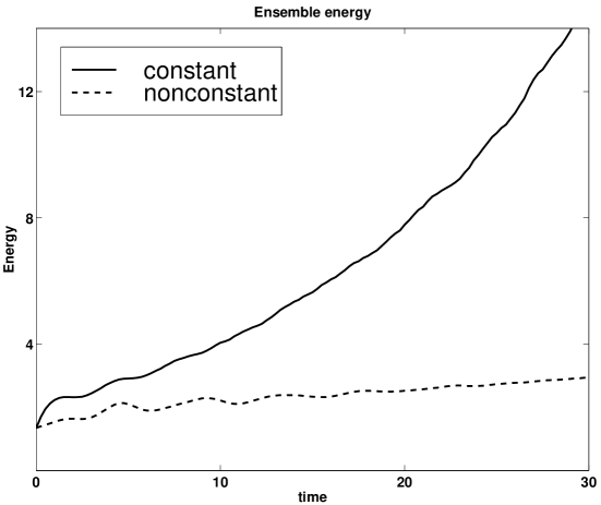
FIG. 1.: The ensemble energy as a function of time with constant and nonconstant jump probability. The jump frequency is $\nu=0.8$. The initial wavefunction is Gaussian with parameters $\langle X(0)\rangle=2.0$, $\langle P(0)\rangle=0.0$, $\langle\sigma_{X}^{2}(0)\rangle=0.5$, $\langle\sigma_{P}^{2}(0)\rangle=0.5$, $\langle\sigma_{XP}^{2}(0)\rangle=0.0$. The frequencies are $\omega_{1}=0.7$ and $\omega_{2}=1.2$. The initial frequency is $\omega_{1}$. The ensemble used is of size $N=30000$.

That this is, indeed, the case can be seen from Figs. 2 and 3. In Fig. 2 we show the statistical distribution of jumps from the level $1$ to $2.$ The classical turning points of the oscillational motion are indicated by the solid bars on the horizontal axis. The solid line shows the result for the constant probability, which leads to many jumps near or outside the turning points, where the oscillator spends large times. The peak at the right hand edge indicates the position of the starting wave packet. The dashed line is the result of the simulation with nonconstant probabilities. The jumps occur much closer to the center of the potentials as expected, even if the effect of the turning points is still seen. The total jump rate has decreased, thus the initial asymmetry is no longer so manifest.

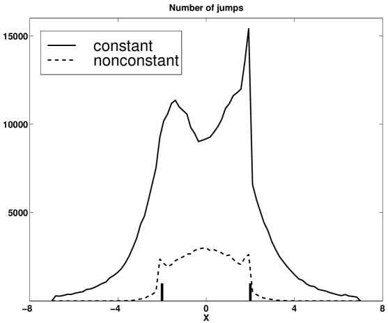
FIG. 2.: The number of jumps from the potential with $\omega_{1}$ to the potential with $\omega_{2}$. The bars on the $X$-axis show the classical turning points with the frequency $\omega_{1}$. The parameters are the same as in FIG. 1

In Fig. 3, the distribution of jumps from state $2$ to state 1 is shown. The constant probability case shown by the solid line still concentrate to outside the turning points in the steeper potential; these are again shown as solid bars. The symmetry is now in the opposite direction because, with the initial condition chosen, there must occur one initial jump to state $2$ before we can have a jump back. The dashed line shows the result for the model with nonconstant probabilities. The same features are seen as in the previous figure, but in this case of faster oscillations, the turning points have slightly enhanced effect.

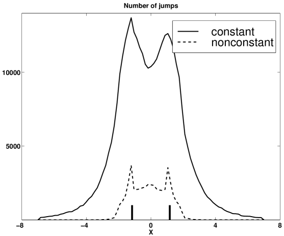
FIG. 3.: The number of jumps from the potential $\omega_{2}$ to $\omega_{1}$. The parameters are the same as in FIG. 1

The decrease of energy growth in the case of nonconstant jump probabilities allows the model to damp the average motion faster. This is seen in both the position variable, Fig. 4, and the momentum variable, Fig. 5. These variables are expected to behave in very similar manner for the harmonic motion. The damping time can be estimated to be of the order of $10$ units, which is much less than the one observed with constant probability.

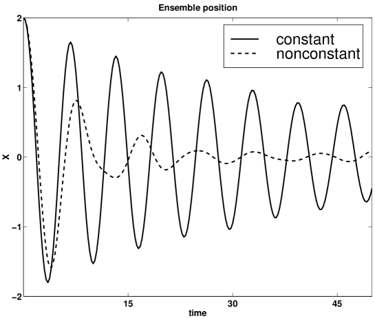
FIG. 4.: Ensemble position as a function of time. The parameters are the same as in FIG. 1

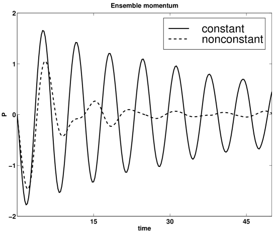
FIG. 5.: Ensemble momentum as a function of time. The parameters are the same as in FIG. 1

For harmonic motion, the second moments of both position and momentum are expected to grow like the energy, see Fig. 1. This is also seen in the variances; for constant probabilities they increase exponentially, while the nonconstant case grows more slowly. This is shown in Fig. 6, which should be compared with Fig. 1; the momentum variance behaves in a very similar manner.

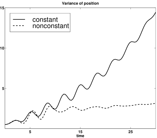
FIG. 6.: Position variance as a function of time. The parameters are the same as in FIG. 1

For the model with nonconstant jump probabilities, the time scale of motional damping has been found to be of order $10$, the range over which energy grows is several times this value, see Fig. 1. If we look at the dephasing causing the disappearance of quantum correlations in the position variable, we plot the expectation value

$$\langle x^{2}\rangle=\int\int dx_{1}dx_{2}\left(x_{1}-x_{2}\right)^{2}\langle x_{1}\mid\hat{\rho}\mid x_{2}\rangle,$$ (28)

which can be obtained directly from the Wigner function as shown in Eq. (25). The position density matrix can also be obtained from the Wigner function by inverting the relation (4)

$$\langle x_{1}\mid\hat{\rho}\mid x_{2}\rangle=\int dP\;\exp\left(\frac{iP(x_{1}-x_{2})}{\hbar}\right)\cdot$$ (29)

$$\hskip 28.45274ptW\left(\frac{(x_{1}+x_{2})}{2},P\right).$$ (30)

Fig. 7 shows the decay of the quantum mechanical correlations, and we can see that they disappear after a time of approximately $4$ units, which is considerably faster than the other time scales. In particular, the increase in energy is totally negligible over this time for the nonconstant jump probability; see Fig. 1. This clearly corrects the unphysical behavior of the model with constant probability. The constant model, on the other hand, destroys the quantum coherence about as fast as the other model does, but the asymptotic value for large times does not seem to vanish but linger on at a small but finite value. However, the very process of jumping removes the possibility to retain coherence, the actual statistics of the process seems to matter less.

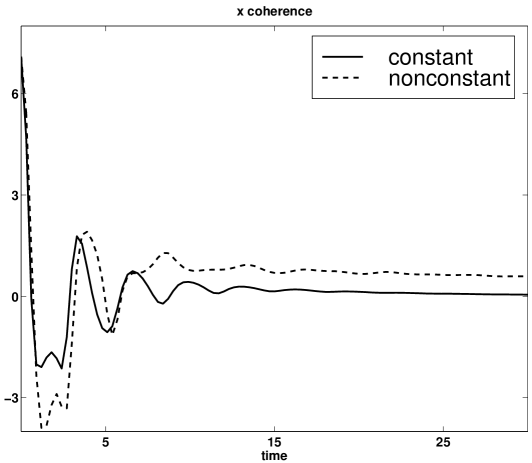
FIG. 7.: $X$-coherence as a function of time. The parameters are the same as in FIG. 1

When the harmonic oscillator is subjected to a random perturbation, we expect the final result to resemble a thermal distribution. In order to check this, we plot the density matrix in the occupation number representation. This is directly obtained from the position representation (30) using the relation

$$\langle n_{1}\mid\hat{\rho}\mid n_{2}\rangle=\int\int dx_{1}dx_{2}\langle n_{1}\mid x_{1}\rangle\langle x_{1}\mid\hat{\rho}\mid x_{2}\rangle\langle x_{2}\mid n_{2}\rangle.$$ (31)

The states $\langle x\mid n\rangle$ are the Hermit polynomial eigenstates of the harmonic oscillator, and the integrations in Eq.(31) are thus straightforward.

The diagonal elements of the density matrix in the occupation number representation with the frequency $\omega_{1}$ are shown in Fig. 8 for both models at the asymptotically large time $30$. We find that the model with nonconstant probability decreases much faster and goes to zero for large values of the quantum number. Both follow asymptotically an exponential decrease with the quantum number $n$.

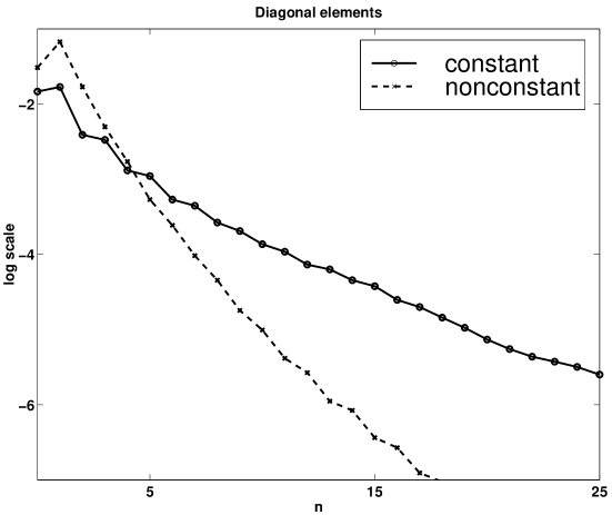
FIG. 8.: Diagonal elements of the ensemble energy density matrix $\langle m|\hat{\varrho}|n\rangle$ as a function of time. The Fock-states have the frequency $\omega_{1}$. The scale on the y-axis is logarithmic. The parameters are the same as in FIG. 1

The exponential decrease indicates that the state is close to a thermal distribution of the Planck type. However, the states near $n=0$ clearly deviate more than the following ones from a thermal distribution. This is verified when we follow the time evolution of the Wigner function in the $X,P-$plane. In Fig. 9, the original Gaussian state at $t=0$, rotates and distorts due to the influence of the jumping, which here is taken with nonconstant probabilities. The fore front rotates faster and the distribution loses phase information within a few units of the time. In Fig. 10, the time variable is $30$, and the phase information has disappeared. This picture corresponds to the same situation as that in Fig. 8, and the dip seen in the middle corresponds to the minimum at $n=0$ in that figure. It is obvious, that, in the occupation number representation, there are no off-diagonal density matrix elements in the state shown in Fig. 10.

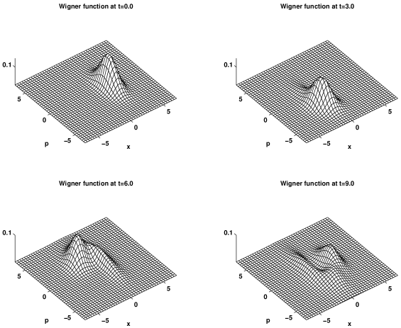
FIG. 9.: The Wigner function at four different times with a nonconstant jump probability. The parameters are the same as in FIG. 1

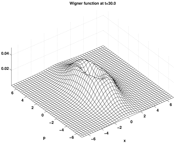
FIG. 10.: The Wigner function at $t=30.0$ with a nonconstant jump probability. The parameters are the same as in FIG. 1

V Effect of initial squeezing

The numerical results obtained so far have started from the ideal minimum uncertainty state (26). In order to see how sensitive our results are to this assumption, we have integrated the equations also with squeezed initial states. In the X-squeezed state we have set $\sigma_{X}^{2}(0)=0.25$ and $\sigma_{P}^{2}(0)=1.0$ ; in the P-squeezed state we have $\sigma_{X}^{2}(0)=1.0$ and $\sigma_{P}^{2}(0)=0.25.$ Fig. 11 reports the growth of energy in the model with nonconstant jump probabilities; compare this figure with Fig. 1. For the P-squeezed state, the advantages of letting the jump probability vary is partly lost; the X-squeezed case is not very different from that shown in Fig. 1. The wave packet still spends much time near the turning points, and in the case of P-squeezing at the initial point, the wave packet is very broad here. This increases the overlap with the central region of the oscillators, and the jumps adding energy to the system become more numerous.

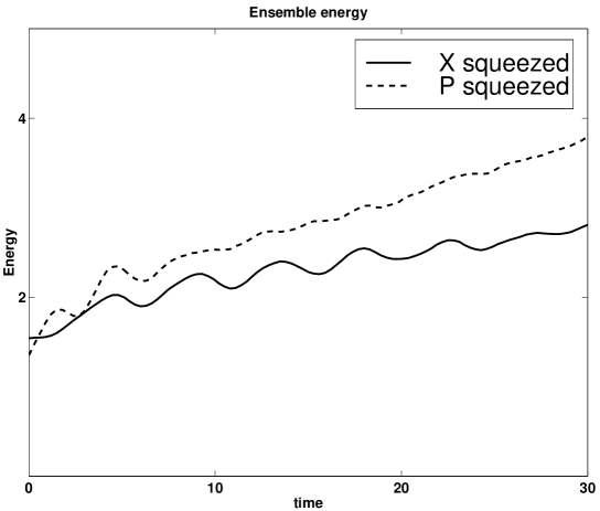
FIG. 11.: The ensemble energy as a function of time with X-squeezed $\sigma_{X}^{2}(0)=0.25$, $\sigma_{P}^{2}(0)=1.0$ and P-squeezed $\sigma_{X}^{2}(0)=1.0$, $\sigma_{P}^{2}(0)=0.25$ as initial conditions. The other parameters are the same as in FIG 1.

In Fig. 12 we show the jump distribution from the initial level $1$ to level 2, and we see that the P-squeezed state clearly tends to concentrate around the turning points. This figure should be compared with Fig. 2, and we can see that even the X-squeezed state has an enhanced jump probability as compared with the unsqeezed result, the dashed line in Fig. 2. Fig. 12, does not, however, show any asymmetry as found in the model with a constant probability. The jump frequency from level $2$ back to level $1$ shows a behavior almost identical to that of Fig. 12; the P-squeezed state tends to jump around the turning points, the distribution has a minimum at the center, which is not found in the case of X-squeezing.

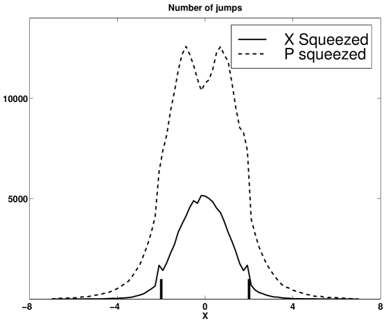
FIG. 12.: The number of jumps from the potential with $\omega_{1}$ to the potential with $\omega_{2}$. The bars on the x-axis show the classical turning points with the frequency $\omega_{1}$. The parameters are the same as in FIG. 12

Fig. 13 shows how the average position is decaying. There is little difference between the P- and X-squeezed cases, and only a slight decrease in the decay rate is seen when compared with the decay in Fig. 4. The average momentum behaves in a very similar way.

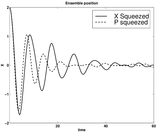
FIG. 13.: Ensemble position as a function of time. The parameters are the same as in FIG. 12

The variance in the position is shown in Fig. 14. For the case of X-squeezing, the wave packet is broad near the center, where the jumps take place, and the jumping consequently adds little width to the packet; the behavior is very similar to that of the dashed curve in Fig. 6 showing the result for the unsqueezed case. The P-squeezed case, however, jumps more often near the turning points, and consequently the width in position space is growing more rapidly. However, not by far as rapidly as with the constant jump probability shown in Fig. 6, the solid curve.

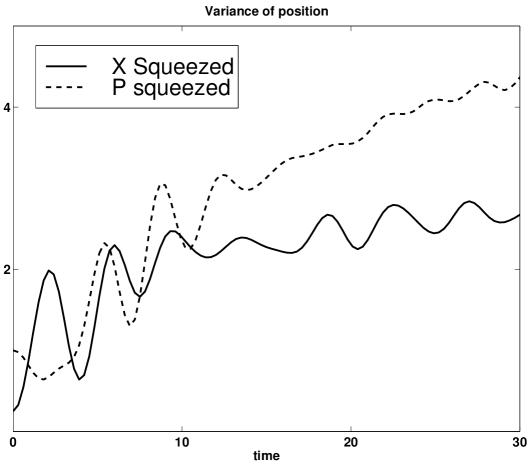
FIG. 14.: Position variance as a function of time. The parameters are the same as in FIG. 12

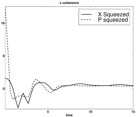
FIG. 15.: $X$-coherence as a function of time. The parameters are the same as in FIG. 12

When we look at the disappearance of the quantum coherence, the variable (28), the result in Fig. 15 shows that squeezing does not affect the rate of disappearance of quantum coherence much as compared with Fig. 7. Jumping always destroys the coherence rapidly and efficiently as expected.

VI Conclusion

In this paper we have discussed the time evolution of quantum coherence and correlations in a harmonic oscillator with a stochastic frequency. For simplicity we choose a jump process, where the frequency stays constant but switches randomly according to a stochastic rule. In Sec.II of the paper we discuss the possible physical situations which may be modelled by such behaviour.

We find that one should be careful in modelling random jumping, because the enforced transitions violate energy conservation, which leads to clearly unphysical growth of the oscillator energy. In order to amend this shortcoming, we device an ad hoc model, where jumping near the potential minimum is enhanced, which tends to conserve energy. In addition, the motion resembles free propagation most closely at this point, and hence the jump achieves momentum conservation as close as possible, when we jump here. This gives some additional physical motivation to our model, when we consider it as an attempt to emulate the behaviour of real physical processes.

The model suggested is found to achieve the asserted goal: the energy grows but little, and the decoherence time scale is much shorter than that over which the energy changes. We find that jumping in itself tends to destroy quantum coherence, but jumping near the center of the potentials achieves this without a build-up of unphysical energy. After an asymptotically rather long time, the diagonal elements of the density matrix resembles that of a thermal state, but the occurrence of very low quantum numbers is less likely than it would be thermally. This is verified by plotting the Wigner function, which displays a ring shaped form resembling that of an operating laser. No phase information survives for large times.

We have always started the integration near one of the turning points. Squeezing the state in the P-direction, we find that the accompanying broadening in the X-direction leads to more jumps near the turning points. This trends to counteract the improvements introduced by our nonconstant jump probability model. With squeezing in the X-direction less ill effects are found. In this case, they would, however, be seen if we started the wave packet closer to the center of the potial.

We conclude that the model of a stochastic oscillator can be used to investigate the quantum coherences, but care has to be excersised when the model is chosen. In our work, we have shown how to achieve physically reasonable results with a suitably modified jump rate. Which model is appropriate in a given physical system must be left open; different situations may require different choices of jump statistics.

REFERENCES

- [1] N.G.Van Kampen, Phys.Rep 24 171 (1976)
- [2] N.G.Van Kampen, Stochastic Processes in Physics and Chemistry (North Holland) 1981
- [3] J.H.Eberly, K.Wodkiewicz, B.Shore: Phys.Rev.A 30 2381 (1984), Phys.Rev.A 30 2390 (1984)
- [4] K.Wodkiewicz, J.H.Eberly: Phys.Rev.A 31 2314 (1985), Phys.Rev.A 32 992 (1985)
- [5] Nobel Lectures, Physics 1981-1990 World Scientific 23 (1993)
- [6] H.Dehmelt, Am.J.Phys 58 17 (1990)
- [7] L.S.Brown, G.Gabrielse Rev.Mod.Phys 58 233 (1986)
- [8] H.J.Carmichael, P.Kochan, L.Tian Proceeding of the International Symposium of Coherent States: Past, Present and Future, edited by J.R.Klauder, World Scientific, Singapore (1993)
- [9] P.Kochan, H.J.Carmichael, P.R.Morrow, M.G.Raizen Phys. Rev. Lett. 75 45 (1995)
- [10] Wai Keung Lai, Stig Stenholm Optics Comm. 104 313 (1994)
- [11] A.Paloviita, K.-A.Suominen Phys. Rev. A 55 3007 (1997)
- [12] B.M.Garraway, K.-A.Suominen Phys. Rev. Lett. 80 932 (1998)
- [13] J.C.Tully, R.K.Puston J.Chem.Phys 55 562 (1971)
- [14] M.Hillery, R.F.O’Connel, M.O.Scully, E.P.Wigner Phys. Rep. 106 121 (1984)