Endoscopic Tomography and Quantum-Non-Demolition

Abstract

We propose to measure the quantum state of a single mode of the radiation field in a cavity—the signal field—by coupling it via a quantum-non-demolition Hamiltonian to a meter field in a highly squeezed state. We show that quantum state tomography on the meter field using balanced homodyne detection provides full information about the signal state. We discuss the influence of measurement of the meter on the signal field.

]

I Introduction

How to measure the quantum state of a single mode of the radiation field in a cavity? Various possibilities [2, 3, 4, 5, 6, 7, 8] offer themselves. However, a straightforward application of the method of quantum state tomography suggested in Ref. [9] and implemented experimentally in Refs. [10, 11, 12] does not work, since by coupling the field out of the resonator we change the field state. In the present paper we propose to couple the field via a quantum-non-demolition (QND) interaction [13] to a meter field on which we then perform tomography using a balanced homodyne detector. In this way we combine the idea of probing, that is doing endoscopy on the field without taking it out of the cavity, and the tool of tomography and arrive at the method of endoscopic quantum state tomography.

The goal of the present paper is to obtain information about the full quantum state of a single mode of the radiation field. To bring out the physics most clearly we assume that this field, referred to in the remainder of this article by the signal mode, is in a pure quantum state and neglect damping. We emphasize, however, that the method presented here also applies to a signal field described by a density operator. In contrast to the method of quantum state tomography [9, 10, 11, 12] based on homodyne detection, the present technique does not couple the signal field out of the resonator. In order to measure the signal field we couple it in a linear way to a meter field. Moreover, we couple both to a pump field. This allows us to achieve a quantum-non-demolition Hamiltonian describing the interaction between the signal and the meter mode. The use of a QND-Hamiltonian suggests that one might be able to arrange the scheme in such a way as to measure a complete quadrature distribution without re-preparing the quantum state. In other words, repeated measurements on the meter change the signal state but keep the quadrature distribution invariant. We show that unfortunately this is not the case. This is closely related to the question if the wave function of a single quantum system could be measured [14]. Indeed Ref. [15] suggests that the wave function of a single quantum system could be measured by employing a series of “protective measurements” where an a priori knowledge of the wave function enables one to measure this wave function and protect it from changing at the same time. However, Alter and Yamamoto [16] showed that a series of repeated weak quantum non-demolition measurements gives no information about the wave function of the system. The same authors [17] have also argued that it is not allowed to measure the full state of a single quantum system. Recently, D’Ariano and Yuen [18] have independently proven the impossibility of measuring the wave function of a single quantum system. The present intentions are much less ambitious since, eventually, we do not want to measure the full state of a single quantum system, but only the quadrature probability distribution.

The article is organized as follows: In Sec. II we re-derive the relevant QND Hamiltonian emphasizing its dependence on the phase of the pump field which allows us to probe all quadratures of the signal field. We devote Sec. III to the calculation of the entangled state of meter and signal originating from the unitary time evolution due to the QND Hamiltonian. In Sec. IV we study the influence of the measurement of the meter on the signal field and in Sec. V we consider two special cases: in phase and out of phase measurements. In Sec. VI we then turn to the question of tomography using a QND Hamiltonian. In Sec. VII we give a general argument which shows the impossibility of having a (QND) measurement which simultaneously keeps the probability distribution unchanged and gives information about the measured observable. We conclude in Sec. VIII by summarizing our main results. In order to keep the article self-contained we have included all relevant calculations but have summarized longer ones in Appendices A and B.

II QND Hamiltonian

In the present section we derive the QND Hamiltonian used in our tomographic scheme to couple the signal to the meter field. This treatment brings out clearly how the phase of the pump field allows us to probe every quadrature of the signal.

Our model starts from the Hamiltonian

$$\hat{H}\equiv i\hbar\chi[\hat{a}_{s}^{\dagger}\hat{a}_{m}^{\dagger}\hat{a}_{p}-\hat{a}_{s}\hat{a}_{m}\hat{a}_{p}^{\dagger}]+i\hbar\sigma[\hat{a}_{s}^{\dagger}\hat{a}_{m}-\hat{a}_{s}\hat{a}_{m}^{\dagger}]\;,$$ (1)

where $\hat{a}_{s}(\hat{a}_{s}^{\dagger})$, $\hat{a}_{m}(\hat{a}_{m}^{\dagger})$, and $\hat{a}_{p}(\hat{a}_{p}^{\dagger})$ denote the annihilation (creation) operators of the signal, meter, and pump field, respectively. The parameters $\chi$ and $\sigma$ measure the coupling between the three fields, and the meter and signal field, respectively.

A possible scheme of the measurement strategy suggested in this paper is shown in Fig. 1. We assume that the crystal is present in the cavity when we prepare the signal field. In this case the pump and the meter field are in vacuum states and the resulting modifications on the signal due to the presence of the crystal can be easily taken into account.

When the pump field is highly excited we can describe it by a coherent state of amplitude $\alpha$ and phase $2\phi$, that is

$$\hat{a}_{p}\simeq\alpha e^{2i\phi}\;.$$ (2)

Here we have defined the phase $2\phi$ rather than $\phi$ as to simplify the resulting equations. It is the variation of this phase $\phi$ of the pump field which allows us to perform tomography on the signal field. To understand this in more detail we substitute the coherent state approximation, Eq. (2), of the pump field into the Hamiltonian, Eq. (1), and find after minor algebra

$$\hat{H}=2\hbar\sigma\hat{x}_{s}(\phi+\pi/2)\cdot\hat{x}_{m}(\phi)\;.$$ (3)

Here we have arranged the strength $\alpha$ of the pump field such that $\chi\alpha=\sigma$. Moreover, we have introduced the quadrature operators

$$\hat{x}_{j}(\theta)\equiv\frac{1}{\sqrt{2}}\left(\hat{a}_{j}e^{-i\theta}+\hat{a}_{j}^{\dagger}e^{i\theta}\right)$$ (4)

of the signal $(j=s)$ and the meter $(j=m)$ mode at the angle $\theta$.

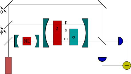
FIG. 1.: Possible scheme for endoscopic tomography. Our goal is to measure the density operator of the signal $s$ without taking the field out of the resonator. For this purpose, we couple it via a nonlinear medium of susceptibility $\chi$ to a pump and a meter field, $p$ and $m$, respectively. The meter field is in a squeezed state created for example in a separate resonator by another nonlinear medium NL. The pump field is in a coherent state of large amplitude $\alpha$ and phase $\phi$. The phase $\epsilon$ of the squeezing parameter is identical to $\phi$. Apart from the nonlinear coupling between signal and meter, there is also a linear coupling between the two. When the susceptibility $\sigma$ is equal to the product $\chi\alpha$, the effective interaction Hamiltonian for signal and meter is the product of two quadrature operators of the two fields. In particular, the two operators are out of phase and their average phase is set by the pump field. Using part of the pump field as a local oscillator with phase $\theta$, we perform a balanced homodyne detection on the meter coupled out of the resonator. When the homodyne phase $\theta$ is equal to the pump phase $\phi$ the interaction displaces the state of the signal field along the momentum axis and therefore leaves the position distribution invariant. Moreover, in this case the measured meter distribution is not influenced by the interaction with the signal. Since we have only displaced the quantum state of the signal, we have disturbed it in a controlled way. Unfortunately, we have not obtained any information about it. When the homodyne phase $\theta$ is out of phase with the pump phase $\phi$ the interaction changes the signal as well as the meter field . We therefore obtain information about the signal field but also disturb it. Consequently, we have to reprepare all quantum states after each measurement. To reconstruct the quantum state of the signal using tomography, we record the quadrature distributions of the meter for all phase angles $0<\theta<\pi$. In these measurements the homodyne phase $\theta$ has to be locked to the pump phase $\phi$ such that $\theta=\phi+\pi/2$.

Note that due to the special choice $\chi\alpha=\sigma$ of the pump field we have achieved an interaction between the signal and the meter which couples the quadrature operator $\hat{x}_{m}(\phi)$ of the meter at phase angle $\phi$ to the out-of-phase quadrature operator $\hat{x}_{s}(\phi+\pi/2)$ of the signal. Such Hamiltonians have been studied extensively [19, 20, 21, 22, 23, 24, 25] in the context of quantum non-demolition measurements. In the present paper we analyze how such a Hamiltonian can be used to measure the quantum state of the signal field. We note that according to the QND Hamiltonian Eq. (3) a measurement of the meter at a fixed phase $\phi$ of the pump field provides information about the signal in the out of phase quadrature. By varying the phase $\phi$ of the pump field we can probe in this way all quadratures of the signal. We conclude this section by noting that we can achieve a measurement of the meter quadrature operator by a homodyne measurement of the meter mode.

III Entanglement

We now calculate the combined state $|\Psi\rangle$ of signal and meter obtained from the QND interaction Hamiltonian, Eq. (3).

When we couple the signal and meter mode prepared initially in the states $|\psi_{s}\rangle$ and $|\psi_{m}\rangle$ we find the quantum state

$$|\Psi(t)\rangle = \exp(-i\hat{H}t/\hbar)|\psi_{m}\rangle|\psi_{s}\rangle$$ (5)

$$= \exp[-2i\sigma t\hat{x}_{s}(\phi+\pi/2)\hat{x}_{m}(\phi)]|\psi_{m}\rangle|\psi_{s}\rangle$$ (6)

for the combined system after the interaction time $t$. This time is determined by the decay time of the cavity.

To evaluate the above expression we expand the initial signal state in quadrature states $|x_{s}(\phi+\pi/2)\rangle$ of the phase angle $\theta_{s}\equiv\phi+\pi/2$, that is

$$|\psi_{s}\rangle=\int\limits_{-\infty}^{\infty}dx_{s}\,\psi_{s}(x_{s};\phi+\pi/2)|x_{s}(\phi+\pi/2)\rangle\;.$$ (7)

We emphasize that this representation and, in particular, the wave function $\psi_{s}(x_{s};\phi+\pi/2)\equiv\langle x_{s}(\phi+\pi/2)|\psi_{s}\rangle$ depend crucially on the angle $\theta_{s}$.

We substitute the expression Eq. (7) for the signal state into Eq. (6), use the eigenvalue equation

$$\hat{x}_{s}(\theta)|x_{s}(\theta)\rangle=x_{s}|x_{s}(\theta)\rangle$$ (8)

for the signal quadrature state $|x_{s}(\theta)\rangle$ at angle $\theta$, and arrive at the combined state

$$|\Psi(t)\rangle=\int\limits_{-\infty}^{\infty} dx_{s} \psi_{s}(x_{s};\phi+\pi/2)|x_{s}(\phi+\pi/2)\rangle$$ (9)

$$\times \exp[-2i\sigma tx_{s}\hat{x}_{m}(\phi)]|\psi_{m}\rangle$$ (10)

of signal and meter.

To find the action of the exponential operator in Eq. (10) on the meter state $|\psi_{m}\rangle$ it is convenient to expand $|\psi_{m}\rangle$ in quadrature states $|x_{m}(\theta)\rangle$ of the meter at the angle $\theta$, that is

$$|\psi_{m}\rangle=\int\limits_{-\infty}^{\infty}dx_{m}\,\psi_{m}(x_{m};\theta)|x_{m}(\theta)\rangle\;,$$ (11)

where $\psi_{m}(x_{m};\theta)\equiv\langle x_{m}(\theta)|\psi_{m}\rangle$ denotes the wave function of the meter state at the angle $\theta$. Note that this angle is still arbitrary and is not necessarily identical to the angle $\phi$ in the Hamiltonian. According to the Appendices A and B we find

$$\exp [-i(2\sigma tx_{s})\hat{x}_{m}(\phi)]|\psi_{m}\rangle$$ (12)

$$= \int\limits_{-\infty}^{\infty}dx_{m}\exp[-i\gamma(x_{s},x_{m};\theta-\phi)]$$ (13)

$$\times \psi_{m}[x_{m}-2\sigma tx_{s}\sin(\theta-\phi);\theta]|x_{m}(\theta)\rangle\;,$$ (14)

where

$$\gamma(x_{s},x_{m};\theta-\phi) \equiv (\sigma tx_{s})^{2}\sin[2(\theta-\phi)]$$ (16)

$$+2\sigma tx_{s}x_{m}\cos(\theta-\phi)$$

denotes the phase accumulated due to the interaction.

Hence the combined quantum state reads

$$|\Psi(t)\rangle = \int\limits_{-\infty}^{\infty}dx_{s}\int\limits_{-\infty}^{\infty}dx_{m}\psi_{s}(x_{s};\phi+\pi/2)$$ (20)

$$\quad\quad\times\psi_{m}[x_{m}-2\sigma tx_{s}\sin(\theta-\phi);\theta]$$

$$\quad\quad\times\exp[-i\gamma(x_{s},x_{m};\theta-\phi)]$$

$$\qquad\times|x_{s}(\phi+\pi/2)\rangle|x_{m}(\theta)\rangle\;.$$

We note that due to the coupling between the meter and the signal via the Hamiltonian Eq. (3), the meter wave function $\psi_{m}(x_{m};\theta)$ at the angle $\theta$ gets shifted by an amount $\delta x_{m}\equiv 2\sigma tx_{s}\sin(\theta-\phi)$. This shift is proportional to the interaction strength $\sigma t$, the signal variable $x_{s}$ and the sine of the angle $\theta-\phi$.

IV Signal state conditioned on meter measurement

In the preceding section we have calculated the entangled state $|\Psi\rangle$, Eq. (20), of the combined system. In the present section we show how a measurement of the meter influences the state of the signal. In particular, we use the Wigner function approach to discuss the properties of the signal state conditioned on a quadrature measurement of the meter variable. Here we first consider an arbitrary quadrature state of phase angle $\theta$ and then in Sec. V focus the discussion on two special cases.

According to Eq. (20) the conditioned state

$$|\psi_{s}^{(c)}\rangle=\frac{1}{\sqrt{W(x_{m})}}\langle x_{m}(\theta)|\Psi(t)\rangle$$ (21)

of the signal given that our quadrature measurement at angle $\theta$ has provided the value $x_{m}$ reads

$$|\psi_{s}^{(c)}\rangle=\int\limits_{-\infty}^{\infty}\,dx_{s}\psi_{s}(x_{s};\phi+\pi/2)f(x_{s}|x_{m})|x_{s}(\phi+\pi/2)\rangle\;,$$ (22)

where the filter function

$$f(x_{s}|x_{m}) = \frac{1}{\sqrt{W(x_{m})}}\psi_{m}[x_{m}-2\sigma tx_{s}\sin(\theta-\phi);\theta]$$ (23)

$$\times \exp[-i\gamma(x_{s},x_{m};\theta-\phi)]$$ (24)

originates from the interaction of the signal with the meter. The probability $W(x_{m})$ of finding the meter variable $x_{m}$ follows from the normalization condition

$$1=\langle\psi_{s}^{(c)}|\psi_{s}^{(c)}\rangle\;,$$ (25)

that is

$$W(x_{m})=\int\limits_{-\infty}^{\infty} dx_{s} |\psi_{s}(x_{s};\phi+\pi/2)|^{2}$$ (26)

$$\times |\psi_{m}[x_{m}-2\sigma tx_{s}\sin(\theta-\phi);\theta]|^{2}\;.$$ (27)

Equation (22) clearly shows how the measurement of the meter influences the quantum state of the signal: The filter function determined by the wave function of the meter selects those parts of the signal wave function that are entangled with the corresponding parts in the meter. To study this in more detail we now calculate the Wigner function [26]

$$W_{s}^{(c)}(x_{s},p_{s}|x_{m}) = \frac{1}{2\pi}\int\limits_{-\infty}^{\infty}dy\,e^{ip_{s}y}\langle x_{s}-y/2|\psi_{s}^{(c)}\rangle$$ (29)

$$\qquad\quad\times\langle\psi_{s}^{(c)}|x_{s}+y/2\rangle$$

of the signal state conditioned on the measured meter value $x_{m}$. For the sake of simplicity we have suppressed the angle $\phi+\pi/2$ at the quadrature states $|x+y/2\rangle$ and $|x-y/2\rangle$. Substituting the state $|\psi_{s}^{(c)}\rangle$, Eq. (22), into this expression we arrive at

$$W {}_{s}^{(c)}(x_{s},p_{s}|x_{m})=\frac{1}{2\pi}\int\limits_{-\infty}^{\infty}dy\,e^{ip_{s}y}\psi_{s}(x_{s}-y/2)$$ (30)

$$\times \psi_{s}^{\ast}(x_{s}+y/2)f(x_{s}-y/2|x_{m})f^{\ast}(x_{s}+y/2|x_{m})\;.$$ (31)

We express the integral as the convolution [27]

$$W_{s}^{(c)}(x_{s},p_{s}|x_{m})=$$ (32)

$$\qquad\int\limits_{-\infty}^{\infty}dp^{\prime}\,W_{s}(x_{s},p_{s}-p^{\prime})W_{f}(x_{s},p^{\prime}|x_{m})$$ (33)

between the Wigner function

$$W_{s}(x_{s},p_{s})=$$ (34)

$$\qquad\frac{1}{2\pi}\int\limits_{-\infty}^{\infty}dy\,e^{ip_{s}y}\psi_{s}(x_{s}-y/2)\psi_{s}^{\ast}(x_{s}+y/2)$$ (35)

of the original signal state and the Wigner function

$$W_{f}(x_{s},p_{s}|x_{m})=$$ (36)

$$\frac{1}{2\pi}\int\limits_{-\infty}^{\infty}dy\,e^{ip_{s}y}f(x_{s}-y/2|x_{m})f^{\ast}(x_{s}+y/2|x_{m})$$ (37)

of the filter provided by the meter measurement. We can easily prove Eq. (33) by substituting the expressions Eqs. (35) and (37) into Eq. (33), interchanging the integrations and performing one of them using the resulting delta function. We then indeed recover the integral (31).

If we substitute the filter function Eq. (24) into the Wigner function Eq. (37), after minor algebra we obtain

$$W_{f}(x_{s},p_{s}|x_{m})=\frac{1}{W(x_{m})}\frac{1}{2\pi}\int\limits_{-\infty}^{\infty}dy$$ (38)

$$\times\exp\{iy[p_{s}+2(\sigma t)^{2}x_{s}\sin[2(\theta-\phi)]+2\sigma tx_{m}\cos(\theta-\phi)]\}$$ (39)

$$\times\psi_{m}[x_{m}-2\sigma t\sin(\theta-\phi)(x_{s}-y/2)]$$ (40)

$$\times\psi_{m}^{\ast}[x_{m}-2\sigma t\sin(\theta-\phi)(x_{s}+y/2)]\;.$$ (41)

When we introduce in the last integral the new integration variable $\bar{y}\equiv 2\sigma t\sin(\theta-\phi)y$, and in the convolution Eq. (33) the integration variable $p\equiv p^{\prime}/[2\sigma t\sin(\theta-\phi)]$, the Wigner function of conditional state

$$W_{s}^{(c)}(x_{s},p_{s}|x_{m}) = \int\limits_{-\infty}^{\infty}dpW_{s}[x_{s},p_{s}-2\sigma t\sin(\theta-\phi)p]$$ (43)

$$\qquad\times W_{f}(x_{s},p|x_{m})$$

is the convolution of the Wigner function $W_{s}$ [Eq. (35)] of the signal state and the Wigner function

$$W_{f}(x_{s}, p |x_{m})=\frac{1}{W(x_{m})}\frac{1}{2\pi}\int\limits_{-\infty}^{\infty}d\bar{y}$$ (44)

$$\times \exp[i\bar{y}(p+2\sigma tx_{s}\cos(\theta-\phi)+x_{m}\cot(\theta-\phi))]$$ (45)

$$\times \psi_{m}(x_{m}-2\sigma tx_{s}\sin(\theta-\phi)+\bar{y}/2)$$ (46)

$$\times \psi_{m}^{\ast}(x_{m}-2\sigma tx_{s}\sin(\theta-\phi)-\bar{y}/2)$$ (47)

of the filter function. We express the latter in terms of the Wigner function

$$W_{m}(x_{m},p_{m})=$$ (48)

$$\frac{1}{2\pi}\int\limits_{-\infty}^{\infty}dy\,e^{ip_{m}y}\psi_{m}(x_{m}-y/2)\psi_{m}^{\ast}(x_{m}+y/2)$$ (49)

of the meter via the relation

$$W_{f}(x_{s} p|x_{m})=\frac{1}{W(x_{m})}W_{m}[x_{m}-2\sigma tx_{s}\sin(\theta-\phi);$$ , (50)

$$p +2\sigma tx_{s}\cos(\theta-\phi)+x_{m}\cot(\theta-\phi)]\;.$$ (51)

V Special examples for conditioned signal states

Whereas in the discussion of Sec. IV the angle $\theta$ of the meter quadrature is still arbritrary, we concentrate in the present section on two distinct cases: We choose (i) $\theta=\phi$, that is we measure in phase and (ii) $\theta=\phi+\pi/2$, that is out of phase measurement.

A In phase measurement

If we choose the angle $\theta$ of the meter quadrature to be identical to $\phi$, the state $|\Psi\rangle$, Eq. (20), of the complete system reduces to

$$|\Psi(t)\rangle = \int\limits_{-\infty}^{\infty}\,dx_{s}\int\limits_{-\infty}^{\infty}dx_{m}\psi_{s}(x_{s};\phi+\pi/2)\psi_{m}(x_{m};\phi)$$ (53)

$$\times\exp(-i2\sigma tx_{s}x_{m})|x_{s}(\phi+\pi/2)\rangle|x_{m}(\phi)\rangle\;.$$

Here we have made use of the phase $\gamma=2\sigma tx_{s}x_{m}$, Eq. (16), for $\theta=\phi$. Note that this expression also follows immediately from the Hamiltonian Eq. (3) and the expansions Eqs. (7) and (11) of the meter and signal states. We emphasize that in this case the meter wave function is not shifted. Nevertheless, the two states are still entangled via the exponential, Eq. (13). Since the shift $\delta x_{m}$ vanishes, the probability

$$W(x_{m})=|\psi_{m}|^{2}\int\limits_{-\infty}^{\infty}dx_{s}|\psi_{s}(x_{s})|^{2}=|\psi_{m}|^{2}\;,$$ (54)

of finding the meter variable $x_{m}$ following from Eq. (27) for $\theta=\phi$ is identical to the initial probability of the meter, that is

$$W(x_{m})=|\psi_{m}(x_{m})|^{2}\;.$$ (55)

Here we have used the fact that the original signal wave function is normalized. Hence, up to an overall phase $\mu_{m}$ determined by the meter wave function $\psi(x_{m})=|\psi(x_{m})|\exp[i\mu(x_{m})]$, we find from Eq. (24) the filter function $f(x_{s}|x_{m})=\exp(-i2\sigma tx_{s}x_{m})$, and from Eq. (22) the conditioned signal state

$$|\psi_{s}^{(c)}\rangle=\int\limits_{-\infty}^{\infty}\,dx_{s}\psi_{s}(x_{s})\exp(-i2\sigma tx_{s}x_{m})|x_{s}(\phi+\pi/2)\rangle\;.$$ (56)

Note that the measurement of the meter has indeed changed the state of the system but did not alter the probability

$$W(x_{s}) = |\langle x_{s}|\psi_{s}^{(c)}\rangle|^{2}=|\psi_{s}(x_{s})\exp(-i2\sigma tx_{s}x_{m})|^{2}$$ (57)

$$= |\psi_{s}(x_{s})|^{2}$$ (58)

of finding the signal variable $x_{s}$. This effect of the meter measurement comes out most clearly in the Wigner function $W_{s}^{(c)}$ of the conditioned system state, Eq. (33). From Eq. (41) we realize that for $\theta=\phi$ the Wigner function of the filter reduces to a delta function in the momentum shift, that is

$$W_{f}(x_{s},p_{s}|x_{m})=\delta(p_{s}+2\sigma tx_{m})\;,$$ (59)

and the Wigner function following from the convolution Eq. (33) reads

$$W_{s}^{(c)}(x_{s},p_{s}|x_{m})=W_{s}(x_{s},p_{s}+2\sigma tx_{m})\;.$$ (60)

Hence, the measurement has left untouched the shape of the original state represented here by the Wigner function but has moved it along the momentum axis by an amount of $2\sigma tx_{m}$. Consequently, the measurement did not change the probability distribution in the conjugate variable, namely the $x_{s}$ variable. We note, however, that in this way we cannot gain information about the signal since according to Eqs. (54) and (55) the probability distribution $W(x_{m})$ of measuring the variable $x_{m}$ is identical to the original distribution.

This finding is actually a rather general result. In fact, it can be rigorously shown [28] that a (QND) measurement which does not change the probability density of the observable which is being measured on a single quantum system gives no information about the measured observable. Its proof, restricted for clarity to the model considered here, can be found in Sec. VII.

B Out of phase measurement

We now turn to the case of $\theta=\phi+\pi/2$. In this case the shift $\delta x_{m}=2\sigma tx_{s}$ in the meter wave function is maximal and according to Eq. (16) the phase $\gamma$ vanishes. Hence, the combined state

$$|\Psi(t)\rangle=\int\limits_{-\infty}^{\infty}dx_{s}\int\limits_{-\infty}^{\infty}dx_{m}\psi_{s}(x_{s};\phi+\pi/2)$$ (61)

$$\times \!\psi_{m}(x_{m}-2\sigma tx_{s};\phi+\pi/2)\,|x_{s}(\phi+\pi/2)\rangle\,|x_{m}(\phi+\pi/2)\rangle$$ (62)

is an entangled state in which the entanglement between the meter and signal is due to the shift of the meter. In contrast to the discussion of Sec. V A we can now deduce properties of the signal from the shift of the meter wave function. Unfortunately, we cannot simultaneously keep the probability distribution $W(x_{s})=|\psi_{s}(x_{s})|^{2}$ of the original signal state invariant, in accordance with the discussion at the end of Sec. V A (see Sec. VII). Indeed, we find from Eqs. (22) or (56) the conditional state

$$|\tilde{\psi}_{s}^{(c)}\rangle=\frac{1}{\sqrt{\tilde{W}(x_{m})}}\;\int\limits_{-\infty}^{\infty}\!\!dx_{s}\,\psi_{s}(x_{s})\psi_{m}(x_{m}-2\sigma tx_{s})\,|x_{s}\rangle$$ (63)

of the system given the meter measurement at phase $\phi+\pi/2$ has provided the value $x_{m}$. The probability

$$\tilde{W}(x_{m})=\int\limits_{-\infty}^{\infty}dx_{s}|\psi_{s}(x_{s})|^{2}|\psi_{m}(x_{m}-2\sigma tx_{s})|^{2}$$ (64)

of finding the meter value $x_{m}$ following from Eq. (27) is now a convolution of the system and the meter function. In Sec. VI B we will use this relation to perform tomography on the system. However, in the present section we focus on how the measurement influences the signal state. We note that in contrast to the discussion of Sec. V A the meter measurement has changed the conditional distribution

$$\tilde{W}_{s}^{(c)} ( x_{s}|x_{m})=|\langle x_{s}|\psi_{s}^{(c)}\rangle|^{2}$$ (65)

$$= \!|\psi_{s}(x_{s})|^{2}\frac{|\psi_{m}(x_{m}-2\sigma tx_{s})|^{2}}{\int dx_{s}|\psi_{s}(x_{s})|^{2}|\psi_{m}(x_{m}-2\sigma tx_{s})|^{2}}\;.$$ (66)

of finding the signal variable $x_{s}$ given a measurement of the meter has provided $x_{m}$. Moreover, the Wigner function of the conditional system state is now given by

$$P^{(W)}(x_{s},p_{s}|x_{m}) = \frac{1}{\tilde{W}(x_{m})}\int\limits_{-\infty}^{\infty}dy\,e^{ip_{s}y}\psi_{s}^{\ast}\left(x_{s}+\frac{y}{2}\right)$$ (67)

$$\times \psi_{s}\left(x_{s}-\frac{y}{2}\right)\psi_{m}(x_{m}-2\sigma tx_{s}+\sigma ty)$$ (68)

$$\times \psi_{m}^{\ast}(x_{m}-2\sigma tx_{s}-\sigma ty)\;.$$ (69)

This Wigner function can again be expressed as the convolution

$$P^{(W)}(x_{s},p_{s}|x_{m})=\int\limits_{-\infty}^{\infty}dp^{\prime}\,W_{s}(x_{s},p_{s}-p^{\prime})W_{f}(x_{s},p^{\prime}|x_{m})\;,$$ (70)

where $W_{s}(x_{s},p_{s})$ is given by Eq. (35), and $W_{f}(x_{s},p_{s}|x_{m})$ this time reads

$$W_{f}(x_{s},p_{s}|x_{m}) = \frac{1}{2\pi\tilde{W}(x_{m})}\int\limits_{-\infty}^{\infty}dy\,e^{ip_{s}y}$$ (73)

$$\times\psi_{m}\left[x_{m}-2\sigma t\left(x_{s}-\frac{y}{2}\right)\right]$$

$$\times\psi_{m}^{\ast}\left[x_{m}-2\sigma t\left(x_{s}+\frac{y}{2}\right)\right]\;.$$

If we now change the variables $\bar{y}=2\sigma ty$ in Eq. (73) and $p=p^{\prime}/2\sigma t$ in Eq. (70), we can rewrite Eq. (70) as the convolution

$$P^{(W)}(x_{s},p_{s}|x_{m})=\int\limits_{-\infty}^{\infty}dpW_{s}(x_{s},p_{s}-2\sigma tp)W_{f}(x_{s},p|x_{m})$$ (74)

between the Wigner function of the signal state and the filter Wigner function

$$W_{f}(x_{s},p|x_{m}) = \frac{1}{2\pi\tilde{W}(x_{m})}\int\limits_{-\infty}^{\infty}dy\,e^{ipy}$$ (77)

$$\times\psi_{m}\left[x_{m}-2\sigma tx_{s}+\frac{y}{2}\right]$$

$$\times\psi_{m}^{\ast}\left[x_{m}-2\sigma tx_{s}-\frac{y}{2}\right]\;.$$

The latter can be expressed in terms of the Wigner function of the meter [Eq.(49)] via the relation

$$W_{f}(x_{s},p|x_{m})=\frac{1}{\tilde{W}(x_{m})}W_{m}(x_{m}-2\sigma tx_{s};p)\;.$$ (78)

Now, in contrast to Sec. V A, the filter Wigner function (78) does not reduce to a delta function, and therefore the Wigner function of the conditional signal state is not identical to the original one any more. This is indeed the effect of the measurement. This time, however, as we shall see in Sec. VI B, we can gain information about the signal.

VI Meter wave function

We continue considering the meter measurement at an angle $\theta=\phi+\pi/2$ but discuss two extreme cases: (i) The meter wave function is broad compared to the signal wave function and (ii) the meter wave function is extremely narrow. In the first case we do not change the signal state appreciably but can only learn about the lowest moments of the signal distribution. In contrast, the second way of making a measurement destroys the state but repeated measurements on an ensemble of systems all prepared in an identical way allow us to reconstruct the signal state using tomographic cuts.

A Weak measurements

Since $\psi_{m}$ is broad compared to $\psi_{s}$ we can evaluate $\psi_{m}$ at some characteristic value of $x_{s}$, such as $\langle x_{s}\rangle$. In this case the conditional state, Eq. (63), reduces to

$$|\psi_{s}^{(c)}\rangle\equiv\int\limits_{-\infty}^{\infty}dx_{s}\,\psi_{s}(x_{s})|x_{s}\rangle\;,$$ (79)

and the probability

$$\tilde{W}(x_{m})\equiv|\psi_{m}(x_{m}+2\sigma t\langle x_{s}\rangle)|^{2}$$ (80)

is the original meter probability shifted by an amount $2\sigma t\langle x_{s}\rangle$. Hence, when this shift $2\sigma t\langle x_{s}\rangle$ is larger than the width of $W_{m}(x_{m})=|\psi_{m}(x_{m})|^{2}$, we can learn about $\langle x_{s}\rangle$. As seen from Eq. (79), in this case the state of the signal mode does not change appreciably.

B Tomographic measurements

Optical homodyne tomography [9, 10, 11, 12, 29] is a method for obtaining the Wigner function (or, more generally [30, 31, 32], the matrix elements of the density operator in some representation) of the electromagnetic field, preparing the field again in the same state after each measurement. It therefore consists of an ensemble of repeated measurements of one quadrature operator for different phases relative to the local oscillator of the homodyne detector. However, the method first employed in Ref. [10] needs a smoothing procedure, because, in order to reconstruct the Wigner function one has to perform an integral involving the marginal probability distribution of homodyne measurement [9]. This was indeed performed in Refs. [10, 11] by methods which are standard in tomographic imaging [33].

In the present section we show that it is possible to perform tomography on the meter mode to obtain information about the signal state. To this end, we recall Eq. (64)

$$\tilde{W}(x_{m})=\int\limits_{-\infty}^{\infty}dx_{s}|\psi_{s}(x_{s})|^{2}|\psi_{m}(x_{m}-2\sigma tx_{s})|^{2}\;,$$ (81)

which gives the marginal distribution of the meter (probability distribution of the results of the measurements of $\hat{x}_{m}$) in the case of out of phase measurements. Let us assume that the meter wave function is extremely narrow, that is the meter is initially in a highly squeezed state, for example a squeezed vacuum $|0,\xi\rangle$, where $\xi=re^{i\epsilon}$ is the squeezing parameter. Then, according to Eq. (81), the marginal distribution $\tilde{W}(x_{m})$ is given by a convolution of the modulus square of the signal wave function with a narrow Gaussian

$$|\psi_{m}(x_{m} - 2\sigma tx_{s})|^{2}=\frac{1}{\sqrt{\pi}\cosh r(1-e^{i\epsilon}\tanh r)}$$ (82)

$$\times \exp\left\{-\left[\frac{1+e^{i\epsilon}\tanh r}{1-e^{i\epsilon}\tanh r}\right](x_{m}-2\sigma tx_{s})^{2}\right\}\;.$$ (83)

Now, if the modulus $r$ of the squeezing parameter is large enough, the Gaussian (82) approaches a delta function in the meter and signal variables

$$|\psi_{m}(x_{m}-2\sigma tx_{s})|^{2}\longrightarrow\frac{1}{|2\sigma t|}\delta\left(x_{s}-\frac{x_{m}}{2\sigma t}\right)\;,$$ (84)

and Eq. (81) reduces to

$$\tilde{W}(x_{m}) \cong \frac{1}{|2\sigma t|}\int\limits_{-\infty}^{\infty}dx_{s}\,|\psi_{s}(x_{s})|^{2}\delta\left(x_{s}-\frac{x_{m}}{2\sigma t}\right)$$ (86)

$$= \frac{1}{2\sigma t}\left|\psi_{s}\left(\frac{x_{m}}{2\sigma t}\right)\right|^{2}=\frac{1}{2\sigma t}W\left(\frac{x_{m}}{2\sigma t}\right)\;.$$ (87)

Hence, by measuring the probability distribution $\tilde{W}(x_{m})$ of the outcomes of the meter variable $x_{m}$ (for example via balanced homodyne detection performed on the meter field) we indirectly obtain the probability distribution $W(x_{s})$, up to a rescaling given by the factor $2\sigma t$. However, from Eq. (63) it is clear that in this case the signal wave function is changed, and therefore we need to prepare the signal field again in the same state after each measurement. This is what is usually done in quantum optical tomography [10, 11, 12].

The advantage of the present scheme is that we perform an indirect measurement: We do not detect the signal mode outside the cavity (that is, we do not have to take the signal field outside the cavity), but we couple it to a meter field which is successively detected, thus overcoming the smearing effect introduced by the direct detection of the signal [34]. Moreover, there is no need of a smoothing procedure, since we are interested in the marginal probability distribution $W(x_{s})$ which is directly related to $\tilde{W}(x_{m})$ through Eq. (84). In order to probe the full state of the signal field, however, we would need to measure the probability distribution $\tilde{W}(x_{m})$ for various values of the phase [9, 10, 11, 12, 30, 31, 32].

VII No measurement without a measurement

In this section we show that if a QND measurement performed on the signal does not alter the probability density of the measured observable, then the measurement process does not provide any information about the measured observable itself. In order to keep the paper self-contained, we prove this conclusion for the model considered here, but this argument holds true also in general, independently of the chosen model [28]. The argument is the following:

Let $\hat{\rho}_{s}(0)=|\psi_{s}(0)\rangle\langle\psi_{s}(0)|$ be the initial density matrix of the signal, and $\hat{x}_{s}$ the measured observable, with $\hat{x}_{s}|x_{s}\rangle=x_{s}|x_{s}\rangle$. The initial probability density one would like to preserve is $W_{s}^{0}(x_{s})=\langle x_{s}|\hat{\rho}_{s}(0)|x_{s}\rangle$, and we are interested in a QND measurement of $\hat{x}_{s}$. To this end, the signal is correlated to a meter which is initially in a certain state $|\psi_{m}\rangle$, and eventually a measurement is performed on the meter to yield the inferred measurement result $\bar{x}_{m}$. The measurement is then completely described [13] by the probability-amplitude operator

$$\hat{Y}(\hat{x}_{s},\bar{x}_{m})=\langle\bar{x}_{m}|\hat{U}(\hat{x}_{s},\hat{x}_{m})|\psi_{m}\rangle\;,$$ (88)

which accounts for the three stages of this measurement: preparation of the meter in the state $|\psi_{m}\rangle$, interaction between the meter and the signal to be measured through the unitary operator $\hat{U}(\hat{x}_{s},\hat{x}_{m})$ [see Eqs. (3) and (6)], and projection of the resulting entangled state onto the meter state $|\bar{x}_{m}\rangle$. The QND condition [13] for a back-action evading measurement then reads

$$[\hat{Y}(\hat{x}_{s},\bar{x}_{m}),\hat{x}_{s}]=0\;,$$ (89)

which means that $\hat{x}_{s}$ and $\hat{Y}$ share the same eigenstates:

$$\hat{Y}(\hat{x}_{s},\bar{x}_{m})|x_{s}\rangle = Y(x_{s},\bar{x}_{m})|x_{s}\rangle\;,$$ (91)

$$\hat{Y}^{\dagger}(\hat{x}_{s},\bar{x}_{m})|x_{s}\rangle = Y^{\ast}(x_{s},\bar{x}_{m})|x_{s}\rangle\;.$$ (92)

After a measurement which gives the result $\bar{x}_{m}$, the system is therefore described by the density matrix

$$\hat{\rho}_{s}=\frac{1}{W(\bar{x}_{m})}\hat{Y}(\hat{x}_{s},\bar{x}_{m})\hat{\rho}_{s}(0)\hat{Y}^{\dagger}(\hat{x}_{s},\bar{x}_{m})\;,$$ (93)

where

$$W(\bar{x}_{m}) = {\rm Tr}_{s}[\hat{Y}(\hat{x}_{s},\bar{x}_{m})\hat{\rho}_{s}(0)\hat{Y}^{\dagger}(\hat{x}_{s},\bar{x}_{m})]$$ (94)

$$= \int dx_{s}\,\langle x_{s}|\hat{Y}(\hat{x}_{s},\bar{x}_{m})\hat{\rho}_{s}(0)\hat{Y}^{\dagger}(\hat{x}_{s},\bar{x}_{m})|x_{s}\rangle$$ (95)

is the probability to obtain the result $\bar{x}_{m}$. Now, the probability density of the measured observable after the measurement is given by

$$W_{s}( x_{s} )=\langle x_{s}|\hat{\rho}_{s}|x_{s}\rangle$$ (96)

$$= \frac{1}{W(\bar{x}_{m})}\langle x_{s}|\hat{Y}(\hat{x}_{s},\bar{x}_{m})\hat{\rho}_{s}(0)\hat{Y}^{\dagger}(\hat{x}_{s},\bar{x}_{m})|x_{s}\rangle\;.$$ (97)

Applying the QND condition (89) and (89) we obtain

$$W_{s}(x_{s})=\frac{1}{W(\bar{x}_{m})}|Y(x_{s},\bar{x}_{m})|^{2}W_{s}^{(0)}(x_{s})\;.$$ (98)

If we require that this probability density does not change due to the measurement process, $W_{s}(x_{s})=W_{s}^{(0)}(x)$, then it must be that

$$|Y(x_{s},\bar{x}_{m})|^{2}=W(\bar{x}_{m})\;.$$ (99)

However, $W(\bar{x}_{m})$ is not a function of $x_{s}$ (the eigenvalues of the measured observable) and therefore also the eigenvalues $Y(x_{s},\bar{x}_{m})$ of $\hat{Y}(\hat{x}_{s},\bar{x}_{m})$ are independent of $x_{s}$. Since the operator $\hat{Y}$ describes the measurement process, if its eigenvalues are independent of the eigenvalues of $\hat{x}_{s}$, the measurement obviously gives no information about $\hat{x}_{s}$, unless the measured state is an eigenstate of the measured observable.

VIII Conclusions

In this paper we have proposed a method to measure the quadrature probability distribution (or, more generally, the full quantum state) of a single mode of the electromagnetic field inside a cavity. It is based on indirect homodyne measurements performed on a meter field which is coupled to the signal field via a QND interaction Hamiltonian. We have named this procedure “endoscopic tomography” because (i) it does not require (in contrast to Refs. [10, 11, 12]) to take the field out of the cavity, just as in “quantum state endoscopy” [2], where a beam of two-level atoms is used as a probe; (ii) tomographic measurements performed (by balanced homodyne detection) on the meter mode allow us to reconstruct the marginal probability distribution of the signal variable or even the full quantum state.

We have computed the entangled (signal-meter) state which arises during the evolution under the QND Hamiltonian, and evaluated the conditional signal state (given that a measurement on the meter has provided a certain result). Then, we have concentrated ourselves on two special cases, namely, in phase and out of phase measurements. We have shown that in the first case the shape of the Wigner function of the signal is not changed by the measurement, but also that such a measurement does not provide any information on the signal state. In the second case, however, we can get information about the signal, but its initial state is changed due to the measurement performed on the meter: in this case, preparing the signal field again in the same state after each measurement, balanced homodyne detection of the meter mode allows the reconstruction of the original signal state. Finally, we have given an argument according to which the results we have found in our model are rather general: a QND measurement which leaves unchanged the probability distribution of the system observable does not provide any information on the signal state.

A Displacement of the meter state

In this appendix we calculate the state

$$|\bar{\psi}_{m}\rangle\equiv\exp[-i2\sigma tx_{s}\hat{x}_{m}(\phi)]|\psi_{m}\rangle\equiv\hat{D}(\beta)|\psi_{m}\rangle$$ (A1)

which results from the application of the operator $\hat{D}(\beta)\equiv\exp[-i\beta\hat{x}_{m}(\phi)]$ on the meter state $|\psi_{m}\rangle$ with $\beta=2\sigma tx_{s}$. When we use the representation

$$|\psi_{m}\rangle=\int\limits_{-\infty}^{\infty}dx_{m}\psi_{m}(x_{m};\theta)|x_{m}(\theta)\rangle$$ (A2)

in quadrature states $|x_{m}(\theta)\rangle$ at the angle $\theta$, the state $|\bar{\psi}_{m}\rangle$ reads

$$|\bar{\psi}_{m}\rangle=\int\limits_{-\infty}^{\infty}dx_{m}\psi_{m}(x_{m};\theta)\exp[-i\beta\hat{x}_{m}(\phi)]|x_{m}(\theta)\rangle\;.$$ (A3)

We recall the result

$$\exp [-i\beta\hat{x}(\phi)]|x_{m}(\theta)\rangle=$$ (A4)

$$\exp \left\{-i\left[\frac{3\beta^{2}}{4}\sin\left[2(\theta-\phi)\right]+\beta x_{m}\cos(\theta-\phi)\right]\right\}$$ (A5)

$$\times |[x_{m}+\beta\sin(\theta-\phi)](\theta)\rangle$$ (A6)

derived in Appendix B and find

$$|\bar{\psi}_{m}\rangle = \int\limits_{-\infty}^{\infty}dx_{m}\psi_{m}(x_{m};\theta)$$ (A7)

$$\times \exp \left\{-i\left[\frac{3\beta^{2}}{4}\sin\left[2(\theta-\phi)\right]+\beta x_{m}\cos(\theta-\phi)\right]\right\}$$ (A8)

$$\times |[x_{m}+\beta\sin(\theta-\phi)](\theta)\rangle\;,$$ (A9)

which after introducing the integration variable $\bar{x}_{m}\equiv x_{m}+\beta\sin(\theta-\phi)$ reads

$$|\bar{\psi}_{m}\rangle = \int\limits_{-\infty}^{\infty}d\bar{x}_{m}\psi_{m}\left[\bar{x}_{m}-\beta\sin(\theta-\phi);\theta\right]$$ (A10)

$$\times \exp \left\{-i\left[\frac{\beta^{2}}{4}\sin\left[2(\theta-\phi)\right]+\beta\bar{x}_{m}\cos(\theta-\phi)\right]\right\}$$ (A11)

$$\times |\bar{x}_{m}(\theta)\rangle\;.$$ (A12)

Hence the meter wave function gets displaced and experiences a phase shift.

B Displacement of a quadrature state

In this appendix we derive the relation

$$e^{-i\beta\hat{x}(\theta)}|x(\theta^{\prime})\rangle = \exp\left[i\varphi(x;\beta,\theta^{\prime}-\theta)\right]$$ (B1)

$$\times |\left[x+\beta\sin(\theta^{\prime}-\theta)\right](\theta^{\prime})\rangle$$ (B2)

for the c-number $\beta$ and the quadrature operator

$$\hat{x}(\theta)\equiv\frac{1}{\sqrt{2}}(\hat{a}e^{-i\theta}+\hat{a}^{\dagger}e^{i\theta})\;.$$ (B3)

Here $\hat{a}$ and $\hat{a}^{\dagger}$ denote the annihilation and creation operators, respectively, with

$$[\hat{a},\hat{a}^{\dagger}]=1\;.$$ (B4)

Note that according to Eq. (B2) the action of the exponential of the quadrature operator $\hat{x}(\theta)$ at the angle $\theta$ on a quadrature eigenstate $|x(\theta^{\prime})\rangle$ at angle $\theta^{\prime}$ yields, apart from the phase

$$\varphi(x;\beta,\theta^{\prime}-\theta)=-\frac{3\beta^{2}}{4}\sin[2(\theta^{\prime}-\theta)]-\beta x\cos(\theta^{\prime}-\theta)\;,$$ (B5)

again a quadrature eigenstate at the angle $\theta^{\prime}$, but with the eigenvalue

$$x^{\prime}\equiv x+\beta\sin(\theta^{\prime}-\theta)\;.$$ (B6)

To prove Eq. (B2) we first express the operator $\hat{x}(\theta^{\prime})$, Eq. (B3), in quadrature operators

$$\hat{x}(\theta^{\prime})=\frac{1}{\sqrt{2}}(\hat{a}e^{-i\theta^{\prime}}+\hat{a}^{\dagger}e^{i\theta^{\prime}})$$ (B7)

and

$$\hat{p}(\theta^{\prime}) \equiv \hat{x}(\theta^{\prime}+\pi/2)$$ (B8)

$$= \frac{1}{\sqrt{2}i}(\hat{a}e^{-i\theta^{\prime}}-\hat{a}^{\dagger}e^{i\theta^{\prime}})$$ (B9)

at the angle $\theta^{\prime}$. After minor algebra we find using these expressions the relation

$$\hat{x}(\theta)=\cos(\theta^{\prime}-\theta)\hat{x}(\theta^{\prime})-\sin(\theta^{\prime}-\theta)\hat{p}(\theta^{\prime})\;.$$ (B10)

The Baker-Hausdorff relation [35]

$$e^{\hat{A}+\hat{B}}=e^{\hat{A}}e^{\hat{B}}e^{-\frac{1}{2}[\hat{A},\hat{B}]}$$ (B11)

for two operators $\hat{A}$ and $\hat{B}$ with $[\hat{A},[{\hat{A},\hat{B}}]]=[\hat{B},[{\hat{A},\hat{B}}]]=0$ yields

$$\exp [-i\beta\hat{x}(\theta)]=\exp[-i\beta\cos(\theta^{\prime}-\theta)\hat{x}(\theta^{\prime})]$$ (B12)

$$\times \exp[i\beta\sin(\theta^{\prime}-\theta)\hat{p}(\theta^{\prime})]$$ (B13)

$$\times \exp\left\{-i\frac{\beta^{2}}{4}\sin[2(\theta^{\prime}-\theta)]\right\}\;,$$ (B14)

where we have made use of $[\hat{x}(\theta^{\prime}),\hat{p}(\theta^{\prime})]=i$, following from Eqs. (B4), (B7), and (B9).

Recalling the displacement property

$$e^{iy\hat{p}}|x\rangle=|x+y\rangle$$ (B15)

of the momentum operator $\hat{p}$, we find using the representation Eq. (B14) of the operator $\hat{x}(\theta)$ the expression

$$\exp[-i\beta\hat{x}(\theta)]|x(\theta^{\prime})\rangle=\exp\left\{-i\frac{\beta^{2}}{4}\sin[2(\theta^{\prime}-\theta)]\right\}$$ (B16)

$$\qquad\times\exp[-i\beta\cos(\theta^{\prime}-\theta)\hat{x}(\theta^{\prime})]$$ (B17)

$$\qquad\times|[x+\beta\sin(\theta^{\prime}-\theta)](\theta^{\prime})\rangle\;,$$ (B18)

or

$$\exp [-i\beta\hat{x}(\theta)]|x(\theta^{\prime})\rangle=\exp\left\{-i\frac{3\beta^{2}}{4}\sin[2(\theta^{\prime}-\theta)]\right\}$$ (B19)

$$\exp [-i\beta x\cos(\theta^{\prime}-\theta)]|[x+\beta\sin(\theta^{\prime}-\theta)](\theta^{\prime})\rangle$$ (B20)

which is the result Eq. (B2).

REFERENCES

- [1] E-mail address: fortunato@campus.unicam.it
- [2] P.J. Bardroff, E. Mayr, and W.P. Schleich, Phys. Rev. A 51, 4963 (1995); P.J. Bardroff, E. Mayr, W.P. Schleich, P. Domokos, M. Brune, J.M. Raimond, and S. Haroche, Phys. Rev. A 53, 2736 (1996).
- [3] See the Special Issue of J. Modern Opt. on State Preparation and Measurement, ed. by W.P. Schleich and M.G. Raymer, 44 (11 and 12).
- [4] M. Freyberger, P. Bardroff, C. Leichtle, G. Schrade, and W.P. Schleich, Physics World 10 (11), 41 (1997).
- [5] M. Freyberger and A.M. Herkommer, Phys. Rev. Lett. 72, 1952 (1994).
- [6] L.G. Lutterbach and L. Davidovich, Phys. Rev. Lett. 78, 2547 (1997).
- [7] M.S. Kim, G. Antesberger, C.T. Bodendorf, and H. Walther, Phys. Rev. A 58, R65 (1998).
- [8] D. Leibfried, T. Pfau, and C. Monroe, Physics Today 51, (4) 22 (1998).
- [9] K. Vogel and H. Risken, Phys. Rev. A 40, 2847 (1989).
- [10] D.T. Smithey, M. Beck, M.G. Raymer, and A. Faridani, Phys. Rev. Lett. 70, 1244 (1993).
- [11] M. Beck, D.T. Smithey, and M.G. Raymer, Phys. Rev. A 48, R890 (1993); D.T. Smithey, M. Beck, J. Cooper, and M.G. Raymer, ibid. 48, 3159 (1993).
- [12] G. Breitenbach, S. Schiller, and J. Mlynek, Nature (London) 387, 471 (1997).
- [13] For a summary, see: V. B. Braginsky and F. Y. Khalili, Quantum Measurement (Cambridge University Press, Cambridge, 1992).
- [14] A. Royer, Phys. Rev. Lett. 73, 913 (1994); A. Royer, Phys. Rev. Lett. 74, 1040 (1995).
- [15] Y. Aharonov, J. Anandan, and L. Vaidman, Phys. Rev. A 47, 4616 (1993).
- [16] O. Alter and Y. Yamamoto, Phys. Rev. Lett. 74, 4106 (1995). See also their article in: Fundamental Problems in Quantum Theory, ed. by D. Greenberger and A. Zeilinger, Vol. 755 (New York Academy of Sciences, New York, 1995). Most recently these authors have developed a scheme for the protective measurement of the wave function of a squeezed harmonic oscillator. However, as they show this method is equivalent to a measurement of an ensemble of states, see O. Alter and Y. Yamamoto, Phys. Rev. A 53, R2911 (1996). See also: Y. Aharonov and L. Vaidman, Phys. Rev. A 56, 1055 (1997); O. Alter and Y. Yamamoto, ibid., 1057 (1997).
- [17] O. Alter And Y. Yamamoto, in Quantum Physics, Chaos Theory and Cosmology, edited by M. Namiki, I. Ohba, K. Maeda and Y. Aizawa (The American Institute of Physics, New York, 1996), pp. 151-172. O. Alter and Y. Yamamoto, in Quantum Coherence and Decoherence, edited by K. Fujikawa and Y.A. Ono (Elsevier, Amsterdam, 1996), pp. 31-34.
- [18] G.M. D’Ariano and H.P. Yuen Phys. Rev. Lett. 76, (1996).
- [19] P. Alsing, G.J. Milburn and D.F. Walls, Phys. Rev. A 37, 2970 (1988).
- [20] For a detailed discussion of such Hamiltonians, see for example H.J. Kimble, in Fundamental Systems in Quantum Optics ed. by J. Dalibard, J.M. Raimond, and J. Zinn-Justin, Les Houches School, Session LIII 1990 (Elsevier, Amsterdam 1992).
- [21] For an experiment on back-action evading measurement in quantum non-demolition detection and quantum optical tapping see, for example, S.F. Pereira, Z.Y. Ou, and H.J. Kimble, Phys. Rev. Lett. 72, 214 (1994).
- [22] For a discussion of optical back-action evading amplifiers, see: B. Yurke, J. Opt. Soc. Am. B 2, 732 (1985); R.M. Shelby and M.D. Levenson, Opt. Commun. 64, 553 (1987).
- [23] B. Yurke, W. Schleich, and D.F. Walls, Phys. Rev. A 42, 1703 (1990).
- [24] M. Hillery and M.O. Scully in Quantum Optics, Experimental Gravity and Measurement Theory, ed. by P. Meystre and M.O. Scully (Plenum Press, New York, 1983).
- [25] For Schrödinger cat generation and detection with this Hamiltonian, see P. Tombesi and D. Vitali, Phys. Rev. Lett. 77, 411 (1996).
- [26] M. Hillery, R.F. O’Connell, M.O. Scully and E.P. Wigner, Phys. Rep. 106, 121 (1986).
- [27] This relation has recently been used by H.M. Wiseman and F.E. Harrison [Nature 377, 584 (1995)] to study nonlocal momentum transfer in welcher Weg detectors. See also H.M. Wiseman, F.E. Harrison, M.J. Collett, D.F. Walls, S.M. Tan and R.B. Killip, Phys. Rev. A 56, 55 (1997).
- [28] O. Alter, private communication. O. Alter and Y. Yamamoto, “Impossibility of Determining the Unknown Wavefunction of a Single Quantum System: Quantum Non-Demolition Measurements, Measurements without Entanglement and Adiabatic Measurements”, Fortschr. Phys., (issue devoted to the proceedings of the Workshop on Fundamental Problems in Quantum Theory, 1997) in press (1998).
- [29] For quantum state tomography of an atomic beam, see: S.H. Kienle, D. Fischer, W.P. Schleich, V.P. Yakovlev, M. Freyberger, Appl. Phys. b 65, 735 (1997).
- [30] G.M. D’Ariano, C. Macchiavello, and M.G.A. Paris, Phys. Rev. A 50, 4298 (1994).
- [31] G.M. D’Ariano, U. Leonhardt, and H. Paul, Phys. Rev. A 52, R1801 (1995).
- [32] For a recent paper reporting on the experimental reconstruction of the density matrix of a squeezed vacuum in the Fock state representation through optical homodyne tomography see: S. Schiller, G. Breitenbach, S.F. Pereira, T. Müller, and J. Mlynek, Phys. Rev. Lett. 77, 2933 (1996).
- [33] F. Natterer: The Mathematics of Computerized Tomography, (Wiley, New York, 1986)
- [34] G.M. D’Ariano, S. Mancini, and P. Tombesi, Optics Comm. 133, 165 (1997) .
- [35] W.H. Louisell, Quantum Statistical Properties of Radiation (Wiley, New York, 1973).