Adaptive Quantum Homodyne Tomography
Abstract
An adaptive optimization technique to improve precision of quantum homodyne tomography is presented. The method is based on the existence of so-called null functions, which have zero average for arbitrary state of radiation. Addition of null functions to the tomographic kernels does not affect their mean values, but changes statistical errors, which can then be reduced by an optimization method that ”adapts” kernels to homodyne data. Applications to tomography of the density matrix and other relevant field-observables are studied in detail.
I Introduction
The possibility of measuring the quantum state of radiation has been received an increasing interest in the last years [1, 2, 3], as it opens perspectives for a new kind of experiments in quantum optics, with the possibility of measuring photon correlations on a sub-picosecond time-scale [4], characterizing squeezing properties [5], photon statistics in parametric fluorescence [6], quantum correlations in down-conversion [7], nonclassicality of states [8], and measuring Hamiltonians of nonlinear optical devices [9]. Among the many state reconstruction techniques suggested in the literature [10, 11, 12, 13, 14, 15, 16, 17, 18, 19], quantum homodyne tomography (QHT) [11, 12, 13, 18] of radiation field have been received much attention [1], being the only method which has been implemented in quantum optical experiments [4, 5, 11], and recently being extended to estimation of the expectation value of any operator of the field [18], which makes the method the first universal detectors for radiation.
On one hand, QHT takes advantage of amplification from the local oscillator in the homodyne detector, avoiding the need of single-photon resolving photodetectors, hence with the possibility of achieving very high quantum efficiency using photodiodes [7]. On the other hand, the method of QHT is very efficient and statistically reliable, and can be implemented on-line with the experiment.
In principle, a precise knowledge of the density matrix would require an infinite number of measurements on identical preparations of radiation. However, in real experiments one has at disposal only a finite number of data, and thus statistical analysis and errors estimation are needed. The purpose of this paper is to analyze the possibility of improving the current QHT technique, in order to minimize statistical errors. We will present a new method that ”adapts” the tomographic estimators to a given finite set of data, improving the precision of the tomographic measurement.
Quantum tomography of a single-mode radiation field consists of a set of repeated measurements of the field-quadrature at different values of the reference phase . The expectation value of a generic operator can be obtained by averaging a suitable kernel function as follows [18]
| (1) |
where denotes the probability distribution of the outcomes for the quadrature with quantum efficiency , and is given by
| (2) |
In the following we will focus attention only on the case , and we will drop the subscript in the notation. As it will appear from the following, the method works equally well also for nonunit quantum efficiency, and a detailed numerical analysis versus will be given elsewhere. On the basis of identity (1), it follows that the ensemble average can be experimentally obtained by averaging over the set of homodyne data, namely
| (3) |
N being the total number of measurements of the sample. The statistical error of the tomographic measurement in Eq. (3) can be easily evaluated provided that the corresponding kernel function satisfies the hypothesis of the central limit theorem, which assures that the partial average over a block of data is Gaussian distributed around the global average over all data. In this case, the error is evaluated by dividing the ensemble of data into subensembles, and calculating the r.m.s. deviation of each subensemble mean value with respect to the global average. The estimated value of such a confidence interval is given by
| (4) |
where is the variance of the kernel over the tomographic probability
| (5) |
Following this scheme, the tomographic precision in determining matrix elements of the density operator has been discussed in [13, 20, 21], with asymptotic estimations in Ref. [22], whereas relevant observables have been analyzed in [23], also in comparison with the corresponding ideal measurement.
The crucial point of the method presented in this paper is that the tomographic kernel is not unique, since a large class of null functions [24, 25] exists that have zero tomographic average for arbitrary state, namely
| (6) |
Therefore, addition of null functions to a generic kernel gives a new kernel with the same tomographic average, hence equivalent for the estimation of the same ensemble average . On the other hand, adding null functions would modify the kernel variance, whence the statistical error over data. The adaptive tomography method thus consists in optimizing kernel in the equivalence class, in order to minimize the statistical errors.
The paper is structured as follows. In Section II we introduce the classes of null functions that will be used in the paper, and describe the adaptive optimization method in detail. In Section III we apply the adaptive method to the tomography of the density matrix in the photon number representation. In Section IV we analyze the improvement of precision in tomographic measurement of some relevant field-observables. Section V briefly describes the effects of systematic errors on the effectiveness of the method. Finally, Section VI closes the paper by summarizing the main results.
II Adaptive Tomography
The following functions have vanishing tomographic expectation (6)
| (7) |
In Eq. (7) and are analytic functions of . The set of null functions defined in Eqs. (7) forms a vector space over , and each class separately is closed under multiplication (without inverse).
In order to prove vanishing expectation (6) for we consider the Taylor expansion of functions
| (8) |
which allows to write
| (9) |
where denotes the usual ensemble average. Using the Wilcox decomposition formula [26] one can write
| (10) |
where denotes the integer part of . Eq. (10) together with the identity
| (14) |
prove that
| (15) |
hence
| (16) |
namely are null functions for .
In the following, we will focus attention on three particular sets of null functions. The type-I null functions are obtained from Eq. (7) by choosing and for a given , and will be denoted by , namely
| (17) |
The type-II null-functions correspond to the simple choice , i. e.
| (18) |
Finally, the type-III null functions are a kind of intermediate choice between type I and type II classes, and are defined as follows
| (19) |
where and are given in Table I. In the following we will use the notation , dropping the type index I-III, when the identity under consideration holds for all three types.
Let us consider a generic real kernel . By adding null functions keeping the kernel as real, we have a new kernel
| (20) |
where , , and are complex coefficients. By definition we have , whereas the variance of the new kernel is given by
| (21) |
In deriving the above formula we use the fact that both and are closed under multiplication.
The variance of the modified kernel function in Eq. (21) can be minimized with respect to the coefficients , leading to the linear set of equations
| (22) |
It is convenient to rewrite the optimization equations (22) in matrix form as follows
| (23) |
where is the Hermitian matrix
| (24) |
and is the complex vector
| (25) |
Notice that the vector depends on both the kernel and the state under examination, whereas the matrix depends on the state only.
By substituting Eq. (22) in Eq. (21) and inverting Eq. (23) we obtain
| (26) |
which expresses the variance decrease in terms of and .
Let us summarize the optimization procedure for the kernel . After collecting an ensemble of tomographic data, the quantities and are evaluated as tomographic experimental averages. Then, by solving the linear system (23) one obtains the coefficients which are used to build the optimized kernel . At this point, the same data set is used to average and, upon dividing the set into subensembles, the experimental error is evaluated, whose square now is reduced by the quantity .
The actual precision improvement of the tomographic measurement depends both on the state under examination (which affects both and ) and on the operator , whose kernel enters only in the expression of . An explicit expression for can be obtained by means of Eq.(10), and generally depends on the type of null function that are involved. For type-II null functions it reduces to the identity matrix, independently on the state
| (27) |
denoting Kronecker delta. For type-I null functions one has
| (28) |
The explicit expression for coherent and Fock states is
| (29) | |||||
| (30) |
where denotes Hermite polynomials. Notice that for Fock states the matrix is diagonal (which is true also for type-II and type-III null functions).
III Adaptive tomography of the density matrix
In this section we apply the adaptive method to the tomographic measurement of the density matrix in the photon number representation. We evaluate the variance reduction in Eq. (26) for corresponding to the tomographic measurement of the matrix elements . We consider the different types of null functions, and calculate versus the number of added null functions, for either coherent states, squeezed vacuum, Fock states, and the ”Schrödinger-cat” like superposition of coherent states given by
| (31) |
In order to see the new adaptive method at work Monte Carlo simulated experiments are presented.
Tomographic kernels for the matrix elements in the Fock basis have been firstly presented in Ref. [12], with extension to non unit quantum efficiency in Ref. [13], and factorization identities for the kernel in Ref. [27]. However, none of the above methods allows for an explicit analytical evaluation of the vector in Eq. (25). For this reason, we compute numerically presenting results in terms of the relative variance reduction , defined as follows
| (32) |
A complete removal of fluctuations would correspond to .
A Coherent States
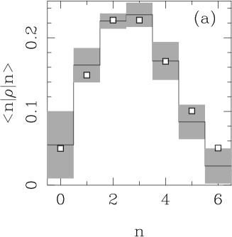
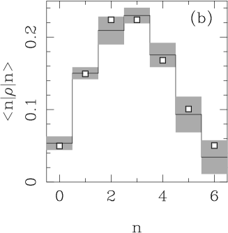
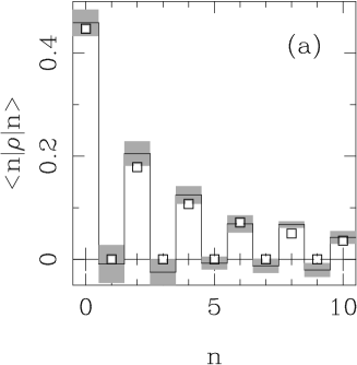
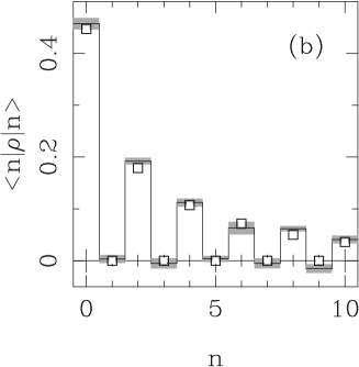
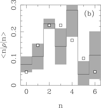
The adaptive method leads to a significant error reduction for detection of matrix elements of coherent states. Our results indicates that type-I null functions are the most effective, and that the larger is the amplitude of the coherent state, the larger the noise reduction. In Fig. 1 numerical results are presented for diagonal elements for intensity . In Fig. 1(a) the noise reduction is given versus the number of added type-I null functions. One can see that the noise reduction saturates for large , and better levels of reduction are achieved for smaller . In Fig. 1(b) the noise reduction is reported versus for . In Fig. 2 we report the results from a Monte Carlo experiment for , with optimization performed with null functions. The reduction of statistical errors for low values of is evident.
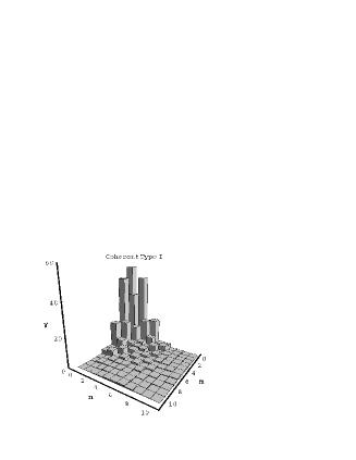
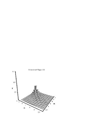
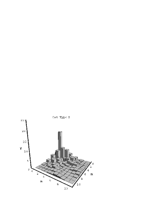
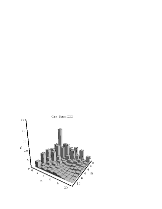
The noise reduction for the off-diagonal matrix elements behaves similarly to the diagonal ones, being more effective for low indices. In Fig. 3 the noise reduction versus and of the matrix element is plotted for a coherent state with , and for the three types of null functions. The type-I null functions are generally more effective, though not uniformly over all indices and .
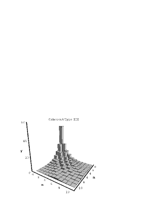
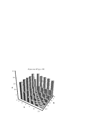
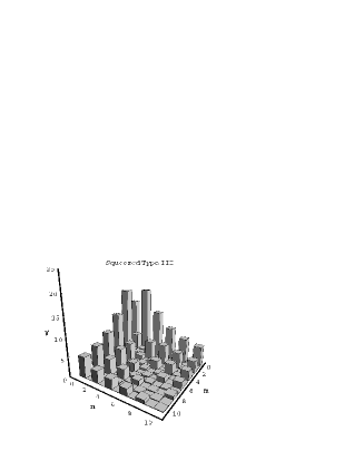
B Squeezed states and Schrödinger cat states
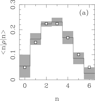
Results for squeezed states and ”cat” superposition of coherent states are presented in the same subsection, since they behave similarly. This is due to the fact that both states have phase-dependent features, that reflect in a similar odd-even oscillation in the photon number probability distribution. In Figs. 4 and 5 the noise reduction for both cases is plotted for the three types of null functions, for . From the plots it is apparent that type-II null functions are now the most effective ones, especially for off-diagonal matrix elements, though the same level of noise reduction for low and can also be obtained using type-I and type-III null functions. In Fig. 6 results from a Monte Carlo simulated adaptive tomography on a squeezed vacuum are reported for and . Matrix elements before and after optimization can be compared, showing the error reduction at work.
C Fock states
For Fock states the matrix is diagonal for all types of null functions, and therefore the optimization procedure just consists of the evaluation of the vector . The kernels for the matrix elements have the form , where has the parity of [2, 27]. This fact, together with the integral (14) makes straightforward to show that
| (33) |
namely no improvement should be expected for the precision of quantum tomography on Fock states.
IV Adaptive tomographic measurements of observables
The tomographic estimation of the ensemble average of a radiation operator can be obtained by averaging the kernel given in Eq. (2). However, Eq. (2) needs a procedure that exploits the null function equivalence, and is given in Ref. [28]. For this reason, for simplicity here we use the Richter formula [29], which expresses the kernels for the normally ordered moments as follows
| (34) |
being the Hermite polynomial of order . We apply the adaptive method to the tomographic detection of the most relevant observables: intensity, quadrature and complex field amplitude. The optimization method is here particularly useful, as the tomographic detection of these observables using the Richter kernel is very noisy [23, 30].
In contrast to the case of matrix elements given in Section III, here some analytical evaluations can be carried out. We consider measurements performed on coherent states, squeezed vacuum, Fock states and cat superposition of coherent states. It turns out that addition of just few null functions to the Richter kernels generally results in a large improvement of the tomographic precision, again with the exception of Fock states where no improvement can be obtained.
A Intensity
The tomographic detection of intensity is obtained by averaging the kernel
| (35) |
The vectors needed for the optimization procedure are given by
| (36) | |||||
| (39) | |||||
| (42) |
From Eqs. (39) and (42) it follows that only and are effective in reducing the variance. We solved analytically the optimization equations (23) for type-I null functions, and also in this case it turns out that for all the states here considered, only the single null function is needed, namely one has
| (43) |
The corresponding reduction of variance is easily obtained from Eq. (26), and is given by
| (44) |
Actually, can compensate the leading term of the variance of the original Richter kernel [23], which, in turn, is given by
| (45) |
This means that the variance of the optimized kernel becomes much closer to the intrinsic intensity fluctuations than the original noise . In order to appreciate such noise reduction we compare the two noise ratios
| (46) |
For coherent states we obtain
| (47) |
that is, from an asymptotically linearly increasing function of the ratio becomes a constant . Similar expressions are obtained for other kind of state: the noise ratio saturates to for either squeezed vacuum and cat states.
In Fig. 7 results from a Monte Carlo simulation of the tomographic measurement of intensity on coherent states show the noise reduction obtained when using the optimized kernel.
The noise reduction obtained by adding the single null function can be easily evaluated also for the generic diagonal moment , using the formula
| (48) |
which leads to
| (49) |
namely . We just mention that optimizing the kernel is useful to improve detection of the second order correlation function .
B Quadrature
The optimization procedure has been tested also on the kernel , corresponding to the measurement of the quadrature operator . Similarly to the intensity case, the type-II and type-III null functions do not play a role in improving precision, whereas type-I functions give in Eq. (23). In this way the optimization procedure can be carried analytically also in this case. The results indicate that for coherent states it is enough to add the first null function , whereas for squeezed vacuum and cat states only the odd-index functions contribute to noise reduction. In this case the main term is due to , whereas higher order functions improve the variances only by a few percent. For coherent states the variance reduction from is given by
| (50) |
which completely compensates the leading term in the variance of the original Richter kernel [23]
| (51) |
For squeezed vacuum and cat states the variance reduction due to is
| (52) |
Upon defining the noise ratio in analogy to Eq.(46)
| (53) |
from Eqs. (50) and (52) we get the constant for coherent states, independently on , whereas for squeezed vacuum and cat states the noise ratio saturates to . In Fig. 8 results from a simulated experiments of tomographic measurement of the quadrature on coherent states are shown for . There the histograms of the original Richter kernel and of the optimized kernel are compared. The optimized kernel has a sharper distribution, which is peaked at the mean value . For this reason, it is quite obvious that the optimized kernel gives a more precise determination of than the the original kernel .
C Field amplitude
The tomographic kernel for the measurement of the complex field amplitude is given by , and its fluctuations should be compared with those from the ideal measurement of , which could be achieved by ideal eight-port [32, 33, 34] or six-port [35, 36] homodyne detection. The optimization procedure depends on the choice for the definition of statistical error for a complex quantity. If one considers the real or the imaginary part separately, the procedure coincides with the optimization of the precision in independent measurements of two conjugated quadratures. On the other hand, in order to take into account both noises jointly, we minimize the quantity
| (54) |
corresponding to the average of noises for real and imaginary parts, namely the trace of the noise covariance matrix. Now, the equivalence class of kernel functions is written as follows
| (55) |
and being two independent sets of complex coefficients. The optimization procedure is similar to the real case, and is reduced to solving the two linear systems
| (56) |
where is given by
By inverting Eqs. (56), one obtains the noise reduction
| (57) |
Also in the present case it is sufficient to consider only type-I functions. The optimization vector is given by . Similarly to the case of the quadrature, the optimization procedure shows that for coherent states only is needed, whereas for squeezed vacuum and cat states only the odd-index functions contribute to noise reduction, and the main term comes from . In this way for coherent states one obtains
| (58) |
whereas for squeezed vacuum and cat states one has
| (59) |
Eqs. (58) and (59) should be compared with the noise-figure of the original Richter kernel
| (60) |
and with the intrinsic noise of a generalized measurement of the amplitude
| (61) |
The noise ratios thus equals for coherent states, whereas saturates to for both squeezed vacuum and cat states. Remarkably, for coherent states the heterodyne noise is reached, namely tomographic detection has ideal noise.
V Effects of systematic errors
Throughout this paper the tomographic kernels have been optimized by adding low order null functions. Higher order functions oscillate more rapidly. Since the method involves only the average of these functions on a small sample of data, fast oscillations in and higher power of would introduce more noise, and including too many null functions would increase the error instead of reducing it. In Fig. 9 an example of such pathology is given.
Another point that should be mentioned is that in the tomographic detection here considered the phase is a random parameter in . A discrete scanning by equally-spaced phases would introduce systematic errors [21, 31] that would mask the benefits from the optimization. Actually, for non-random uniform scanning, the null function has no effects when added to phase independent kernels, whereas the other null functions have a much reduced effect, and obviously do not eliminate the systematic error due to the finite mesh of the deterministic scanning.
VI Summary and Conclusions
In this paper we have presented an adaptive method to optimize tomographic kernels, improving the precision of the tomographic measurement. The method has been analyzed in detail for coherent states, Fock states, squeezed vacuum, and ”Schrödinger-cat” states. With the exception of Fock, states the method generally provides a sizeable reduction of statistical errors. For coherent states the improvement mainly concerns the small-index matrix elements, whereas for squeezed vacuum and cat states also far off-diagonal elements are improved.
The error reduction is much more significant for the measurement of intensity, quadrature and field amplitude, where for coherent states, squeezed vacuum, and cat states the ratio between tomographic noise and uncertainty of the considered observable saturates for increasing energy. In this case, we can definitely assert that quantum tomography is a quasi-ideal measurement, as it adds only a small amount of noise as compared to ideal detection.
Acknowledgments
We would thank Dirk -G. Welsch, Mohamed Dakna and Nicoletta Sterpi for useful discussions. M. G. A. Paris has been partly supported by the “Francesco Somaini” foundation. This work is part of the INFM contract PRA-1997-CAT.
REFERENCES
- [1] J. Mod. Opt. 44 (1997) special issue
- [2] For a review see: G. M. D’Ariano in Quantum Optics and Spectroscopy of Solids, ed. by A. S. Shumowsky and T. Hakiouglu (Kluwer Publishing – Amsterdam, 1997) p.175
- [3] For a more recent review see: D. -G. Welsch, W. Vogel, T. Opatrnỳ, Progr. Opt. Progr. Opt. (1999), in press.
- [4] D. F. McAlister, M. G. Raymer, Phys. Rev. A 55, R1609 (1997).
- [5] G. Breitenbach, S. Schiller, J. Mlynek, Nature 387 471 (1997).
- [6] M. Vasylìev, S-K. Choi, P. Kumar, G. M. D’Ariano, Opt. Lett. 23, 1393 (1998).
- [7] G. M. D’Ariano, M. Vasylìev, P. Kumar, Phys. Rev. A 58, 636 (1998).
- [8] G, M. D’Ariano, M. F. Sacchi, P. Kumar, Phys. Rev. A (1999), in press.
- [9] G. M. D’Ariano, L. Maccone, Phys. Rev. Lett. 80, 5465 (1998).
- [10] K. Vogel, H. Risken, Phys. Rev. A 40, 2847 (1989).
- [11] M. Beck, D. T. Smithey, and M. G. Raymer, Phys. Rev. A 48, R890 (1993).
- [12] G. M. D’Ariano, C. Macchiavello, M. G. A. Paris, Phys. Rev. A 50 4298 (1994).
- [13] G. M. D’Ariano, U. Leonhardt, H. Paul, Phys. Rev. A 52 1801 (1995).
- [14] K. Banaszek, K. Wódkiewicz, Phys. Rev. Lett. 76, 4344 (1996).
- [15] V. Bužek, G. Adam, G. Drobnỳ, Ann. Phys. (N.Y.) 245, 37 (1996).
- [16] M. G. A. Paris, Phys. Rev. A 53, 2658 (1996).
- [17] H. Kühn, D. -G. Welsch, W. Vogel, J. Mod. Opt. 41, 1607 (1998).
- [18] G. M. D’Ariano in Quantum Communication, Computing, and Measurement, ed. by O. Hirota, A. S. Holevo, C. M. Caves (Plenum Publishing, New York 1997) p. 253.
- [19] T. Opatrnỳ, D. -G. Welsch, Phys. Rev. A 55, 1462 (1997).
- [20] G. M. D’Ariano, C. Macchiavello, Phys. Rev. A 57 3131 (1998).
- [21] G. M. D’Ariano, C. Macchiavello, N. Sterpi, Quant. Semicl. Opt. 9, 929 (1997).
- [22] G. M. D’Ariano, C. Macchiavello, N. Sterpi, in Quantum Communication, Computing, and Measurement, ed. by G. M. D’Ariano, P. Kumar, O. Hirota (Plenum Publishing, New York 1999), in press.
- [23] G. M. D’Ariano, M. G. A. Paris, Phys. Lett. A 233 49 (1997).
- [24] T. Opatrny, M. Dakna, D.-G. Welsch, Phys. Rev. A 57 2129 (1998).
- [25] G. M. D’Ariano, M. G. A. Paris, Acta Phys. Slov. 48 (1998).
- [26] R. M. Wilcox, J. Math. Phys. 8, 962 (1967).
- [27] U. Leonhardt, M. Munroe, T. Kiss, Th. Richter, M. G. Raymer, Opt. Comm. 127 144 (1996).
- [28] G. M. D’Ariano in Quantum Communication, Computing, and Measurement, ed. by G. M. D’Ariano, P. Kumar, O. Hirota (Plenum Publishing, New York 1999), in press.
- [29] Th. Richter, Phys. Lett. A 221 327 (1996).
- [30] G. M. D’Ariano, M. G. A. Paris, Acta Phys. Slov. 47 281 (1997).
- [31] U. Leonhardt, M.Munroe, Phys. Rev. A 54 3682 (1996).
- [32] N. G. Walker, J. Mod. Opt. 34, 15 (1987).
- [33] Y. Lay, H. A. Haus, Quantum Opt. 1, 99 (1989).
- [34] G. M. D’Ariano, M. G. A. Paris, Phys. Rev. 49 3022 (1994).
- [35] A. Zucchetti, W. Vogel, D.-G. Welsch, Phys. Rev. A54 856 (1996)
- [36] M. G. A. Paris, A. Chizhov, O. Steuernagel, Opt. Comm. 134, 117 (1997).
 |
 |
 |
 |
 |
 |
 |
 |
 |
 |
 |
 |
 |
 |
 |
 |
 |
 |
 |
 |
 |
| l | 0 | 1 | 2 | 3 | 4 | 5 | 6 | 7 | .. |
|---|---|---|---|---|---|---|---|---|---|
| k+n | 0 | 1 | 1 | 2 | 2 | 2 | 3 | 3 | .. |
| k | 0 | 1 | 0 | 2 | 1 | 0 | 3 | 2 | .. |
| n | 0 | 0 | 1 | 0 | 1 | 2 | 0 | 1 | .. |