Heterodyne and adaptive phase measurements on states of fixed mean photon number

Abstract

The standard technique for measuring the phase of a single-mode field is heterodyne detection. Such a measurement may have an uncertainty far above the intrinsic quantum phase uncertainty of the state. Recently it has been shown [H. M. Wiseman and R. B. Killip, Phys. Rev. A 57, 2169 (1998)] that an adaptive technique introduces far less excess noise. Here we quantify this difference by an exact numerical calculation of the minimum measured phase variance for the various schemes, optimized over states with a fixed mean photon number. We also analytically derive the asymptotics for these variances. For the case of heterodyne detection our results disagree with the power law claimed by D’Ariano and Paris [Phys. Rev. A 49, 3022 (1994)].

I Introduction

It is well known that it is not possible to make quantum-limited measurements of the phase of an electromagnetic field using linear optics and photodetectors fullquan . The standard method of making a (non-quantum-limited) phase measurement is by heterodyne detection. Heterodyne detection involves combining the field to be measured with a much stronger local oscillator field which has a frequency detuned by a small amount $\Delta$, and measuring the intensity of the resultant field. In a typical experimental implementation, the mode to be measured is passed through a 50/50 beam splitter, in order to combine it with the local oscillator. The difference photocurrent from the two output ports of the beam splitter yields a measurement of the phase quadrature $X_{\Phi}=ae^{-i\Phi}+a^{\dagger}e^{i\Phi}$, where $a$ is the annihilation operator of the mode to be measured and $\Phi$ is the phase of the local oscillator. In heterodyne measurement the detuning $\Delta$ is typically chosen to be large enough that the phase of the local oscillator cycles many times over the course of the measurement, so as to measure all quadratures with equal accuracy.

In a heterodyne phase measurement of a coherent state of amplitude $\alpha$, the variance in the measured phase $\phi$ scales as semiclass

$$V_{\rm het}(\phi)=\frac{1}{2|\alpha|^{2}}.$$ (1)

This is twice the intrinsic uncertainty of the coherent state. An improved phase measurement can be made if one has an initial estimate of the phase. Then one would choose the local oscillator phase $\Phi$ to be equal to $\varphi+\pi/2$, where $\varphi$ is the initial estimated phase of the field to be measured. This is known as homodyne detection. If the phase is unknown before the measurement, then one can still apply this idea by adjusting the phase of the local oscillator during the course of the measurement based on an estimate of the phase from the measurement results so far.

These adaptive phase measurements have been discussed in a series of papers by Wiseman Wise95 and Wiseman and Killip semiclass ; fullquan . In Ref. semiclass it was shown that via adaptive measurements of a coherent state one can obtain a phase uncertainty of

$$V_{\rm adapt}(\phi)=\frac{1}{4\alpha^{2}}+\frac{1}{8\alpha^{3}}.$$ (2)

Here we have taken the coherent amplitude $\alpha$ to be real. The first term above is the intrinsic uncertainty of the coherent state, and the second term is the extra phase uncertainty introduced by the phase measurement. This result implies that even though there is not much improvement in using adaptive phase measurements on coherent states, if the input state has reduced phase uncertainty then adaptive measurements will produce a phase measurement with far less uncertainty than a heterodyne measurement.

To better quantify the improvement offered by adaptive measurements, it is necessary to consider the variance of states that have been optimized for minimum phase variance under various measurement schemes. There must be a constraint placed on optimizing states, otherwise a phase eigenstate will be obtained. The two main ways in which to constrain the states are by truncating the photon number and by fixing the mean photon number. The case of truncated photon number was considered analytically in Ref. semiclass , and numerically in Ref. fullquan . The case of a fixed mean photon number is determined analytically in Sec. IV below.

General optimized states are difficult to work with, as they cannot be generated experimentally. Also, in numerical integration of the stochastic differential equations arising from the various measurement schemes (to be considered in future work), calculations must be performed on the entire state for general optimized states. This becomes prohibitively time consuming for large photon numbers. Squeezed states are far more practical, as they are routinely generated experimentally, and in numerical integration only the two squeezing parameters need be considered. The theory for optimized squeezed states is considered in Sec. V. The analytical results for both general states and squeezed states are tested numerically in Sec. VI, and the implications discussed in Sec. VII.

II POMs and phase measurements

In quantum-mechanical systems, the most general way of obtaining the probability of some measurement result $E$ is by the expectation value of an operator $F(E)$, i.e.,

$$P(E)={\rm Tr}[\rho F(E)],$$ (3)

where $\rho$ is the state matrix for the system. If the set of all possible measurement results is $\Omega$, it is evident that $P(\Omega)=1$ for all $\rho$, which implies that $F(\Omega)=1$. Thus $F(E)$ can be called a probability operator, and the mapping $E\mapsto F$ defines a probability operator measure (POM) on $\Omega$ Dav76 ; Hel76 .

For phase measurements on a single-mode field, the general form of the POM is semiclass

$$F(\phi)=\frac{1}{2\pi}\sum_{n,m=0}^{\infty}|{m}\rangle\langle{n}|e^{i\phi(m-n)}H_{mn},$$ (4)

where $H$ is a positive-semidefinite symmetric matrix with all entries positive, and $|{m}\rangle$ is a number state of the field. In this case $\Omega=[0,2\pi)$ and the completeness relation is

$$\int_{0}^{2\pi}d\phi F(\phi)={\rm diag}[H_{00},H_{11},H_{22},\ldots]=1.$$ (5)

For ideal phase measurements all elements of the $H$ matrix are equal to 1, whereas for physical measurements the off-diagonal elements will generally be less than 1 semiclass .

The accuracy of phase measurements can be quantified in a number of ways Hol84 ; Opatrny which agree in the limit of small phase variance provided the phase distribution is narrowly peaked (as it will be in the examples we consider). When the mean phase is zero it is easiest to define the phase variance as

$$V(\phi)=2-2\left\langle{\cos\phi}\right\rangle=2(1-{\rm Re}\langle e^{i\phi}\rangle).$$ (6)

If we evaluate $\langle e^{i\phi}\rangle$ using Eq. (4) for an arbitrary pure quantum state $|{\psi}\rangle$, we obtain

$$\langle{e^{i\phi}}\rangle=\sum_{m=0}^{\infty}\langle{\psi}|{m}\rangle\langle{m+1}|{\psi}\rangle H_{m,m+1}.$$ (7)

Therefore, the phase variance only depends on the off-diagonal elements $H_{m,m+1}$, and we may characterize a phase measurement by the vector

$$h(m)=1-H_{m,m+1}.$$ (8)

For most phase measurements, we have for large photon numbers semiclass

$$h(m)\approx cm^{-p}.$$ (9)

Then for states with a reasonably well-defined mean photon number $\bar{n}$ the total phase variance is given approximately by semiclass

$$V(\phi)\approx V_{\rm intrinsic}(\phi)+2h(\bar{n}),$$ (10)

where $V_{\rm intrinsic}(\phi)$ is the phase variance which would result from an ideal or canonical measurement of the phase Lon27 ; LeoVacBohPau95 . Evidently $h(\bar{n})$ is a measure of the excess phase noise introduced by the measurement, and it would be desirable to make this as small as possible.

III Adaptive Measurements

In a real optical experiment one cannot directly measure the phase, but would rather estimate it from a photocurrent record. Here the photocurrent would be derived by combining the mode to be measured with a local oscillator via a 50/50 beam splitter. Such measurements have been called dyne measurements, as they include homodyne and heterodyne as well as adaptive measurements fullquan . The signal of interest is the difference between the photocurrents at the two ports, which we define by

$$I(t)=\lim_{\delta t\rightarrow 0}\lim_{\beta\rightarrow\infty}\frac{\delta N_{+}(t)-\delta N_{-}(t)}{\beta\delta t},$$ (11)

where $\delta N_{\pm}$ are the increments in the photocounts at the two detectors in the interval $[t,t+\delta)$ and $\beta$ is the amplitude of the local oscillator.

Say the mode to be measured has an (assumed positive) envelope $u(t)$ normalized such that $\int_{0}^{\infty}u(t)dt=1$. For simplicity, define a scaled time $v$ by

$$v=\int_{0}^{t}u(s)ds,$$ (12)

so that $v\in[0,1)$. Then it turns out that at time $v$ there are two sufficient statistics for the measurement record:

$$A_{v}=\int_{0}^{v}I(u)e^{i\Phi(u)}du,~{}~{}~{}B_{v}=-\int_{0}^{v}e^{2i\Phi(u)}du.$$ (13)

These are sufficient statistics in the sense that the POM for the measurement is a function of $A_{v}$ and $B_{v}$ only Wise96 . This means that the best estimate for the phase at time $v$ need depend on the measurement record only through the complex numbers $A_{v}$ and $B_{v}$.

Consider the simple case where the mode is initially in a coherent state $|{\alpha}\rangle$. We can then take the limits in Eq. (11) to obtain

$$I(v)=2\text{Re}(\alpha e^{-i\Phi(v)})+\xi(v),$$ (14)

where $\xi(v)=dW(v)/dv$ is the shot noise semiclass . From this we can evaluate $A_{v}$ as

$$A_{v}=\alpha v-\alpha^{*}B_{v}+\int_{0}^{v}e^{2i\Phi(u)}dW(u).$$ (15)

If one ignores the final term (which has zero expectation value), it is easy to see that $\arg\alpha=\arg(vA_{v}+B_{v}A_{v}^{*})$. Other arguments Wise96 suggest that this is generally the best estimate for the phase at time $v$. If $B_{v}$ is small (as it is in heterodyne detection), this can be approximated by $\arg A_{v}$. The adaptive phase measurements that were analyzed in Refs. semiclass and fullquan use $\arg A_{v}$ as the phase estimate during the measurement, setting

$$\Phi(v)=\arg A_{v}+\pi/2.$$ (16)

The main motivations for this choice are that it gives a feedback algorithm which would be easy to implement experimentally, and that it is mathematically tractable.

If the phase estimate $\arg A$ is used at the end of the adaptive measurement, the resultant phase measurement is actually worse than a heterodyne phase measurement. This phase measurement is called an adaptive mark I phase measurement, and it was found semiclass that

$$h_{\rm I}(m)\approx\frac{1}{8m^{1/2}},$$ (17)

which compares with

$$h_{\rm het}(m)\approx\frac{1}{8m}.$$ (18)

If the phase estimate $\arg(A+BA^{*})$ is used at the end of the phase measurement, a far better phase measurement is obtained. This phase measurement is called an adaptive mark II phase measurement, and yields semiclass

$$h_{\rm II}(m)\approx\frac{1}{16m^{3/2}},$$ (19)

which is considerably better than the standard (heterodyne) result. However, as noted in Sec. I, this dramatic improvement can only be seen if one starts with a state having intrinsic phase variance much less than that of a coherent state, for which $V_{\rm intrinsic}=2h_{\rm het}(\alpha^{2})$.

In practice, imperfections in the equipment can introduce phase uncertainties that scale as $\bar{n}^{-1}$ semiclass . The main problems are inefficient detectors and time delays. From Ref. semiclass , the extra phase variance introduced by inefficient detectors is

$$\delta V_{\rm II}(\phi)=\frac{1-\eta}{4\eta\overline{n}},$$ (20)

where $\eta$ is the efficiency. Again from Ref. semiclass the extra phase variance introduced by a time delay $\delta v$ is

$$\delta V_{\rm II}(\phi)\sim\frac{\delta v}{\bar{n}}.$$ (21)

This means that when the photon number is sufficiently large, above $(1-\eta)^{-2}$ or $(\delta v)^{-2}$, the introduced phase variance will always scale as $\overline{n}^{-1}$. Nevertheless, adaptive measurements will always give more accurate results than heterodyne measurements, and it is of interest to know how accurate phase measurements can be made in principle, since future technological advances may greatly reduce the problems of detector inefficiencies and time delays.

IV General optimized states

The fairest way to compare different phase measurement schemes is to consider the phase variances for states optimized for minimum total phase variance for the particular measurement under consideration. The two alternative constraints which can be put on the optimization are (i) an upper limit on the photon number, or (ii) a fixed mean photon number. The case where an upper limit $N$ is put on the photon number was considered in Refs. semiclass ; fullquan , where the minimum phase variance was found to be

$$V(\phi)\approx 2cN^{-p}+(-z_{1})(2cp)^{2/3}N^{-2(1+p)/3},$$ (22)

where $z_{1}$ is the first zero of the Airy function, and is equal to approximately $-2.338$.

Here we will be considering the case of fixed mean photon number. Let us take the phase to be zero and use the operator for the phase variance

$$\hat{S} =2-2\widehat{\cos{\phi}}$$ (23a)

$$=2-\sum_{m=0}^{\infty}\left[1-h(m)\right]\left(|{m}\rangle\langle{m+1}|+{\rm H.c.}\right).$$ (23b)

In order to optimize for minimum phase variance with a fixed mean photon number, we use the method of undetermined multipliers. We have two constraints on the state: that the mean photon number is fixed and that the state is normalized. This then gives us an equation with two undetermined multipliers

$$(\hat{S}+\mu\hat{N})|{\psi}\rangle=\nu|{\psi}\rangle.$$ (24)

We solve this as an eigenvalue equation for $\nu$ with a fixed value of $\mu$, and the eigenstate corresponding to the minimum eigenvalue is the optimized state. The mean photon number can then be found from the state. The mean photon number can be varied by varying $\mu$, but cannot be easily predicted from $\mu$.

This method was used by Summy and Pegg meanN to find states with fixed mean photon number optimized for minimum intrinsic phase variance. They found that the minimum phase uncertainty was approximately

$$\left\langle{(\Delta\phi)^{2}}\right\rangle_{\rm intrinsic}^{\rm min}=\frac{C}{(\bar{n}+\epsilon)^{2}},$$ (25)

where $C\approx 1.88$ and $\epsilon\approx 0.86$. Therefore, the minimum intrinsic phase variance scales as $\bar{n}^{-2}$.

If the state is expressed in the number states basis

$$|{\psi}\rangle=\sum_{n=0}^{\infty}b_{n}|{n}\rangle,$$ (26)

then in terms of $b_{n}$, Eq. (24) becomes

$$2b_{n}-\left[1-h(n)\right]\left(b_{n+1}+b_{n-1}\right)=\left(\nu-\mu n\right)b_{n}.$$ (27)

In the case of very large mean photon number, we can use a continuous approximation

$$2h(x)y-[1-h(x)]\frac{d^{2}y}{dx^{2}}=\left(\nu-\mu x\right)y,$$ (28)

where we are taking $x=n$ and $y(x)=b_{n}$. For large $n$, $\left[1-h(n)\right]\approx 1$, so

$$-\frac{d^{2}y}{dx^{2}}+y\left[2h(x)-\nu+\mu x\right]\approx 0.$$ (29)

Now define

$$f(x)=2h(x)-\nu+\mu x.$$ (30)

Then, expanding $f(x)$ in a Taylor series around

$$x_{0}=(\mu/2cp)^{-1/(p+1)},$$ (31)

we find

$$f(x_{0}) =2h(x_{0})-\nu+\mu x_{0},$$ (32a)

$$f^{\prime}(x_{0}) =2h^{\prime}(x_{0})+\mu=-2cpx_{0}^{-p-1}+\mu=0,$$ (32b)

$$f^{\prime\prime}(x_{0}) =2h^{\prime\prime}(x_{0})=2cp(p+1)x_{0}^{-p-2},$$ (32c)

$$f^{\prime\prime\prime}(x_{0}) =-2cp(p+1)(p+2)x_{0}^{-p-3}.$$ (32d)

This technique requires that the number distribution has its maximum near $x_{0}$, which will be justified below.

Using the Taylor series for $f(x)$, and defining $f_{0}=f(x_{0})$, $f_{2}=f^{\prime\prime}(x_{0})/2$, and $f_{3}=f^{\prime\prime\prime}(x_{0})/6$, the differential equation (29) becomes

$$-\frac{d^{2}y}{dx^{2}}+[f_{2}(x-x_{0})^{2}+{f_{3}}(x-x_{0})^{3}]y\approx-f_{0}y.$$ (33)

Note that $-f_{0}=\nu-[2h(x_{0})+\mu x_{0}]$, so the above equation is equivalent to solving Eq. (24) as an eigenvalue equation for $\nu$ with a fixed value of $\mu$. Now Eq. (33) is equivalent to the time-independent Schrödinger equation with energy eigenvalue $E=-f_{0}$ for a perturbed harmonic Hamiltonian $\hat{H}=\hat{H}_{0}+\hat{H}_{1}$, where

$$\hat{H}_{0} =\sqrt{f_{2}}\left[-\frac{d^{2}}{d\xi^{2}}+\xi^{2}\right],$$ (34a)

$$\hat{H}_{1} =b\xi^{3},$$ (34b)

where

$$b =-\frac{p+2}{3}\left[cp(p+1)\right]^{1/4}x_{0}^{-p/4-3/2},$$ (35a)

$$\xi =f_{2}^{1/4}(x-x_{0}).$$ (35b)

The unperturbed solution is

$$y_{j}^{(0)}(\xi)=(\pi^{1/2}2^{j}j!)^{-1/2}\exp(-\xi^{2}/2)H_{j}(\xi),$$ (36)

where $H_{j}$ are Hermite polynomials. This solution is only valid for $\sqrt{f_{2}}x_{0}^{2}\gg 1$, which requires that $p<2$ in addition to $x_{0}\gg 1$. The energy eigenvalues are

$$E_{j}^{(0)}=(2j+1)\sqrt{f_{2}}.$$ (37)

The lowest energy eigenvalue $E_{0}$ and corresponding eigenstate $y_{0}$ will minimize $\nu$ and therefore minimize $\langle\hat{S}\rangle$. From perturbation theory they can be expressed as

$$E_{0} \approx E_{0}^{(0)}+\langle{0}|\hat{H}_{1}|{0}\rangle-\frac{b^{2}}{2\sqrt{f_{2}}}\sum_{k=1}^{\infty}\frac{\left|\langle{k}|\xi^{3}|{0}\rangle\right|^{2}}{k},$$ (38a)

$$y_{0} \approx y_{0}^{(0)}-\frac{b}{2\sqrt{f_{2}}}\sum_{k=1}^{\infty}\frac{\langle{k}|\xi^{3}|{0}\rangle}{k}y_{k}^{(0)},$$ (38b)

where $|{j}\rangle$ is the state corresponding to $y_{j}^{(0)}(\xi)$. Now it is easily shown using the properties of Hermite polynomials that the only nonzero terms are $\langle{1}|\xi^{3}|{0}\rangle=3/{2\sqrt{2}}$ and $\langle{3}|\xi^{3}|{0}\rangle={\sqrt{3}}/2$. This then gives the lowest energy eigenvalue and eigenstate as

$$E_{0} \approx E_{0}^{(0)}-b^{2}\frac{11}{16}f_{2}^{-1/2},$$ (39a)

$$y_{0} \approx y_{0}^{(0)}-\frac{b}{4\sqrt{2f_{2}}}\left[3y_{1}^{(0)}+\sqrt{\frac{2}{3}}y_{3}^{(0)}\right].$$ (39b)

Now we can use these expressions to find the mean photon number as

$$\bar{n} =\left\langle{x}\right\rangle=\int y_{0}(\xi)(x_{0}+f_{2}^{-1/4}\xi)y_{0}(\xi)d\xi$$ (40a)

$$\approx x_{0}+\frac{p+2}{4\sqrt{cp(p+1)}}x_{0}^{p/2}.$$ (40b)

As we are assuming $p<2$,

$$x_{0}\approx\bar{n}\left[1-\frac{p+2}{4\sqrt{cp(p+1)}}\bar{n}^{p/2-1}\right],$$ (41)

so that the mean photon number is close to $x_{0}$, justifying the previous expansion around $x_{0}$. Now we can find the minimum phase variance using

$$\langle\hat{S}\rangle_{\rm min}=(\nu-\mu\bar{n})_{\rm min},$$ (42)

and $\nu=-f_{0}+2h(x_{0})+\mu x_{0}$, $\mu=2cpx_{0}^{-p-1}$, and $f_{0}=-E_{0}$. We obtain the first two terms as

$$\langle\hat{S}\rangle_{\rm min}\approx 2c\bar{n}^{-p}+\sqrt{cp(p+1)}\bar{n}^{-p/2-1}.$$ (43)

Note that the first term here is the same as the result when an upper limit is put on the photon number, but the second term scales as a different power of $\bar{n}$.

A particular case of interest is heterodyne detection, for which we find

$$\langle\hat{S}\rangle^{\rm min}_{\rm het}\approx\frac{1}{4\bar{n}}+\frac{1}{2\bar{n}^{3/2}}.$$ (44)

This is interesting because it differs radically from the result claimed by D’Ariano and Paris DArPar94 of

$$\langle(\Delta\phi)^{2}\rangle_{\rm het}^{\rm min}=\frac{1.00\pm 0.02}{\bar{n}^{1.30\pm 0.02}}.$$ (45)

As the quoted errors suggest, this result was obtained entirely numerically, in contrast to our analytical result. In Sec. VI we present our own numerical results and show that our analytical result is a far better fit than the power law of D’Ariano and Paris.

V Optimized squeezed states

As an alternative to considering general optimized states, we can consider optimized squeezed states. There are three reasons for this:

(1) Squeezed states are relatively easily generated in the laboratory, whereas there is no known way of producing general optimized states experimentally.

(2) Squeezed states can be treated numerically far more easily than general optimized states.

(3) It has been found numerically (see Sec. VI) that the phase uncertainties of optimized squeezed states are very close to those of optimized general states, and a partial theoretical explanation can be obtained by the following analysis.

Squeezed states optimized for minimum intrinsic phase variance were previously considered by Collett Collett93 , who found that the minimum phase uncertainty was approximately given by

$$\langle(\Delta\phi)^{2}\rangle_{\rm intrinsic}\approx\frac{\ln(\bar{n})+\Delta}{4\bar{n}^{2}},$$ (46)

where $\Delta=\frac{3}{2}+2\ln 2-\frac{1}{4}\ln(2\pi)$. The scaling of optimized squeezed states is therefore worse than the scaling of optimized general states when we consider intrinsic phase variance. The difference is only a factor of $\ln\bar{n}$, however.

We consider squeezed states of the form

$$|{\alpha,\zeta}\rangle=\exp(\alpha a^{\dagger}-\alpha^{*}a)\exp[(\zeta^{*}a^{2}-\zeta a^{\dagger 2})/2]|{0}\rangle.$$ (47)

Now we will take the phase to be 0, so $\alpha$ is real. Phase squeezed states have $\zeta$ real and negative, so we can take $\zeta$ to be real. Then using the definition of phase uncertainty in Eq. (6) gives

$$\langle(\Delta\phi)^{2}\rangle =2-2\sum_{n=0}^{\infty}\langle{\alpha,\zeta}|{n}\rangle\langle{n+1}|{\alpha,\zeta}\rangle$$

$$~{}~{}~{}+2\sum_{n=0}^{\infty}h(n)\langle{\alpha,\zeta}|{n}\rangle\langle{n+1}|{\alpha,\zeta}\rangle.$$ (48)

In estimating the intrinsic phase uncertainty, Collett Collett93 found the first two terms on the right-hand side to be approximately $(n_{0}+1)/4\overline{n}^{2}+2\mathop{\rm erfc}(\sqrt{2n_{0}})$, where $n_{0}=\overline{n}e^{2\zeta}$. We therefore only have to determine an expression for the third term. Using $h(n)\approx cn^{-p}$ as usual, the result we require is derived in the Appendix:

$$\sum_{n=0}^{\infty}n^{-p}\langle{\alpha,\zeta}|{n}\rangle\langle{n+1}|{\alpha,\zeta}\rangle\approx\overline{n}^{-p}\left[1+\frac{p(p+1)}{2n_{0}}\right].$$ (49)

The phase uncertainty is therefore given by

$$\langle(\Delta\phi)^{2}\rangle\approx\frac{n_{0}\!+\!1}{4\overline{n}^{2}}+2\mathop{\rm erfc}(\sqrt{2n_{0}})+2c\overline{n}^{-p}\!\left[1\!+\!\frac{p(p+1)}{2n_{0}}\right]\!.$$

Taking the derivative with respect to $n_{0}$ gives

$$\frac{\partial\langle(\Delta\phi)^{2}\rangle}{\partial n_{0}}\approx\frac{1}{4\overline{n}^{2}}-\sqrt{\frac{8}{\pi n_{0}}}e^{-2n_{0}}+2c\overline{n}^{-p}\left[\frac{-p(p+1)}{2n_{0}^{2}}\right].$$ (51)

As the second term falls exponentially with $n_{0}$, it can be omitted. Then we find that the minimum phase variance occurs for

$$n_{0}\approx 2\sqrt{cp(p+1)}\overline{n}^{1-p/2}.$$ (52)

Thus we find that $n_{0}\propto\bar{n}^{1-p/2}$, as was used in the Appendix. Substituting this result into Eq. (LABEL:phunc1) gives

$$\langle(\Delta\phi)^{2}\rangle_{\rm min}\approx 2c\overline{n}^{-p}+\sqrt{cp(p+1)}\overline{n}^{-p/2-1}.$$ (53)

We therefore obtain exactly the same first two terms for the phase uncertainty when considering squeezed states as we do when considering general states.

VI Numerical results

The analytic results from Secs. IV and V have been verified numerically by calculating the optimized states for heterodyne measurements and adaptive mark I and II measurements. For moderate mean photon numbers the calculations were exact, except in that a cutoff at large photon numbers was used.

For larger photon numbers an additional approximation was that asymptotic expressions for $h(m)$ were used. For heterodyne measurements there is an exact expression for $h(m)$ fullquan ,

$$h_{\rm het}(m)=1-\frac{\Gamma\left(m+3/2\right)}{\sqrt{\Gamma\left(m+1\right)\Gamma\left(m+2\right)}}.$$ (54)

This form of the equation is very inconvenient for use in numerical work due to roundoff error. It is more convenient to use the asymptotic expansion. From the asymptotic expansion of $\ln\Gamma(m)$ Erdelyi53 it is simple to find an expansion of $h_{\rm het}(m)$ in powers of $1/(m+1)$ to as many terms as required. The first few terms are given by

$$h_{\rm het}(m)=\frac{1}{8(m+1)}-\frac{1}{2^{7}(m+1)^{2}}+O\left(m^{-3}\right).$$ (55)

An expansion up to 12th order was used to determine $h_{\rm het}(m)$. This expansion was found to be more accurate than using the formula directly for values of $m{\gtrsim}12$.

For adaptive mark I and adaptive mark II measurements, $h(m)$ can be determined using methods discussed in Ref. fullquan . For the mark I case $h_{\rm I}(m)$ was determined exactly up to $m=3000$. Further values were extrapolated by fitting an asymptotic expansion to the results below 3000. The first three terms of the asymptotic expansion used were

$$h_{\rm I}(m)=\frac{1}{8m^{1/2}}-\frac{0.101562}{m}-\frac{0.0508}{m^{3/2}}+O(m^{-2}).$$ (56)

The uncertainties in these numbers were estimated using various methods of fitting, and are indicated by the number of significant figures quoted.

For the mark II case $h_{\rm II}(m)$ was determined exactly up to $m=1000$. Fitting techniques did not consistently give any higher-order terms than that obtained by the semiclassical theory, so for $m>1000$ the formula $h_{\rm II}(m)=\frac{1}{16}m^{-3/2}$ was used.

For very large mean photon numbers ${\gtrsim}10^{5}$, it was not feasible to solve the exact eigenvalue problem, but an approximate solution was obtained by using the continuous approximation of the eigenvalue problem and discretizing it. In order to reduce the number of intervals required in the discretized equation, the equation was solved for three different numbers of intervals. The result for the continuous case was then estimated by projecting to zero step size, assuming the error is quadratic in the step size. For optimized squeezed states the full calculation was performed up to a mean photon number of about $10^{6}$, beyond which roundoff error became too severe.

The results of the numerical calculation for the general optimized states are shown in Fig. 1, along with the analytical results obtained in Sec. IV and the power law of Eq. (45) published by D’Ariano and Paris DArPar94 . It is seen that the results for heterodyne measurements agree reasonably well with the power law of D’Ariano and Paris for moderate photon numbers (up to about 100). Above this, however, the agreement is extremely poor. This is presumably due to the fact that the numerical data used by D’Ariano and Paris seems to have been limited to maximum photon numbers only of order 100. In contrast, our analytical result agrees very well for mean photon numbers above about 100. The analytical result also agrees well with the numerical results for the adaptive mark I and II measurements.

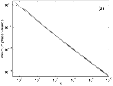
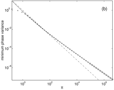
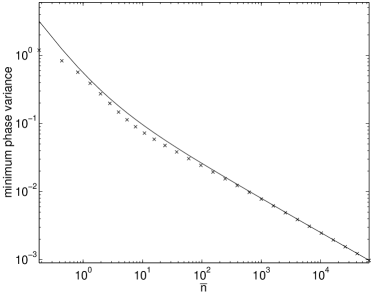
Figure 1: Plot of the phase variance for general optimized states via complete eigenvalue solution (crosses) and continuous approximation (circles) vs mean photon number $\bar{n}$. The asymptotic analytical expression from Sec. IV is also plotted (continuous lines). The three phase detection schemes are (a) mark II adaptive, (b) heterodyne, and (c) mark I adaptive. The power law claimed by D’Ariano and Paris for heterodyne detection is also plotted in (b) (dash-dot line).

On the log-log plot of the phase variance it is extremely difficult to discriminate between different phase variances unless the difference is greater than a factor of 2. Therefore, in Fig. 2 we plot the parameter $z$, defined by

$$z=(\langle(\Delta\phi)^{2}\rangle_{\rm min}-2c\bar{n}^{-p})\bar{n}^{p/2+1}.$$ (57)

From the above analysis this parameter should converge to $\sqrt{cp(p+1)}$ for large $\bar{n}$. The $z$ parameter is plotted for optimized general states and optimized squeezed states for the cases of mark II, heterodyne and mark I measurements in Figs. 2(a), 2(b), and 2(c), respectively.

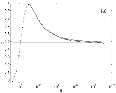
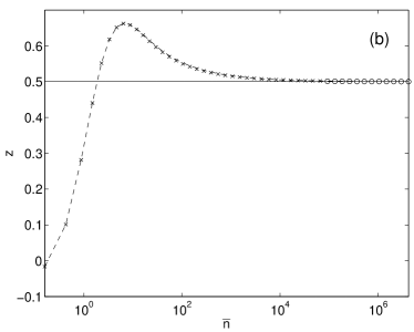
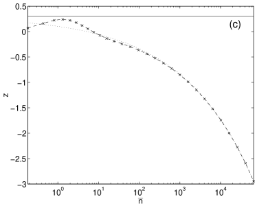
Figure 2: Plot of $z$ parameter from Eq. (57) for general optimized states via the complete eigenvalue solution (crosses) and continuous approximation (circles), and optimized squeezed states (dashed lines), vs mean photon number $\bar{n}$. The theoretical asymptotic value of $\sqrt{cp(p+1)}$ is shown as the continuous horizontal lines. The results shown are for mark II adaptive phase measurements in (a), heterodyne measurements in (b), and mark I adaptive measurements in (c). The predicted $z$ for the mark I case taking into account the second term for $h_{\rm I}(m)$ is also plotted in (c) (dotted line).

In the adaptive mark II and heterodyne results in Fig. 2(a) and 2(b), we can see that the results using the full eigenvalue solution match up very well with the continuous approximation results, demonstrating the accuracy of this technique. In addition, the squeezed-state results are extremely close to the general optimized state results, far closer than indicated by the first two terms derived above. Also note that in Fig. 2(a) the results do not agree closely (within 1%) with the asymptotic value until $\bar{n}>10^{8}$, whereas the heterodyne results converge at a much lower photon number, with good agreement for $\overline{n}{\approx}10^{4}$.

In the adaptive mark I results in Fig. 2(c), there is again good agreement between the squeezed-state results and the general optimized state results. However these results do not approach the asymptotic value at all in this case. The reason for this is that there is a higher-order term in $h_{\rm I}(m)$ which is of order $m^{-1}$, as shown in Eq. (56). This term is of lower order than the second term in the expansion (43) of the phase variance, which is of order $m^{-5/4}$. If the higher-order term in $h_{\rm I}(m)$ is taken into account in predicting the asymptotic value, then there is good agreement with the numerical results.

Although the adaptive mark I scheme has the poorest performance for large mean photon numbers, note from Fig. 1 that for small mean photon numbers (of order unity) it is actually the best scheme, having the smallest minimum phase variance. This is to be expected from the results of previous work Wise95 ; fullquan , showing that for a maximum photon number of 1, the adaptive mark I scheme is actually the best possible.

The significance of these results is, first, that the two terms given by the theory for optimized general and squeezed states are correct, and, second, that the phase uncertainties of optimized squeezed states are extremely close to those for optimized general states. This result is of great importance, as it means that in numerical and experimental work squeezed states can be used rather than general states.

This is an advantage in numerical work because only the squeezing parameters need be considered, rather than the entire state. This means that, for example, a numerical evaluation of different feedback schemes is feasible, and this work is being carried out now. In experimental work it is an advantage because squeezed states can be produced experimentally, whereas arbitrary states cannot. This means that it is possible to produce states experimentally that are very close to optimized for the different measurement schemes.

VII conclusion

We have derived asymptotic analytical expressions for the minimum phase variances obtainable under various detection schemes, for states constrained by their mean photon number. The detection schemes considered were heterodyne detection (a standard scheme), and two single-shot adaptive schemes (first proposed in Refs. Wise95 ; semiclass ), called mark I and mark II. Numerical results confirm the correctness of the first two terms in the asymptotic expansion, except in one case (adaptive mark I), where the second term was not expected to be correct. Furthermore, analytical and numerical results show that essentially the same results may be obtained using squeezed states, rather than completely general states. This is an important result from both theoretical and experimental standpoints.

As expected, the minimum phase variance for adaptive mark II measurements was much smaller than that for the standard technique of heterodyne detection, for large mean photon number $\overline{n}$. In particular, the leading term in the former scaled as $\overline{n}^{-3/2}$ compared to $\overline{n}^{-1}$ in the latter. The claim by D’Ariano and Paris DArPar94 that the heterodyne phase variance scaled as $\overline{n}^{-1.30}$ (or, as stated in their abstract, $\overline{n}^{-4/3}$) was proven wrong. This reinforces the position of adaptive mark II phase measurements as the best known phase measurement scheme.

In Ref. fullquan it was shown that a lower bound for the phase uncertainty introduced by measurements is $(\ln\overline{n})/(4\overline{n}^{2})$. For large photon numbers this is a lot smaller than the phase variance of $1/(8\overline{n}^{3/2})$ introduced by mark II measurements. It therefore may be possible to obtain a higher power in the scaling law by modifying the measurement method. The most promising modification is using a different feedback phase, and this is currently under investigation numerically via the solution of stochastic Schrödinger equations Car93b ; Wise96 . This is possible even with very large photon numbers if one uses squeezed states, because these remain squeezed states even under the stochastic evolution. The results obtained in this paper justify this approach, as the variances obtained for the cases of general states and squeezed states were almost indistinguishable.

Appendix: Deriving Eq. (49)

We wish to evaluate the following sum:

$$\sum_{n=0}^{\infty}h(n)\langle{\alpha,\zeta}|{n}\rangle\langle{n+1}|{\alpha,\zeta}\rangle.$$ (A58)

We can do this in the following way. The number state representation of squeezed states is given by Yuen76

$$\langle{n}|{\alpha,\zeta}\rangle =(n!\mu)^{-1/2}(\nu/2\mu)^{n/2}H_{n}[\beta(2\mu\nu)^{-1/2}]$$

$$~{}~{}~{}\times\exp[-|\beta|^{2}/2+(\nu^{*}/2\mu)\beta^{2}],$$ (A59)

where

$$\mu=\cosh r,~{}~{}~{}\nu=e^{i\phi}\sinh r,~{}~{}~{}\beta=\alpha\mu+\alpha^{*}\nu.$$ (A60)

Here $r$ and $\phi$ are the magnitude and phase, respectively, of $\zeta$, while $H_{n}$ are Hermite polynomials and satisfy the recursion relation Erdelyi53

$$H_{n+1}(x)-2xH_{n}(x)+2nH_{n-1}(x)=0.$$ (A61)

This means that the number representation of squeezed states satisfies the recursion relation

$$\langle{n+1}|{\alpha,\zeta}\rangle\mu\sqrt{n+1}-\langle{n}|{\alpha,\zeta}\rangle\beta+\langle{n-1}|{\alpha,\zeta}\rangle\nu\sqrt{n}=0.$$ (A62)

Rearranging this and squaring gives

$$|\langle{n+1}|{\alpha,\zeta}\rangle|^{2}\mu^{2}(n+1)=|\langle{n}|{\alpha,\zeta}\rangle|^{2}\beta^{2}$$

$$~{}~{}~{}+|\langle{n-1}|{\alpha,\zeta}\rangle|^{2}\nu^{2}n-2\langle{\alpha,\zeta}|{n}\rangle\langle{n-1}|{\alpha,\zeta}\rangle\beta\nu\sqrt{n}.$$ (A63)

This expression is only true for real squeezing parameters. Multiplying this by $n^{k}$ and summing gives

$$2\beta\nu \sum_{n=0}^{\infty}(n+1)^{k+1/2}\langle{\alpha,\zeta}|{n}\rangle\langle{n+1}|{\alpha,\zeta}\rangle$$

$$=\beta^{2}\langle{n^{k}}\rangle+\nu^{2}\langle{(n+1)^{k+1}}\rangle-\mu^{2}\langle{n(n-1)^{k}}\rangle.$$ (A64)

Now let us take $-p=k+\frac{1}{2}$. In this case we find that the shift of indices cannot be performed exactly, but the contribution from terms near $n=0$ will be negligible. Also some of the terms above diverge near $n=0$; however, the divergent terms are the extra terms produced by the shift of indices, and in the following expansions the behavior near $n=0$ is ignored.

Taking $-p=k+\frac{1}{2}$ and considering the deviation from the mean photon number gives

$$2\beta \nu\sum_{n=0}^{\infty}(n+1)^{-p}\langle{\beta}|{n}\rangle\langle{n+1}|{\beta}\rangle$$

$$\approx\beta^{2}\big{\langle}(\overline{n}+\Delta n)^{-(p+1/2)}\big{\rangle}+\nu^{2}\big{\langle}(\overline{n}+1+\Delta n)^{-(p-1/2)}\big{\rangle}$$

$$~{}~{}-\mu^{2}\big{\langle}(\overline{n}-1+\Delta n)^{-(p-1/2)}\big{\rangle}$$

$$~{}~{}-\mu^{2}\big{\langle}(\overline{n}-1+\Delta n)^{-(p+1/2)}\big{\rangle}.$$ (A65)

Expanding this in a series in $\Delta n$ gives

$$2\beta\nu \sum_{n=0}^{\infty}(n+1)^{-p}\langle{\beta}|{n}\rangle\langle{n+1}|{\beta}\rangle$$

$$\approx\sum_{j=0}^{\infty}\frac{(-1)^{j}\langle\Delta n^{j}\rangle}{j!}\left\{\frac{(p+j-1/2)!}{(p-1/2)!}(\beta^{2}\overline{n}^{-(p+j+1/2)}\right.$$

$$~{}~{}~{}~{}~{}-\mu^{2}(\overline{n}-1)^{-(p+j+1/2)})+\frac{(p+j-3/2)!}{(p-3/2)!}$$

$$~{}~{}~{}~{}~{}\left.\times[\nu^{2}(\overline{n}+1)^{-(p+j-1/2)}-\mu^{2}(\overline{n}-1)^{-(p+j-1/2)}]\vphantom{\frac{(p3/2)!}{(p3/2)!}}\right\}.$$

Now we have an expression we can use to evaluate Eq. (A58). Recall that for generalized measurements we have the asymptotic expression $h(n){\approx}cn^{-p}$. This is equivalent to $h(n)\approx c(n+1)^{-p}$, as the difference is of higher order. It is easily shown that for squeezed states $\langle\Delta n^{2}\rangle=\alpha^{2}(\mu-\nu)^{2}+2\mu^{2}\nu^{2}$. Therefore, using the first three terms of Eq. (Appendix: Deriving Eq. (49)) above, we find

$$2\beta\nu \sum_{n=0}^{\infty}(n+1)^{-p}\langle{\alpha,\zeta}|{n}\rangle\langle{n+1}|{\alpha,\zeta}\rangle$$

$$\approx\beta^{2}\overline{n}^{-(p+1/2)}-\mu^{2}(\overline{n}-1)^{-(p+1/2)}$$

$$~{}~{}+\nu^{2}(\overline{n}+1)^{-(p-1/2)}-\mu^{2}(\overline{n}-1)^{-(p-1/2)}$$

$$~{}~{}+\!\left[\frac{\alpha^{2}(\mu-\nu)^{2}}{2}+\mu^{2}\nu^{2}\right]\left\{\left(p^{2}+2p+\frac{3}{4}\right)\right.$$

$$~{}~{}\times(\beta^{2}\overline{n}^{-(p+5/2)}-\mu^{2}(\overline{n}-1)^{-(p+5/2)})+\left(p^{2}-\frac{1}{4}\right)$$

$$~{}~{}\left.\times[\nu^{2}(\overline{n}+1)^{-(p+3/2)}-\mu^{2}(\overline{n}-1)^{-(p+3/2)}]\vphantom{\frac{3}{4}}\right\}\!.$$

At this stage the main problem is to determine which terms should be kept. This depends on how $n_{0}$ scales with $\bar{n}$. If the state is optimized for minimum intrinsic phase uncertainty, then $n_{0}\propto\ln(\overline{n})$ Collett93 . If we carry the derivation through using this result to estimate the order of the terms, then we obtain the result $n_{0}\propto\bar{n}^{1-p/2}$. If we use this to estimate the order of the terms, and omit all terms on the right-hand side of order higher than $\bar{n}^{-(p-1/2)}/n_{0}$, then Eq. (LABEL:first3) simplifies to

$$-2 \beta\nu\sum_{n=0}^{\infty}(n+1)^{-p}\langle{\alpha,\zeta}|{n}\rangle\langle{n+1}|{\alpha,\zeta}\rangle\approx-n_{0}\bar{n}^{-(p+1/2)}$$

$$+\overline{n}^{-(p-1/2)}\left\{1+\frac{1}{2n_{0}}\left[p(p+1)-\frac{1}{4}\right]\right\}.$$ (A68)

The first term on the right-hand side is not of higher order than $\bar{n}^{-(p-1/2)}/n_{0}$ if $p\leq 1$. If we were estimating the order from the parameters optimized for minimum intrinsic phase variance then the first term would be omitted. Now we can expand $-2\beta\nu$ to give

$$-2\beta\nu\approx\bar{n}^{1/2}\left(1-\frac{1}{4n_{0}}\right)^{1/2}\left(1-\frac{n_{0}}{\bar{n}}\right).$$ (A69)

If we were estimating the order from the parameters optimized for minimum intrinsic phase variance, the term $n_{0}/\bar{n}$ would be omitted. This then gives us

$$\left(1-\frac{n_{0}}{\bar{n}}\right)\sum_{n=0}^{\infty}(n+1)^{-p}\langle{\alpha,\zeta}|{n}\rangle\langle{n+1}|{\alpha,\zeta}\rangle$$

$$\approx-n_{0}\bar{n}^{-(p+1)}+\overline{n}^{-p}\left\{1+\frac{1}{8n_{0}}+\frac{1}{2n_{0}}\left[p(p+1)-\frac{1}{4}\right]\right\}\!.$$

The two terms that would be omitted if we were considering parameters optimized for minimum intrinsic phase variance just cancel, giving the simple result

$$\sum_{n=0}^{\infty}(n+1)^{-p}\langle{\alpha,\zeta}|{n}\rangle\langle{n+1}|{\alpha,\zeta}\rangle\approx\overline{n}^{-p}\left[1+\frac{p(p+1)}{2n_{0}}\right]\!.$$

References

- (1) H. M. Wiseman and R. B. Killip, Phys. Rev. A 57, 2169 (1998).
- (2) H. M. Wiseman and R. B. Killip, Phys. Rev. A 56, 944 (1997).
- (3) H. M. Wiseman, Phys. Rev. Lett. 75, 4587 (1995).
- (4) E. B. Davies, Quantum Theory of Open Systems (Academic Press, London, 1976).
- (5) C. W. Helstrom, Quantum Detection and Estimation Theory (Academic Press, New York, 1976).
- (6) A. S. Holevo, in Quantum Probability and Applications to the Quantum Theory of Irreversible Processes, edited by L. Accardi, A. Frigerio, and V. Gorini, Springer Lecture Notes in Mathematics Vol. 1055 (Springer, Berlin, 1984), p. 153.
- (7) T. Opatrný, J. Phys. A 27, 7201 (1994).
- (8) F. London, Z. Phys. 40, 193 (1927).
- (9) U. Leonhardt, J. A. Vaccaro, B. Böhmer, and H. Paul, Phys. Rev. A 51, 84 (1995).
- (10) H. M. Wiseman, Quantum Semiclassic. Opt. 8, 205 (1996).
- (11) G. S. Summy and D. T. Pegg, Opt. Commun. 77, 75 (1990).
- (12) G. M. D’Ariano and M. G. A. Paris, Phys. Rev. A 49, 3022 (1994).
- (13) M. J. Collett, Phys. Scr. T48, 124 (1993).
- (14) Higher Transcendental Functions, edited by A. Erdélyi (McGraw-Hill, New York, 1953), Vol. 1, Sec. 3.15.1.
- (15) H. J. Carmichael, An Open Systems Approach to Quantum Optics (Springer-Verlag, Berlin, 1993).
- (16) H. P. Yuen, Phys. Rev. A 13, 2226 (1976).