Experimental Realization of A Two Bit Phase Damping Quantum Code

Abstract

Using nuclear magnetic resonance techniques, we experimentally investigated the effects of applying a two bit phase error detection code to preserve quantum information in nuclear spin systems. Input states were stored with and without coding, and the resulting output states were compared with the originals and with each other. The theoretically expected result, net reduction of distortion and conditional error probabilities to second order, was indeed observed, despite imperfect coding operations which increased the error probabilities by approximately 5%. Systematic study of the deviations from the ideal behavior provided quantitative measures of different sources of error, and good agreement was found with a numerical model. Theoretical questions in quantum error correction in bulk nuclear spin systems including fidelity measures, signal strength and syndrome measurements are discussed.

I Introduction

Recent progress in experimental implementation of quantum algorithms has demonstrated in principle that quantum computers could solve specific problems in fewer steps than any classical machine [1, 2, 3, 4, 5]. These first generation quantum computers were 2-spin molecules in solution. They were initialized, manipulated and measured at room-temperature using bulk nuclear magnetic resonance (NMR) spectroscopy techniques [6, 7, 8, 9]. Classical redundancy in the ensemble and the discrete nature of the answers ensured that the correct answers were obtained despite gate imperfections and moderate rates of decoherence. However, the accumulation of errors would be detrimental in larger quantum computers and for longer computations in the future, and methods to protect quantum information will be needed.

Classically, errors (bit flips) are detected and fixed by error correcting codes. Information is encoded redundantly, and the output contains information on both the encoded input and the errors that have occurred, so that the errors can be reversed. Generalization to quantum information is non-trivial since it is impossible to clone an arbitrary quantum bit (qubit) and to measure quantum states without disturbing the system. Furthermore, there is a continuum of possible errors, and finally, entanglement can cause errors to propagate rapidly throughout the system.

Despite the apparent difficulties, quantum error correction was shown to be possible theoretically, and can be useful for reliable computation even when coding operations are imperfect. Shor and Steane [10, 11] realized a major breakthrough by constructing the first quantum error correcting codes. Prudent use of quantum entanglement enables the information on the errors to be obtained by non-demolition measurements without disturbing the encoded inputs; it also enables digitization of errors. These schemes correct for storage errors but not for the extra errors introduced by the coding operations. The extension to handle gate errors and to achieve reliable computation with a certain accuracy threshold were subsequently developed by many others [12, 13, 14, 15, 16, 17].

In this paper, we report experimental progress toward this elusive goal of continued quantum computation. We implement a simple phase error detection scheme [18] that encodes one qubit in two and detects a single phase error in either one of the two qubits. The output state is rejected if an error is detected so that the probability to accept an erroneous state is reduced to the smaller probability of having multiple errors. Our aim is to study the effectiveness of quantum error correction in a real experimental system, focusing on effects arising from imperfections of the logic gates. Therefore, the experiment is designed to eliminate potential artificial origins of bias in the following ways. First, we compare output states stored with and without coding (the latter is unprotected but less affected by gate imperfections). Second, by ensuring that all qubits used in the code decohere at nearly the same rate, we eliminate apparent improvements brought by having an ancilla with lifetime much longer than the original unencoded qubit. Third, our experiment utilizes only naturally occuring error processes. Finally, the main error processes and their relative importance to the experiment are thoroughly studied and simulated to substantiate any conclusions. In these aspects, our study differs significantly from previous work [19] demonstrating quantum error correction working only in principle.

Using nuclear spins as qubits, we performed two sets of experiments: (1) The “coding experiments” in which input states were encoded, stored and decoded, and (2) the “control experiments” in which encoding and decoding were omitted. Comparing the output states obtained from the coding and the control experiments, both error correction by coding and extra errors caused by the imperfect coding operations were taken into account when evaluating the actual advantage of coding. In our experiments, coding reduced the net error probabilities to second order as predicted, but at the cost of small additional errors which decreased with the original error probabilities. We identified the major imperfection in the logic gates to be the inhomogeneity in the radio frequency (RF) field used for single spin rotations. Simulation results including both phase damping and RF field inhomogeneity confirmed that the additional errors were mostly caused by RF field inhomogeneity. The causes and effects of other deviations from theory were also studied. Tomography experiments giving the full density matrices at major stages of the experiments further confirmed the agreement between theoretical expectations and the actual results.

The rest of the paper is structured into five sections: Section II consists of a comprehensive review of the background material for the subsequent sections of the paper. This background material includes the phase damping model, the two bit coding scheme, and the theory of bulk NMR quantum computation. These are reviewed in Sections II A, II B and II C. Readers who are familiar with these subjects can skip the appropriate parts of the review. Section III describes the methods to implement the two bit coding scheme in NMR, and the fidelity measures to evaluate the scheme. Section IV presents the experimental details. Section V consists of the experimental results together with a thorough analysis. The effects of coding, gate imperfections and the causes and effects of other discrepancies are studied in detail. In Section VI, we conclude with a summary of our results. We also discuss syndrome measurement in bulk NMR, the equivalence between logical labeling and coding, the applicability of the two bit detection code as a correction code exploiting classical redundancy in the bulk sample and the signal strength issue in error correction in bulk NMR. Sections III and V contain the main results of the paper; the remainder is included for the sake of completeness and to develop notation and terminology we believe will be helpful to the general reader.

II Theory

A Phase damping

Phase damping is a decoherence process that results in the loss of coherence between different basis states. It can be caused by random phase shifts of the system due to its interaction with the environment. For example, let $|\psi\rangle=a|0\rangle+b|1\rangle$ be an arbitrary pure initial state. A phase shift, $P$, can be represented as a rotation about the $\hat{z}$ axis by some angle $\theta$,

$$P=\mbox{ exp}\left[-\frac{i\theta}{2}\sigma_{z}\right]=\left[\begin{array}[]{cc}{e^{-i\theta/2}}&{0}\\ {0}&{e^{i\theta/2}}\end{array}\right]\,,$$ (1)

where $\sigma_{z}$ is a Pauli matrix. The resulting state is given by $P|\psi\rangle=ae^{-i\theta/2}|0\rangle+be^{i\theta/2}|1\rangle$. Let $\rho$ be the density matrix of the initial qubit,

$$\rho=|\psi\rangle\langle\psi|=\left[\begin{array}[]{cc}{|a|^{2}}&{ab^{*}}\\ {a^{*}b}&{|b|^{2}}\end{array}\right]\,.$$ (2)

After the phase shift given by Eq.(1), the density matrix becomes

$$\rho^{\prime}=P|\psi\rangle\langle\psi|P^{\dagger}=P\rho P^{\dagger}=\left[\begin{array}[]{cc}{|a|^{2}}&{ab^{*}e^{-i\theta}}\\ {a^{*}be^{i\theta}}&{|b|^{2}}\end{array}\right]\,.$$ (3)

Here, we model phase randomization as a stochastic Markov process with $\theta$ drawn from a normal distribution. The density matrix resulting from averaging over $\theta$ is

$$\langle\rho^{\prime}\rangle_{\theta}=\int\frac{1}{\sqrt{2\pi}s}e^{-\frac{\theta^{2}}{2s^{2}}}P\rho P^{\dagger}d\theta=\left[\begin{array}[]{cc}{|a|^{2}}&{ab^{*}e^{-\frac{s^{2}}{2}}}\\ {a^{*}be^{-\frac{s^{2}}{2}}}&{|b|^{2}}\end{array}\right],$$ (6)

where $s^{2}$ is the variance of the distribution of $\theta$. By Markovity, the total phase shift during a time period $t$ is a random walk process with variance proportional to $t$. Therefore, we replace $s^{2}/2$ by $\lambda t$ in Eq.(6) when the time elapsed is $t$. Since the diagonal and the off-diagonal elements represent the populations of the basis states and the quantum coherence between them, the exponential decay of the off-diagonal elements caused by phase damping signifies the loss of coherence without net change of quanta.

Phase damping affects a mixed initial state similarly:

$$\left[\begin{array}[]{cc}{a}&{b^{*}}\\ {b}&{c}\end{array}\right]~{}~{}~{}\rightarrow~{}~{}~{}\left[\begin{array}[]{cc}{a}&{e^{-\lambda t}b^{*}}\\ {e^{-\lambda t}b}&{c}\end{array}\right]\,,$$ (7)

since the density matrix of a mixed state is a weighted average of the constituent pure states.

One can represent an arbitrary density matrix for one qubit as a Bloch vector $(x,y,z)$, defined to be the real coefficients in the Pauli matrix decomposition

$$\rho=\frac{1}{2}(I+x\sigma_{x}+y\sigma_{y}+z\sigma_{z})$$ (8)

where the Pauli matrices are given by

$$\sigma_{x}=\left[\begin{array}[]{cc}{0}&{1}\\ {1}&{0}\end{array}\right],~{}\sigma_{y}=\left[\begin{array}[]{cc}{0}&{-i}\\ {i}&{0}\end{array}\right],~{}\sigma_{z}=\left[\begin{array}[]{cc}{1}&{0}\\ {0}&{-1}\end{array}\right]\,.$$ (9)

The space of all possible Bloch vectors is the unit sphere known as the Bloch sphere. Phase damping describes the axisymmetric exponential decay of the $\hat{x}$ and $\hat{y}$ components of any Bloch vector, as depicted in Fig. 1.

FIG. 1.: Trajectories of different points on the Bloch sphere under the effect of phase damping. Points move along perpendiculars to the $\hat{z}$-axis at rates proportional to the distances to the $\hat{z}$-axis. As a result, the Bloch sphere turns into an ellipsoid.

In contrast to the above picture of phase damping as a continuous process, we now describe an alternative model of phase damping as a discrete process. This will facilitate understanding of quantum error correction. The essence is that any quantum process $\rho\rightarrow{\cal E}(\rho)$ can be written in the operator sum representation as [20, 21]

$${\cal E}(\rho)=\sum_{k}A_{k}\rho A_{k}^{\dagger}$$ (10)

where the sum is over a finite number of discrete events, $A_{k}$, which are analogous to quantum jumps, and $\sum_{k}A_{k}^{\dagger}A_{k}$ is positive. For instance, Eq.(7) describing phase damping can be rewritten as

$${\cal E}(\rho)=(1-p)~{}I\rho\hskip 1.29167ptI^{\dagger}+~{}p~{}\sigma_{z}\hskip 0.43057pt\rho\hskip 1.29167pt\sigma_{z}^{\dagger}\,,$$ (11)

where $p=(1-e^{-\lambda t})/2$. In Eq.(11), the output ${\cal E}(\rho)$ can be considered as a (1-$p$):$p$ mixture of $\rho$ and $\sigma_{z}\rho\hskip 1.29167pt\sigma_{z}^{\dagger}$; in other words, ${\cal E}(\rho)$ is a mixture of the states after the event “no jump” ($I$) or “a phase error” ($\sigma_{z}$) has occurred. The weights $1-p$ and $p$ are the probabilities of the two possible events. In general, each term $A_{k}\rho A_{k}^{\dagger}$ in Eq.(10) represents the resulting state after the event $A_{k}$ has occurred, with probability $\mbox{tr}(A_{k}\rho A_{k}^{\dagger})$. This important interpretation is used throughout the paper. Note that the decomposition of ${\cal E}(\rho)$ is a mathematical interpretation rather than a physical process. The component states $A_{k}\rho A_{k}^{\dagger}$ of ${\cal E}(\rho)$ are not generally obtainable because they are not necessarily orthogonal to each other.

We emphasize that Eqs.(7) and (11) describe the same physical process. Eq.(11) provides a discrete interpretation of phase damping, with the continuously changing parameter $e^{-\lambda t}$ embedded in the probabilities of the possible events.

For a system of multiple qubits, we assume independent decoherence on each qubit. For example, for two qubits $A$ and $B$ with error probabilities $p_{a}$ and $p_{b}$, the joint process is given by

$${\cal E}(\rho) = (1-p_{a})(1-p_{b})~{}(I\otimes I)~{}\rho~{}(I\otimes I)$$ (12)

$$+ (1-p_{a})~{}p_{b}~{}~{}~{}(I\otimes\sigma_{z})~{}\rho~{}(I\otimes\sigma_{z})$$ (13)

$$+ p_{a}~{}(1-p_{b})~{}~{}~{}(\sigma_{z}\otimes I)~{}\rho~{}(\sigma_{z}\otimes I)$$ (14)

$$+ p_{a}~{}p_{b}~{}~{}~{}~{}~{}(\sigma_{z}\otimes\sigma_{z})~{}\rho~{}(\sigma_{z}\otimes\sigma_{z})\,,$$ (15)

where $\rho$ now denotes the $4$ $\times$ $4$ density matrix for the two qubits. The events $\sigma_{z}\otimes I$ and $I\otimes\sigma_{z}$ are first order errors, while $\sigma_{z}\otimes\sigma_{z}$ is second order. First and second order events occur with probabilities linear and quadratic in the small error probabilities.

Having described the noise process, we now proceed to describe a coding scheme that will correct for it.

B The two bit phase damping detection code

Quantum error correction is similar to its classical analogue in many aspects. First, the input is encoded in a larger system which goes through the decoherence process, such as transmission through a noisy channel or storage in a noisy environment. The encoded states (codewords) are chosen such that information on the undesired changes (error syndromes) can be obtained in the extra degrees of freedom in the system upon decoding. Then corrections can be made accordingly. However, in contrast to the classical case, quantum errors occur in many different forms such as phase flips – and not just as bit flips. Furthermore, the quantum information must be preserved without ever measuring it, because measurement which obtains information about a quantum state inevitably disturbs it. There are excellent references on the theory of quantum error correction [22, 23, 24, 25, 26]. We limit the present discussion to detection codes only.

For a code to detect errors, it suffices to choose the codeword space ${\cal C}$ such that all errors to be detected map ${\cal C}$ to its orthogonal complement. In this way, detection can be done unambiguously by a projection onto ${\cal C}$ without distinguishing individual codewords; hence without disturbing the encoded information. To make this concrete, consider the code [18]

$$|0_{L}\rangle = \frac{1}{\sqrt{2}}(|00\rangle+|11\rangle)$$ (16)

$$|1_{L}\rangle = \frac{1}{\sqrt{2}}(|01\rangle+|10\rangle)\,,$$ (17)

where the subscript $L$ denotes logical states. An arbitrary encoded qubit is given by

$$|\psi\rangle = a|0_{L}\rangle+b|1_{L}\rangle$$ (18)

$$= \frac{1}{\sqrt{2}}\left[\rule{0.0pt}{10.33327pt}a(|00\rangle+|11\rangle)+b(|01\rangle+|10\rangle)\right]\,.$$ (19)

After the four possible errors in Eq.(15), the possible outcomes are

$$|\psi_{II}\rangle= I\otimes I~{}|\psi\rangle= a~{}\frac{|00\rangle+|11\rangle}{\sqrt{2}}+b~{}\frac{|01\rangle+|10\rangle}{\sqrt{2}}$$ (20)

$$|\psi_{ZI}\rangle= \sigma_{z}\otimes I~{}|\psi\rangle= a~{}\frac{|00\rangle-|11\rangle}{\sqrt{2}}+b~{}\frac{|01\rangle-|10\rangle}{\sqrt{2}}$$ (21)

$$|\psi_{IZ}\rangle= I\otimes\sigma_{z}|\psi\rangle= a~{}\frac{|00\rangle-|11\rangle}{\sqrt{2}}+b~{}\frac{-|01\rangle+|10\rangle}{\sqrt{2}}$$ (22)

$$|\psi_{ZZ}\rangle= \sigma_{z}\otimes\sigma_{z}|\psi\rangle= a~{}\frac{|00\rangle+|11\rangle}{\sqrt{2}}+b~{}\frac{-|01\rangle-|10\rangle}{\sqrt{2}}\,,$$ (23)

with the first order erroneous states $|\psi_{ZI}\rangle$ and $|\psi_{IZ}\rangle$ orthogonal to the correct state $|\psi_{II}\rangle$. Therefore, it is possible to distinguish (20) from (21) and (22) by a projective measurement during decoding, which is described next.

The encoding and decoding can be performed as follows. We start with an arbitrary input state and a ground state ancilla, represented as qubits $A$ and $B$ in the circuit in Fig. 2.

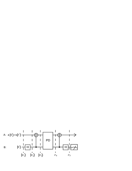
FIG. 2.: Circuit for encoding and decoding. Qubit $A$ is the input qubit. $H$ is the Hadamard transformation, and the symbol next to $H$ is a controlled-not with the dot and circle being the control and target bits. $|\psi_{1-3}\rangle$ are given by Eqs.(25)-(27). $\rho_{4}$, $\rho_{5}$ are mixtures of the states in Eqs.(20)-(23) and in Eqs.(29)-(32). A phase error in either one of the qubits will be revealed by qubit $B$ being in $|1\rangle$ after decoding, and in that case, qubit $A$ will be rejected.

To encode the input qubit, a Hadamard transformation, $H$, is applied to the ancilla, followed by a controlled-not from the ancilla to qubit $A$ (written as $C\!\!N_{ba}$). Let $A$ and $B$ be the first and second label. Then, the two operations have matrix representations

$$H=\frac{1}{\sqrt{2}}\left[\begin{array}[]{cc}{1}&{1}\\ {1}&{-1}\end{array}\right]~{}~{}C\!\!N_{ba}=\left[\begin{array}[]{cccc}{1}&{0}&{0}&{0}\\ {0}&{0}&{0}&{1}\\ {0}&{0}&{1}&{0}\\ {0}&{1}&{0}&{0}\end{array}\right]\,,$$ (24)

and the qubits transform as (Fig. 2)

$$|\psi_{1}\rangle = (a|0\rangle+b|1\rangle)|0\rangle$$ (25)

$$\stackrel{{\scriptstyle I\otimes H}}{{\longrightarrow}}|\psi_{2}\rangle = \frac{1}{\sqrt{2}}(a|0\rangle+b|1\rangle)(|0\rangle+|1\rangle)$$ (26)

$$\stackrel{{\scriptstyle C\!\!N_{ba}}}{{\longrightarrow}}|\psi_{3}\rangle = \frac{1}{\sqrt{2}}(a|0\rangle+b|1\rangle)|0\rangle+(a|1\rangle+b|0\rangle)|1\rangle$$ (27)

$$= \frac{1}{\sqrt{2}}(a(|00\rangle+|11\rangle)+b(|01\rangle+|10\rangle)\,,$$ (28)

where Eq.(28) is the desired encoded state.

The decoding operation is the inverse of the encoding operation (see Fig. 2) so as to recover the input $(a|0\rangle+b|1\rangle)|0\rangle$ in the absence of errors. Phase errors lead to other decoded outputs. The possible decoded states are given by:

$$|\psi_{II}\rangle \stackrel{{\scriptstyle dec}}{{\Rightarrow}} (a|0\rangle+b|1\rangle)|0\rangle$$ (29)

$$|\psi_{ZI}\rangle \Rightarrow (a|0\rangle-b|1\rangle)|1\rangle$$ (30)

$$|\psi_{IZ}\rangle \Rightarrow (a|0\rangle+b|1\rangle)|1\rangle$$ (31)

$$|\psi_{ZZ}\rangle \Rightarrow (a|0\rangle-b|1\rangle)|0\rangle\,.$$ (32)

Note that the ancilla becomes $|1\rangle$ upon decoding if and only if a single phase error has occurred. Moreover, qubits A and B are in product states but they are classically correlated. Therefore, syndrome can be read out by a projective measurement on $B$ without measuring the encoded state. The decoding operation transforms the codeword space and its orthogonal complement to the subspaces spanned by $|0\rangle$ and $|1\rangle$ in qubit $B$, while all the encoded information, either with or without error, goes to qubit $A$.

We illustrate the role of entanglement in the digitization and detection of errors as follows. Suppose the error is a phase shift on qubit $A$: $|0\rangle\rightarrow|0\rangle$, $|1\rangle\rightarrow e^{i\theta}|1\rangle$. Then, the encoded state becomes

$$\frac{1}{\sqrt{2}}\left[\rule{0.0pt}{10.33327pt}a(|00\rangle+e^{i\theta}|11\rangle)+b(e^{i\theta}|10\rangle+|01\rangle)\right]$$ (33)

$$= \frac{1}{\sqrt{2}}\frac{1+e^{i\theta}}{2}\left[\rule{0.0pt}{10.33327pt}a(|00\rangle+|11\rangle)+b(|10\rangle+|01\rangle)\right]$$ (34)

$$+ \frac{1}{\sqrt{2}}\frac{1-e^{i\theta}}{2}\left[\rule{0.0pt}{10.33327pt}a(|00\rangle-|11\rangle)+b(-|10\rangle+|01\rangle)\right]\,.$$ (35)

The decoded state is now a superposition of the states given by Eqs.(29) and (30):

$$\frac{1}{\sqrt{2}}\frac{1+e^{i\theta}}{2}(a|0\rangle+b|1\rangle)|0\rangle+\frac{1}{\sqrt{2}}\frac{1-e^{i\theta}}{2}(a|0\rangle-b|1\rangle)|1\rangle\,.$$ (36)

Measurement of qubit $B$ projects it to either $|0\rangle$ or $|1\rangle$. Because of entanglement, qubit $A$ is projected to having no phase error, or a complete phase flip.

We quantify the error correcting effect of coding using the discrete interpretation of the noise process, leaving a full discussion of the fidelity to Section III. Recall from Eq.(15) that the errors $I\otimes I$, $I\otimes\sigma_{z}$, $\sigma_{z}\otimes I$, and $\sigma_{z}\otimes\sigma_{z}$ occur with probabilities $(1-p_{a})(1-p_{b})$, $(1-p_{a})p_{b}$, $p_{a}(1-p_{b})$ and $p_{a}p_{b}$ respectively, and only in the first and the last cases will the output state be accepted. The probability of accepting the output state is $(1-p_{a})(1-p_{b})+p_{a}p_{b}$ whereas the probability of accepting the correct state is $(1-p_{a})(1-p_{b})$. The conditional probability of a correct, accepted state is therefore

$$\frac{(1-p_{a})(1-p_{b})}{(1-p_{a})(1-p_{b})+p_{a}p_{b}}\approx 1-p_{a}p_{b}\,$$ (37)

for small $p_{a}$, $p_{b}$. The code improves the conditional error probability to second order, as a result of screening out the first order erroneous states.

We conclude this section with a discussion of some properties of the two bit code. First, the code also applies to mixed input states since the code preserves all constituent pure states in the mixed input. Second, we show here that two qubits are the minimum required to encode one qubit and to detect any phase errors. Let ${\cal C}$ be the 2-dimensional codeword space and $E$ be a non-trivial error to be detected. For phase damping, $E$ is unitary and therefore $E{\cal C}$ is also 2-dimensional. Moreover, ${\cal C}$ and $E{\cal C}$ must be orthogonal if $E$ is to be detected. Therefore the minimum dimension of the system is $4$, which requires two qubits. However, using only two qubits implies other intrinsic limitations. First, the code can detect but cannot distinguish errors. Therefore, it cannot correct errors. Moreover, $|\psi_{IZ}\rangle$ decodes to a correct state in spin $A$ which is rejected. These affect the absolute fidelity (the overall probability of successful recovery) but not the conditional fidelity (the probability of successful recovery if the state is accepted). Second, the error $\sigma_{z}\otimes\sigma_{z}$ cannot be detected. This affects both fidelities but only in second order. To understand why these limitations are intrinsic, let $\{E_{k}\}$ be the set of non-trivial errors to be detected. Since $E_{k}{\cal C}$ has to be orthogonal to ${\cal C}$ for all $k$, and since ${\cal C}$ has a unique orthogonal complement of dimension 2 in a two bit code, it follows that all $E_{k}{\cal C}$ are equal, and it is impossible to distinguish (and correct) the different errors. By the same token, for any distinct errors $E_{k^{\prime}}$ and $E_{k}$, $E_{k^{\prime}}E_{k}{\cal C}={\cal C}$ because they are both orthogonal to $E_{k^{\prime}}{\cal C}$, which has a unique 2-dimensional orthogonal complement. Therefore, a two bit code that detects single phase errors can never detect double errors. Finally, since a detection code cannot correct errors, it can only improve the conditional fidelity of the accepted states but not the absolute fidelity. Here, we only remark that the conditional fidelity is a better measure in our experiments due to the bulk system used to implement the two bit code. A discussion of fidelity measures in our experiments and quantum error correction in bulk systems will be postponed until Sections III and VI. The system in which the two bit code is implemented will be described next.

C Bulk NMR Quantum Computation

Nuclear spin systems are good candidates for quantum computers for many reasons. Nuclear spins can have long coherence times. Coupled operations involving multiple qubits are built in as coupling of spins within molecules. Complex sequences of operations can be programmed and carried out easily using modern spectrometers. However, the signal from a single spin is so weak that detection is not feasible with current technology unless a bulk sample of identical spin systems is measured. These identical systems run the same quantum computation in classical parallelism. Computation can be performed at room temperature starting with mixed initial states by distilling the signal of the small excess population in the desired ground state. How NMR quantum computation can be done is described in detail in the following.

The quantum system (hardware)   In our two bit NMR system, $|0\rangle$ and $|1\rangle$ describe the ground and excited states of the nuclear spin (the states aligned with and against an externally applied static magnetic field ${\bf B}_{0}$ in the $+\hat{z}$ direction). As in the previous section, we call the spins denoted by the first and second registers $A$ and $B$. The reduced Hamiltonian for our system is well approximated by ($\hbar=1$) [27, 28] (see also Fig. 3)

$${\cal H}=-\frac{\omega_{a}}{2}{\sigma}_{z}\otimes I-\frac{\omega_{b}}{2}I\otimes{\sigma}_{z}+\frac{\pi J}{2}{\sigma}_{z}\otimes{\sigma}_{z}+{\cal H}_{env}\,.$$ (38)

The first two terms on the right hand side of Eq.(38) are Zeeman splitting terms describing the free precession of spins $A$ and $B$ about the $-\hat{z}$ direction with frequencies $\omega_{a}/2\pi$ and $\omega_{b}/2\pi$. The third term describes a spin-spin coupling of $J$ Hz which is electron mediated. It is known as the $J$ coupling. ${\cal H}_{env}$ represents coupling to the reservoir, such as interactions with other nuclei, and higher order terms in the spin-spin coupling.

Universal set of quantum logic gates   A set of logic gates is universal if any operation can be approximated by some suitable sequence of gates chosen from the set. Depending on whether computation is fault-tolerant or not, the minimun requirements for universality are different. In the latter case, any coupled two-qubit operation together with the set of all single qubit transformations form a universal set of quantum gates [29, 30, 31, 32]. Both requirements are satisfied in NMR as follows.

Single qubit rotations   Spin flip transitions between the two energy eigenstates can be induced by pulsed radio frequency (RF) magnetic fields. These fields, oriented in the $\hat{x}\hat{y}$-plane perpendicular to ${\bf B}_{0}$, selectively address either $A$ or $B$ by oscillating at angular frequencies $\omega_{a}$ or $\omega_{b}$. In the classical picture, an RF pulse along the axis $\hat{\eta}$ rotates a spin about $\hat{\eta}$ by an angle $\theta$ proportional to the product of the pulse duration and amplitude of the oscillating magnetic field. In the quantum picture, the rotation operator $e^{-i\frac{\theta}{2}\vec{\sigma}\cdot\hat{\eta}}$ rotates the Bloch vector (Eq.(8)) likewise. Throughout the paper, we denote rotations of $\pi/2$ along the $\hat{x}$ and $\hat{y}$ axes for spins $A$ and $B$ by $X_{a}$, $Y_{a}$, $X_{b}$, and $Y_{b}$ with respective matrix representations $e^{-i\frac{\pi}{4}\sigma_{x}\otimes I}$, $e^{-i\frac{\pi}{4}\sigma_{y}\otimes I}$, $e^{-i\frac{\pi}{4}I\otimes\sigma_{x}}$, and $e^{-i\frac{\pi}{4}I\otimes\sigma_{y}}$. The rotations in the reverse directions are denoted by an additional “bar” above the symbols of the original rotations, such as $\overline{X}_{a}$. The angle of rotation is given explicitly when it differs from $\pi/2$. This set of rotations generates the Lie group of all single qubit operations, $SU(2)$. For example, the Hadamard transformation can be written as $H=ie^{-i\frac{3\pi}{4}\sigma_{y}}e^{i\frac{\pi}{2}\sigma_{x}}$ which can be implemented in two pulses.

Coupled operations   Quantum entanglement, essential to quantum information processing, can be naturally created by the time evolution of the system. In the respective rotating frames of the spins (tracing the free precession of the uncoupled spins), only the $J$-coupling term, $e^{-i\frac{\pi Jt}{2}\sigma_{z}\otimes\sigma_{z}}$, is relevant in the time evolution. Entanglement is created because the evolution depends on the state of both spins. A frequently used coupled “operation” is a time delay of $\frac{1}{2J}$, denoted by $\tau$, which corresponds to the evolution $e^{-i\frac{\pi}{4}\sigma_{z}\otimes\sigma_{z}}$. For instance, appending $\tau$ with the single qubit rotations $e^{i\frac{\pi}{4}\sigma_{z}\otimes I}$ and $e^{i\frac{\pi}{4}I\otimes\sigma_{z}}$ about the $-\hat{z}$ axes of $A$ and $B$, we implement the unitary operation

$$\chi=e^{i\pi/4}\left[\begin{array}[]{cccc}{1}&{0}&{0}&{0}\\ {0}&{1}&{0}&{0}\\ {0}&{0}&{1}&{0}\\ {0}&{0}&{0}&{-1}\end{array}\right]\,,$$ (39)

which is a cross-phase modulation between the two qubits. Together with the set of all single qubit transformations, $\chi$ completes the requirement for universality. For instance, the controlled-not, $C\!\!N_{ba}$, mentioned in the previous section, can be written as $(H\otimes I)~{}\chi~{}(H\otimes I)$, and can be implemented by concatenating the sequences for each constituent operation. It is also crucial that the free evolution which leads to creation of entanglement can be reversed by applying refocusing $\pi$-pulses, such that creation of entanglement between qubits can be stopped. This technique will be described in detail later.

Measurement   The measured quantity in NMR experiments is the time varying voltage induced in a pick-up coil in the $\hat{x}\hat{y}$-plane:

$$V(t)=-V_{0}Tr\left[\rule{0.0pt}{9.04166pt}\right. e^{-i{\cal H}t}\rho(0)e^{i{\cal H}t}$$ (40)

$$\times(\hskip 2.15277pt(i\sigma_{x}+\sigma_{y}) \otimes I+I\otimes(i\sigma_{x}+\sigma_{y})\hskip 2.15277pt)\left.\rule{0.0pt}{9.04166pt}\right].$$ (41)

The signal $V(t)$, known as the free induction decay (FID), is recorded with a phase-sensitive detector. In Eq.(41), the onset of acquisition of the FID is taken to be $t=0$. If the density matrix $\rho(0)$ has Pauli matrix decomposition $\rho(0)=\sum_{i,j=0}^{3}c_{ij}\sigma_{i}\otimes\sigma_{j}$ where $\sigma_{0,1,2,3}$ are the identity matrix and $\sigma_{x,y,z}$ respectively, then the spectrum of $V(t)$ has four lines at frequencies $\frac{\omega_{a}}{2\pi}+\frac{J}{2}$, $\frac{\omega_{a}}{2\pi}-\frac{J}{2}$, $\frac{\omega_{b}}{2\pi}+\frac{J}{2}$, $\frac{\omega_{b}}{2\pi}-\frac{J}{2}$, with corresponding integrated areas (“peak integrals”)

$$I_{a_{high}} = -\left[\rule{0.0pt}{10.33327pt}i(c_{10}-c_{13})+c_{20}-c_{23}\right]$$ (42)

$$I_{a_{low}} = -\left[\rule{0.0pt}{10.33327pt}i(c_{10}+c_{13})+c_{20}+c_{23}\right]$$ (43)

$$I_{b_{high}} = -\left[\rule{0.0pt}{10.33327pt}i(c_{01}-c_{31})+c_{02}-c_{32}\right]$$ (44)

$$I_{b_{low}} = -\left[\rule{0.0pt}{10.33327pt}i(c_{01}+c_{31})+c_{02}+c_{32}\right]\,.$$ (45)

Note that the expression $c_{10}-c_{13}$ ($c_{10}+c_{13}$) occuring in the high (low) frequency line of spin $A$ is the coefficient of $\sigma_{x}\otimes|1\rangle\langle 1|~{}(|0\rangle\langle 0|)$ in $\rho(0)$. Similarly, $c_{20}-c_{23}$ ($c_{20}+c_{23}$) is the coefficient of $\sigma_{y}\otimes|1\rangle\langle 1|~{}(|0\rangle\langle 0|)$. They signify transitions between the states $|0\rangle\leftrightarrow|1\rangle$ for spin $A$ when spin $B$ is in $|1\rangle$ ($|0\rangle$). Similar observations hold for the high and low lines of spin $B$.

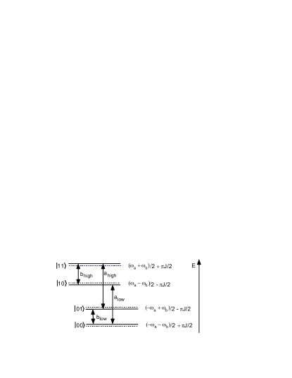
FIG. 3.: Energy diagram for the two-spin nuclear system. The transitions labelled $a_{low}$, $a_{high}$, $b_{low}$ and $b_{high}$ refer to transitions $(|0\rangle\leftrightarrow|1\rangle)|0\rangle$, $(|0\rangle\leftrightarrow|1\rangle)|1\rangle$, $|0\rangle(|0\rangle\leftrightarrow|1\rangle)$ and $|1\rangle(|0\rangle\leftrightarrow|1\rangle)$ respectively.

Thermal States   In bulk NMR quantum computation at room temperature, a pure initial state is not available due to large thermal fluctuations ($\hbar\omega_{a},~{}\hbar\omega_{b}\ll kT$). Instead, a convenient class of initial states arises from the thermal equilibrium states (thermal states). In the energy eigenbasis, the density matrix is diagonal with diagonal entries proportional to the Boltzmann factors, in other words, $\rho_{th}=\frac{1}{{\cal Z}}e^{-\frac{{\cal H}}{kT}}$, where $kT$ is the thermal energy and ${\cal Z}$ is the partition function normalization factor. At room temperature, $\langle\frac{{\cal H}}{kT}\rangle\approx 10^{-6}$, ${\cal Z}\approx\mbox{Dim}(\rho_{th})$ and $\rho_{th}\approx(I-\frac{{\cal H}}{kT})/\mbox{Dim}(\rho_{th})$ to first order. For most of the time, the identity term in the above expansion is omitted in the analysis for two reasons. First, it does not contribute to any signal in Eqs.(42)-(45). Physically, it represents a completely random mixture which is isotropic and, by symmetry, has no net magnetization at any time. Second, the identity is invariant under a wide range of processes. Processes which satisfy ${\cal E}(I)=I$ are called unital. These include all unitary transformations and phase damping. Under unital processes, the evolution of the state is completely determined by the evolution of the deviation from identity [6, 9], in which case the identity can be neglected.

The unitality assumption is a good approximation in our system. The main cause of non-unitality is amplitude damping. In general, for a non-unital but trace preserving process ${\cal E}$, the observable evolution of the deviation can be understood as follows [33]. Rewriting

$$\rho=\upsilon I+\rho_{\delta}$$ (46)

where $\rho_{\delta}=\rho-\upsilon I$ is the traceless deviation from the identity and $\upsilon=1/\mbox{Dim}(\rho)$. Then,

$${\cal E}(\rho) = \upsilon I+\tilde{\rho}_{\delta}$$ (47)

$$\tilde{\rho}_{\delta} = \upsilon({\cal E}(I)-I)+{\cal E}(\rho_{\delta})\,.$$ (48)

The observed evolution of the deviation is $\rho_{\delta}\rightarrow\tilde{\rho}_{\delta}$. The second term in Eq.(48) comes from the evolution of $\rho_{\delta}$ when the identity is neglected, and the first term is the correction due to non-unitality. In our experiment, amplitude damping is slow compared to all other time scales, therefore ${\cal E}(I)-I$ is small and can be treated as a small extra distortion of the state when making the unitality assumption.

Temporal labelling   One convenient method to create arbitrary initial deviations from the thermal mixture is temporal labelling [9, 34]. The idea is to add up the results of a series of experiments that begin with different preparation pulses before the intended experiment, so as to cancel out the signals from the undesired components in the initial thermal mixture. Mathematically, let $\{P_{k}\}$ be the set of initial pulses and ${\cal E}(\rho)$ be the intended computation process. By linearity, $\sum_{k}{\cal E}(P_{k}\rho_{th}P_{k}^{\dagger})={\cal E}(\sum_{k}P_{k}\rho_{th}P_{k}^{\dagger})$. Summing over the experimental results (on the left side) is equivalent to performing the experiment with initial state $\sum_{k}P_{k}\rho_{th}P_{k}^{\dagger}$ (on the right side). Temporal labelling assumes the repeatability of the experiments, which is true up to small fluctuations.

Example   As an example of the above theories, consider applying the pulse sequence in Fig. 4 to the thermal state.

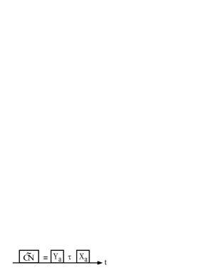
FIG. 4.: Pulse sequence for $\tilde{C\!\!N}$. Time runs from left to right.

The pulses are short compared to other relevant time scales. Therefore, other changes of the system during the pulses are ignored. The unitary operation implemented by the above sequence is given by

$$\tilde{C\!\!N} = e^{-i\frac{\pi}{4}\sigma_{x}\otimes I}e^{-i\frac{\pi}{4}\sigma_{z}\otimes\sigma_{z}}e^{-i\frac{\pi}{4}\sigma_{y}\otimes I}$$ (49)

$$= \frac{1}{\sqrt{2}}\left[\begin{array}[]{cccc}{1-i}&{0}&{0}&{0}\\ {0}&{0}&{0}&{-1-i}\\ {0}&{0}&{1+i}&{0}\\ {0}&{1-i}&{0}&{0\par}\end{array}\right]\,,$$ (54)

similar to $C\!\!N_{ba}$ described in Section II C.

The deviation density matrix of the thermal state is proportional to $-{\cal H}$. Neglecting the $J$-coupling term, which is much smaller than the Zeeman terms,

$$\rho_{th}\sim\frac{\omega_{a}}{2}~{}\sigma_{z}\otimes I+\frac{\omega_{b}}{2}~{}I\otimes\sigma_{z}$$ (55)

$$= \frac{1}{2}\mbox{ Diag}(\omega_{a}+\omega_{b},\omega_{a}-\omega_{b},-\omega_{a}+\omega_{b},-\omega_{a}-\omega_{b})\,$$ (56)

where “Diag” indicates a diagonal matrix with the given elements. For simplicity, we omit the proportionality constant in Eq.(55), and rename the right hand side as $\rho_{th}$. The sequence transforms $\rho_{th}$ to

$$\rho_{cn}=\tilde{C\!\!N}\rho_{th}\tilde{C\!\!N}^{\dagger}$$ (57)

$$= \frac{1}{2}\mbox{ Diag}(\omega_{a}+\omega_{b},-\omega_{a}-\omega_{b},-\omega_{a}+\omega_{b},\omega_{a}-\omega_{b})$$ (58)

$$= \frac{\omega_{a}}{2}~{}\sigma_{z}\otimes\sigma_{z}+\frac{\omega_{b}}{2}~{}I\otimes\sigma_{z}\,,$$ (59)

in which the populations of $|01\rangle$ and $|11\rangle$ are interchanged. Therefore, $\tilde{C\!\!N}$ and $C\!\!N_{ba}$ act in the same way on the thermal state.

By inspection of Eqs.(55) and (59), it can be seen that $\rho_{th}$ and $\rho_{cn}$ have zero peak integrals given by Eqs.(42)-(45). To obtain more information about the states, a readout pulse $X_{a}$ can be applied to transform the two states to

$$\rho_{th}^{\prime}=-\frac{\omega_{a}}{2}~{}\sigma_{y}\otimes I+\frac{\omega_{b}}{2}~{}I\otimes\sigma_{z}$$ (60)

and

$$\rho_{cn}^{\prime}=-\frac{\omega_{a}}{2}~{}\sigma_{y}\otimes\sigma_{z}+\frac{\omega_{b}}{2}~{}I\otimes\sigma_{z}\,.$$ (61)

Now, in $\rho_{th}^{\prime}$ is a term $\sigma_{y}\otimes I$ with coefficient $c_{20}=-\frac{\omega_{a}}{2}$ which contributes to two spectral lines at $\frac{\omega_{a}}{2\pi}\pm\frac{J}{2}$ with equal and positive, real peak integrals. The readout pulse transforms the unobservable coefficient $c_{30}$ in $\rho_{th}$ to the observable $-c_{20}$ in $\rho_{th}^{\prime}$, yielding information on the state before the readout pulse. Similarly, $\rho_{cn}^{\prime}$ has a $\sigma_{y}\otimes\sigma_{z}$ term with coefficient $c_{23}=-\frac{\omega_{a}}{2}$ which gives rise to two spectral lines with real and opposite peak integrals (Fig. 5). All outputs in our experiments are peak integrals of this type carrying information on the decoded states.

FIG. 5.: (a) Spectrum of $A$ after a readout pulse on the thermal state. (b) Spectrum of $A$ after $\tilde{C\!\!N}$ and a readout pulse.

III Two bit code in NMR

We now describe how the two bit code experiment can be implemented in an ensemble of two-spin systems. Modifications of the standard theories in Section II B are needed. These include methods for state preparation, designing encoding and decoding pulse sequences, methods to store the qubit with controllable phase damping, and finally methods to read out the decoded qubit. Fidelity measures for deviation density matrices are also defined.

Spins $A$ and $B$ are designated to be the input and the ancilla qubits respectively. The output states of spin $A$ are reconstructed from the peak integrals at frequencies $\omega_{a}/2\pi\pm J/2$. Fig. 6 schematically summarizes the major steps in the experiments, with details given in the text.

Some notation is defined as follows. Initial states and input states refer to $\rho_{0}$ and $\rho_{1}$ in Fig. 6. The phrase “ideal case” refers to the scenario of having perfect logical operations throughout the experiments and pure phase damping during storage.

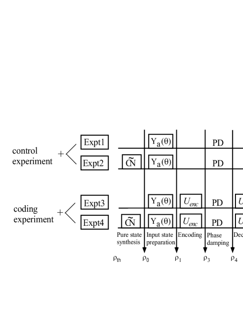
FIG. 6.: Schematic diagram for the two-bit code experiment. $\tilde{C\!\!N}$ is used to prepare the initial state. $Y_{a}(\theta)$ is a variable angle rotation applied to prepare an arbitrary input state, which is then subject to phase damping (PD). In the coding experiment, encoding and decoding operations, $U_{enc}$ and $U_{dec}$, are performed before and after phase damping, whereas in the control experiment, these operations are omitted. $X_{a}$ is used as a readout pulse on $A$ to determine the output state $\rho_{5}$ in spin $A$. $\rho_{i}$ corresponds to $|\psi_{i}\rangle$ or $\rho_{i}$ in Fig. 2. Details are described in the text.

Initial state preparation   It is necessary to initialize spin $B$ to $|0\rangle$ before the experiment. This can be done with temporal labeling using two experiments: the first experiment starts with no additional pulses; the second experiment starts with $\tilde{C\!\!N}$ (Fig. 4). Therefore, the equivalent initial state is $\rho_{th}+\rho_{cn}$ (all symbols are as defined in the example in Section II C):

$$\left[\begin{array}[]{cccc}{\omega_{a}+\omega_{b}}&{0}&{0}&{0}\\ {0}&{-\omega_{b}}&{0}&{0}\\ {0}&{0}&{-\omega_{a}+\omega_{b}}&{0}\\ {0}&{0}&{0}&{-\omega_{b}}\end{array}\right]$$ (66)

$$= \omega_{a}~{}\sigma_{z}\otimes|0\rangle\langle 0|+\omega_{b}~{}I\otimes\sigma_{z}\,.$$ (67)

The first term in Eq.(67) is the desired initial state. The second term cannot affect the observable of interest, the spectrum at $\omega_{a}/2\pi$, because of the following. The identity in $A$ is invariant under the preparation pulse $Y_{a}(\theta)$. The input state is thus the identity, which has no coherence to start with. Therefore, the output state after phase damping in both the control and the coding experiment is still the identity. This is non-trivial in the coding experiment. However, inspection of Eqs.(29)-(32) shows that spin $A$ is changed at most by a phase in the coding experiment. While Eqs.(29)-(32) applies only to the case when $B$ starts in $|0\rangle$, the result can be generalized to any arbitrary diagonal density matrix in $B$ (proof omitted). It follows from Eqs.(42)-(45) that the second term is not observable in the output spectrum of $A$.

In contrast, the input state in spin $A$ can be a mixed state as given by the first term in Eq.(67), since the phase damping code is still applicable. Different input states can be prepared by rotations about the $\hat{y}$-axis of different angles $\theta\in[0,\pi]$ to span a semi-circle in the Bloch sphere in the $\hat{x}\hat{z}$-plane. Due to axisymmetry of phase damping (Eq.(6)), these states suffice to represent all states to test the code.

We conclude with an alternative interpretation of the initial state preparation. Let the fractional populations of $|00\rangle$, $|01\rangle$, $|10\rangle$ and $|11\rangle$ be $p_{00}$, $p_{01}$, $p_{10}$ and $p_{11}$ in the thermal state. Then, the initial state after temporal labelling is

$$(p_{01}+p_{11})~{}I\otimes|1\rangle\langle 1|+2\hskip 2.15277ptp_{10}~{}I\otimes|0\rangle\langle 0|$$ (68)

$$+~{}2\hskip 2.15277pt(p_{00}-p_{10})~{}|00\rangle\langle 00|\,,$$ (69)

where the identity term is not omitted, unlike Eq.(67). Temporal labelling serves to randomize spin $A$ in the first term in Eq.(69) when $B$ is $|1\rangle$. We have shown previously that the identity input state of $A$ is preserved throughout both the coding and the control experiments in the ideal case. Consequently, only the last term in Eq.(69) contributes to any detectable signals in all the experiments, and we can consider the last term as the initial state.

Having justified both pictures using the first term in Eq.(67) and the last term in Eq.(69) as initial state, both will be used throughout rest of the paper.

Encoding and decoding   The original encoding and decoding operations are composed of the Hadamard transformation and $C\!\!N_{ba}$, as defined in Section II C. The actual sequences can be simplified and are shown in Fig. 7.

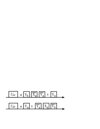
FIG. 7.: Pulse sequences to implement the encoder $U_{enc}$ and the decoder $U_{dec}$. Time runs from left to right. $X(Y)_{a(b)}$ and $\tau$ are as defined in Section II C.

The operator $U_{enc}$ can be found by multiplying the component operators in Fig. 7, giving

$$U_{enc}=\frac{1}{\sqrt{2}}\left[\begin{array}[]{cccc}{1}&{-1}&{0}&{0}\\ {0}&{0}&{i}&{i}\\ {0}&{0}&{1}&{-1}\\ {i}&{i}&{0}&{0\par}\end{array}\right]\,.$$ (70)

The encoded states are slightly different from those in section II B:

$$|0_{L}\rangle = \frac{1}{\sqrt{2}}(|00\rangle+i|11\rangle)$$ (71)

$$|1_{L}\rangle = \frac{1}{\sqrt{2}}(i|01\rangle+|10\rangle)\,,$$ (72)

but the scheme is nonetheless equivalent to the original one.

The decoding operation $U_{dec}$ is given by

$$U_{dec}=\frac{1}{\sqrt{2}}\left[\begin{array}[]{cccc}{1}&{0}&{0}&{-i}\\ {-1}&{0}&{0}&{-i}\\ {0}&{-i}&{1}&{0}\\ {0}&{-i}&{-1}&{0\par}\end{array}\right]=U_{enc}^{\dagger}\,.$$ (73)

The possible decoded outputs are the same as in Section II B except for an overall sign in the single error cases.

Storage   The time delay between encoding and decoding corresponds to storage time of the quantum state. During this delay time, phase damping, amplitude damping and $J$-coupling evolution occur simultaneously. How to make phase damping the dominant process during storage is explained as follows.

First of all, the time constants of amplitude damping, $T_{1}$’s, are much longer than those of phase damping, $T_{2}$’s. Storage times $t_{d}$ are chosen to satisfy $t_{d}\leq T_{2}\ll T_{1}$. This ensures that the effects of amplitude damping are small.

The remaining two processes, phase damping and $J$-coupling, can be considered as independent and commuting processes in between any two pulses since all the phase damping operators commute with the $J$-coupling evolution $\exp(-i\,\sigma_{z}\!\!\otimes\!\sigma_{z}\,\pi\!Jt_{d}/2)$. We choose $Jt_{d}$ to be even integers to approximate the identity evolution. As $J$ is known with limited accuracy, we add refocusing $\pi$-pulses [35] to spin $B$ (about the $\hat{y}$-axis) in the middle and at the end of the phase damping period to ensure trivial evolution under $J$-coupling. These pulses flip the $\hat{z}$ axis for $B$ during the second half of the storage time so that evolution in the first half is always reversed by that in the second half. In this way, controllable amount of phase damping is achieved to good approximation.

Control Experiment   For each storage time $t_{d}$, input state and temporal labelling experiment, a control experiment is performed with the coding and decoding operations omitted. Since phase damping and $J$-coupling can be considered as independent processes, and $J$-coupling is arranged to act trivially, the resulting states illustrate phase damping of spin $A$ without coding.

Output and readout   For an input state prepared with $Y_{a}(\theta)$, the state after encoding, dephasing and decoding ($\rho_{5}$ in Fig. 6) is derived in Appendix A and is given by Eq.(A12) (from here onwards, $\omega_{a}$ is omitted)

$$\rho_{5}^{coded}= \left[\rule{0.0pt}{9.04166pt}\right. \cos\theta~{}(1-p_{a}-p_{b}+2p_{a}p_{b})~{}\sigma_{z}$$ (75)

$$+\sin\theta~{}(1-p_{a}-p_{b})~{}\sigma_{x}\left.\rule{0.0pt}{9.04166pt}\right]~{}\otimes~{}(I+\sigma_{z})/2$$

$$+~{} \left[\rule{0.0pt}{9.04166pt}\right. \cos\theta~{}(p_{a}+p_{b}-2p_{a}p_{b})~{}\sigma_{z}$$ (77)

$$+\sin\theta~{}(-p_{a}+p_{b})~{}\sigma_{x}\left.\rule{0.0pt}{9.04166pt}\right]~{}\otimes~{}(I-\sigma_{z})/2\,.$$

In the control experiment, the corresponding output state is given by (Eq.(A2))

$$\rho_{5}^{control}=\left[\rule{0.0pt}{9.04166pt}\right.\cos\theta~{}\sigma_{z}+(1-2p_{a})\sin\theta~{}\sigma_{x}\left.\rule{0.0pt}{9.04166pt}\right]\otimes(I+\sigma_{z})/2\,.$$ (78)

The initial state used in the derivation of Eq.(78) is the first term in Eq.(67), and the encoding and decoding operations are as given by Eqs.(70) and (73).

In the ideal case, the output state can be read out in a single spectrum. Recall that the coefficients of $-\sigma_{y}\otimes(I\pm\sigma_{z})$ and $-\sigma_{x}\otimes(I\pm\sigma_{z})$ are the real and imaginary parts of the low and the high frequency lines of $A$. Therefore, the coefficients of $-\sigma_{z}\otimes(I\pm\sigma_{z})$ and $-\sigma_{x}\otimes(I\pm\sigma_{z})$ in $\rho_{5}^{coded}$ and $\rho_{5}^{control}$ can be read out as the real and imaginary parts of the low and the high frequency lines of $A$, if $X_{a}$ is applied before acquisition. This pulse transforms the $z$-component of $A$ to the $y$-component leaving the $x$-component unchanged, as described in Section II C. Note that only states with spin $B$ being $|0\rangle$ ($|1\rangle$) contribute to the low (high) frequency line. Therefore, in the coding experiments, the accepted (rejected) states of $A$ can be read out separately in the low (high) frequency line. There are no rejected states in the control experiments.

The rest of the paper makes use of the following notation. “Output states” or “accepted states” refer to the reduced density matrices of $A$ before the readout pulse, and are denoted by $\rho_{a}^{coded}\equiv~{}_{B}\langle 0|\rho_{5}^{coded}|0\rangle_{B}$ and $\rho_{a}^{control}\equiv~{}_{B}\langle 0|\rho_{5}^{control}|0\rangle_{B}$. Rejected states refer to ${}_{B}\langle 1|\rho_{5}^{coded}|1\rangle_{B}$ from the coding experiments.

The accepted and rejected states for a given input as calculated from Eq.(77) and Eq.(78) are summarized in Table I.

$\begin{array}[]{|l|c|c|}\hline\cr{}&{z-\mbox{component}}&{x-\mbox{component}}\\ \hline\cr\hline\cr{\mbox{input state}}&{\cos{\theta}}&{\sin{\theta}}\\ \hline\cr{\mbox{coding expt.:}}&{}\hfil&{}\hfil\\ {\mbox{accepted state}}&{\mbox{(1$-$p${}_{a}$$-$p${}_{b}$+2p${}_{a}$p${}_{b}$) cos$\theta$}}&{\mbox{(1$-$p${}_{a}$$-$p${}_{b}$) sin$\theta$}}\\ {\mbox{rejected state}}&{\mbox{ (p${}_{a}$+p${}_{b}$$-$2p${}_{a}$ p${}_{b}$) cos{$\theta$}}}&{\mbox{ ($-$p${}_{a}$+p${}_{b}$) sin$\theta$}}\\ \hline\cr{\mbox{control expt.:}}&{}\hfil&{}\hfil\\ {\mbox{accepted state}}&{\mbox{ cos$\theta$}}&{\mbox{ (1-2p${}_{a}$) sin$\theta$}}\\ {\mbox{rejected state}}&{\mbox{0}}&{\mbox{0}}\\ \hline\cr\end{array}$

TABLE I.: Input and output states of spin $A$ in the coding and the control experiments.

The output states $\rho_{a}^{coded}$ and $\rho_{a}^{control}$, as predicted by Table I, are plotted in Fig. 8 in the $\hat{x}\hat{z}$-plane of the Bloch sphere of $A$. The north and south poles represent the Bloch vectors $\pm\hat{z}$ ($|0\rangle$ and $|1\rangle$). The time trajectories of various initial states are indicated by the arrows. The Bloch sphere is distorted to an ellipsoid after each storage time. We concentrate on the cross-section in one half of the $\hat{x}\hat{z}$-plane, and call the curve an “ellipse” for convenience. The storage times plotted have equal spacing and correspond to $p_{a}=0,0.071,0.133,0.185,0.230,0.269$. For each ellipse, $p_{b}$ is chosen to be the same as $p_{a}$. The main experimental results will comprise of information of this type.

FIG. 8.: Predicted output states (a) with or (b) without coding. The arrows indicate the direction of time and the ellipses represent snapshots of the original surface of the Bloch sphere.

Fidelity   One can quantify how well the input states are preserved using various fidelity measures. In classical communication, the fidelity can be defined as the probability of successful recovery of the input bit string in the worse case. In quantum information processing, when the input is a pure state, the above definition generalizes to the minimal overlap fidelity,

$${\cal F}=\mbox{min}_{\rho_{in}}\mbox{tr}(\rho_{out}\rho_{in})\,.$$ (79)

We emphasize that Eq.(79) applies to pure input states only. For simplicity, fidelities for mixed input states will not be given here. The reason why Eq.(79) is sufficient for our purpose will become clear later.

When $\rho_{in}$ and $\rho_{out}$ are qubit states of unit trace with respective Bloch vectors $\hat{r}_{in}$ and $\vec{r}_{out}$, Eq.(79) can be rewritten as

$${\cal F}=\mbox{min}_{\hat{r}_{in}}\frac{1}{2}(1+\hat{r}_{in}\cdot\vec{r}_{out})\,.$$ (80)

Recall from Eq.(7) that, for phase damping, when $\hat{r}_{in}=(r_{x},r_{y},r_{z})$, $\vec{r}_{out}=(e^{-\lambda t}r_{x},e^{-\lambda t}r_{y},r_{z})$. Therefore,

$$\hat{r}_{in}\cdot\vec{r}_{out} = e^{-\lambda t}(r_{x}^{2}+r_{y}^{2})+r_{z}^{2}$$ (81)

$$= -2p(r_{x}^{2}+r_{y}^{2})+1\,,$$ (82)

where we have used the fact $|\hat{r}_{in}|^{2}=1$ for pure states and $p=(1-e^{-\lambda t})/2$. The minimum in Eq.(80) is attained for input states on the equatorial plane with $r_{x}^{2}+r_{y}^{2}=1$. Therefore

$${\cal F}=1-p=\frac{1}{2}(1+e^{-\lambda t})\,.$$ (83)

With coding, the accepted state is (see Eqs.(29)-(32))

$$\rho_{a}^{coded}=(1-p_{a})(1-p_{b})\rho_{in}+p_{a}p_{b}\sigma_{z}\rho_{in}\sigma_{z}\,.$$ (84)

If one considers the conditional fidelity in the accepted state, $\rho_{out}$ in Eq.(79) should be taken as the post measurement density matrix,

$$\rho_{out} = \frac{\rho_{a}^{coded}}{\mbox{tr}(\rho_{a}^{coded})}=\frac{\rho_{a}^{coded}}{(1-p_{a})(1-p_{b})+p_{a}p_{b}}$$ (85)

$$\approx (1-p_{a}p_{b})\rho_{in}+p_{a}p_{b}\sigma_{z}\rho_{in}\sigma_{z}\,.$$ (86)

Note that the above expression is identical to the expression for single qubit phase damping but with error probability $p=p_{a}p_{b}$. Therefore, coding changes the conditional error probability to second order, and the conditional fidelity is improved to ${\cal F}_{C}=1-p_{a}p_{b}$.

The amount of distortion can also be summarized by the ellipticities of the “ellipses” that result from phase damping. The ellipticity $\epsilon$ is defined to be the ratio of the major axis to the minor axis. Without coding, the major axis remains unchanged under phase damping, and the minor axis shrinks by a factor of $e^{-\lambda t}$, therefore $\epsilon=e^{\lambda t}$. Using Eq.(83),

$${\cal F}=\frac{1}{2}(1+\frac{1}{\epsilon})\,.$$ (87)

With coding, ${\cal F}_{C}$ is given by the same expression on the right hand side of Eq.(87). In the ideal case, the overlap fidelity and the ellipticity have a one-to-one correspondence. In the presence of imperfections, the overlap fidelity and the ellipticity, one being the minimum of the input-output overlap and the other being an average parameter of distortion, are more effective in reflecting different types of distortion.

We now generalize to new definitions of fidelity for deviation density matrices for the two bit code. In NMR, quantum information is encoded in the small deviation of the state from a completely random mixture. The problem with the usual definitions of fidelity is that they do not change significantly even when the small deviation changes completely. This is true whether the fidelities are defined for pure or mixed input states. To overcome this problem, we introduce the strategy of identifying the initial excess population in $|00\rangle$ as the pure initial state so that usual definitions of fidelity for pure input states are applicable. This improves the sensitivity of the fidelity measures and provides a closer connection to the pure state picture.

The initial state in Eq.(69) can be rewritten as

$$\rho=\alpha\rho^{pure}+(1-\alpha)\rho^{quiet}\,,$$ (88)

where $\alpha=2(p_{00}-p_{10})=\hbar\omega_{a}/2kT$, and

$$\rho^{pure} = |00\rangle\langle 00|$$ (89)

$$\rho^{quiet} \approx \frac{1}{1-\alpha}\left[\rule{0.0pt}{9.04166pt}\right.(p_{01}+p_{11})~{}\mbox{I}\otimes|1\rangle\langle 1|$$ (91)

$$\hskip 43.05542pt+2~{}p_{10}~{}\mbox{I}\otimes|0\rangle\langle 0|\left.\rule{0.0pt}{9.04166pt}\right]\,.$$

It has already been shown that $\rho^{quiet}$ is irrelevant to the evolution and the measurement of $\rho^{pure}$ when all processes are unital. Therefore $\rho^{quiet}$ is neglected and the small signal resulting from the slow non-unital processes will be treated as extra distortion to the observable component. The input state prepared by $Y_{a}(\theta)$ can be written as

$$\rho_{in}=\alpha\rho_{in}^{pure}+(1-\alpha)\rho^{quiet}\,.$$ (92)

For the state change $\rho_{in}\rightarrow{\cal E}(\rho_{in})$, we consider the overlap between $\rho_{in}^{pure}$ and ${\cal E}(\rho_{in}^{pure})$ in place of the overlap between $\rho_{in}$ and ${\cal E}(\rho_{in})$. This defines a new overlap fidelity ${\cal F}_{\delta}=\mbox{min}_{\rho_{in}^{pure}}\mbox{tr}(\rho_{in}^{pure}{\cal E}(\rho_{in}^{pure}))$ $=$ $\mbox{min}_{\hat{r}_{in}}\frac{1}{2}(1+\hat{r}_{in}\cdot\vec{r}_{out})$ similar to the pure state case.

${\cal F}_{\delta}$ can be calculated from the experimental results in the following manner. The measured Bloch vector of $A$, $\vec{r}_{m}$, is proportional to that defined by ${}_{B}\langle 0|{\cal E}(\rho_{in}^{pure})|0\rangle_{B}$. Due to limitations in the measurement process, this proportionality constant $\tilde{\alpha}$ is not known a priori. However, when $\theta=0$ in the control experiment, ${\cal E}(\rho_{in}^{pure})=\rho_{in}^{pure}$ and $\vec{r}_{m}=\tilde{\alpha}\hat{r}_{in}$. Therefore, $\tilde{\alpha}=|\vec{r}_{m}|_{\theta=0}$ can be determined. In other words, $|\vec{r}_{m}|_{\theta=0}$ is used to normalize all other measured output states before using the expression for ${\cal F}_{\delta}$.

The expression for ${\cal F}_{\delta}$ can also be used for the conditional fidelity in the coding experiment if the post-measurement accepted output state is known. This requires $\mbox{tr}(\rho_{a}^{coded})$ $=$ ($1-p_{a}-p_{b}+2p_{a}p_{b}$) to be determined for each storage time. The correct normalization is again given by the output at $\theta=0$, which equals $\vec{r}_{m}=\mbox{tr}(\rho_{a}^{coded})\tilde{\alpha}\hat{r}_{in}$.

In summary, each ellipse obtained in the coding and the control experiment is normalized by the amplitude at $\theta=0$:

$${\cal F}_{\delta}=\mbox{min}_{\hat{r}_{in}}\frac{1}{2}\left[\rule{0.0pt}{10.33327pt}1+\frac{\hat{r}_{in}\cdot\vec{r}_{m}}{|\vec{r}_{m}(\theta=0)|}\right]\,.$$ (93)

It is interesting to note that in contrast to the fidelity measure, the ellipticity measure naturally performs an equivalent normalization, and thus can be used for deviations without modifications.

We now turn to the experimental results, beginning with a description of our apparatus.

IV Apparatus and experimental parameters

We performed our experiments on carbon-13 labeled sodium formate (CHOO^-Na⁺) (Fig. 9) at 15^∘C. The nuclear spins of proton and carbon were used as input and ancilla respectively. Note that the system was heteronuclear. The sodium formate sample was a 0.6 milliliter 1.26 molar solution (8:1 molar ratio with anhydrous calcium chloride) in deuterated water [36]. The sample was degassed and flame sealed in a thin walled, 5mm NMR sample tube.

FIG. 9.: ¹³C-labeled formate. The nuclear spins of the neighboring proton and carbon represent qubits $A$ and $B$.

The time constants of phase damping and amplitude damping are shown in Table II. The fact $T_{1}\ll T_{2}$ ensures that the effect of amplitude damping is small compared to phase damping. The experimental conditions are chosen so that proton and carbon have almost equal $T_{2}$’s: the most theoretically interesting scenario in which identical quantum systems are available for coding. Coding with qubits having very different $T_{2}$’s is described in Appendix B.

The time constants of phase damping and amplitude damping are shown in Table II. The fact $T_{1}\ll T_{2}$ ensures that the effect of amplitude damping is small compared to phase damping. The experimental conditions are chosen so that proton and carbon have almost equal $T_{2}$’s. This eliminates potential bias caused by having a long-lived ancilla when evaluating the effectiveness of coding. This also realizes a common assumption in coding theory that identical quantum systems are available for coding. Subsidiary experiments with qubits having very different $T_{2}$’s are described in Appendix B.

$\begin{array}[]{|c|c|c|}\hline\cr&T_{1}&T_{2}\\ \hline\cr~{}^{1}\mbox{H}{}&~{}~{}9~{}\mbox{s}{}{}&~{}~{}0.65~{}\mbox{s}{}{}\\ ~{}^{13}\mbox{C}{}&~{}~{}13.5~{}\mbox{s}{}{}&~{}~{}0.75~{}\mbox{s}{}{}\\ \hline\cr\end{array}\vspace*{2ex}$

TABLE II.: $T_{1}$’s and $T_{2}$’s for CaCl₂-doped formate at 15^∘C, measured using standard inversion recovery and Carr-Purcell-Meiboom-Gill pulse sequences respectively.

Phase damping arises from constant or low-frequency non-uniformities of the “static” magnetic field which randomize the phase evolution of the spins in the ensemble. Several processes contribute to this inhomogeneity on microscopic or macroscopic scales. Which process dominates phase damping varies from system to system [28]. For instance, intermolecular magnetic dipole-dipole interaction dominates phase damping in a solution of small molecules, whereas the modulation of direct electron-nuclear dipole-dipole interactions becomes more important if paramagnetic impurities are present in the solution. For molecules with quadrupolar nuclei (spin $>$ 1/2), modulation of the quadrupolar coupling dominates phase damping. Other mechanisms such as chemical shift anisotropy can also dominate phase damping in other circumstances. These microscopic field inhomogeneities have no net effects on the static field when averaged over time, but they result in irreversible phase randomization with parameters intrinsic to the sample. Another origin of inhomogeneity comes from the macroscopic applied static magnetic field. In contrast to the intrinsic processes, phase randomization due to this inhomogeneity can be reversed by applying refocusing pulses as long as diffusion of molecules is insignificant.

Phase damping caused by the intrinsic irreversible processes alone has a time constant denoted by $T_{2}$, while the combined process has a shorter time constant denoted by $T_{2}^{*}$. $T_{2}$ is measured by the Carr-Purcell-Meiboom-Gill [35] experiment using multiple refocusing pulses. $T_{2}^{*}$ can be estimated from the line-width of the NMR spectral lines: during acquisition, the signal decays exponentially due to phase damping, resulting in Lorentzian spectral lines with line-width $1/\pi T_{2}^{*}$.

In our experiment, $T_{2}^{*}$’s for proton and carbon were estimated to within 0.05 s to be $\approx$ 0.35 and 0.50 s. The storage times $t_{d}$ were approximately 0, 62, 123, 185, 246, 308 ms ($n/J$ for $n=0,12,24,36,48,60$). The maximum storage time was 120 $\tau$, long compared to the clock cycle and was comparable to $T_{2}^{*}$. The decay constant $\lambda$, defined in Section II A, was given by $\lambda=1/T_{2}^{*}$. The error probabilities after a storage time of $t_{d}$ were $p_{i}=(1-\exp(-t_{d}/T_{2i}^{*}))/2$ for spins $i=A,B$. To reconstruct the ellipse for each storage time, 11 experiments were run with input states spanning a semi-circle in the $\hat{x}\hat{z}$-plane. Each input state was prepared by a $Y_{a}(\theta)$ pulse with $\theta=n\pi/10$ for $n=0,1,\cdots,10$.

All experiments were performed on an Oxford Instruments superconducting magnet of 11.7 Tesla, giving precession frequencies of $\omega_{A}/2\pi$ $\approx$ 500 MHz for proton and $\omega_{B}/2\pi$ $\approx$ 125 MHz for carbon. A Varian ^UNITYInova spectrometer with a triple-resonance probe was used to send the pulsed RF fields to the sample and to measure the FID’s. The RF pulses selectively rotated a particular spin by oscillating on resonance with it. The $\pi$/2 pulse durations were calibrated, and they were typically 8 to 14 $\mu$s. To perform logical operations in the respective rotating frames of the spins, reference oscillators were used to keep track of the free precession of both spins, leaving only the $J$-coupling term of 195.0 Hz in the time evolution. Each FID was recorded for $\approx$ 6.8 s (until the signal had faded completely). The thermal state was obtained after a relaxation time of 80 s ($\gg T_{1}$’s) before each pulse sequence.

Using the above apparatus and procedures, we performed the experiments as outlined in Section III. The experimental results are described in the next section. Tomography results following the evolution of the state are presented in Appendix C.

V Results and discussion

A Decoded Bloch spheres

The output states, $\rho_{a}^{coded}$ and $\rho_{a}^{control}$, obtained as described in Sections III and IV, and the analysis that confirms the correction effects of coding, are presented in this section.

Fig. 10 shows the accepted states in the $\hat{x}\hat{z}$-plane of the Bloch sphere of $A$. $\rho_{5}^{coded}$ and $\rho_{5}^{control}$ are plotted in Figs. 10 a and b. The ellipse for each storage time is obtained by a least-squares fit described later.

FIG. 10.: (a) Experimental data (circles) showing the output states from the coding experiment. Each ellipse (solid line) corresponds to one storage time and is obtained by a least-squares fit (Eq.(100)) to the data. The storage times are $n\times 61.5$ms for $n=0,1,\cdots,5$, and smaller ellipses correspond to increasing $n$. (b) Experimental data (crosses) and fitted ellipses (solid lines) for the control experiment. A replica of figure (a) is plotted in dotted lines for comparison. In both figures, uncertainties in the data are much smaller than the circles and crosses.

The most important feature in Fig. 10 is the reduction of the ellipticities of the ellipses due to coding, which represents partial removal of the distortion caused by phase damping - the signature of error correction. Coding is effective throughout the range of storage times tested.

We quantify the correction effects due to coding using the ellipticities. When deviations from the ideal case such as offsets of the angular positions of the points along the ellipses and attenuation of signal strength with increasing $\theta$ exist, the minimum overlap fidelities and the ellipticities are no longer related by Eq.(87). Since the ellipticity is an average measure of distortion which is less susceptible to scattering of individual data points, we first study the ellipticities. Moreover, since the deviations from the ideal case are small, we can still infer the fidelities from the ellipticities using Eq.(87). A discussion of the discrepancies and the exact overlap fidelities will given later.

Ellipticities   In the ideal case, the ellipticity for each ellipse can be obtained experimentally as

$$\epsilon=\sqrt{\frac{I(\theta=0)}{I(\theta=\frac{\pi}{2})}}\,,$$ (94)

where $I$ denotes the intensity (amplitude square) of the peak integral. $I$ is given by the $\hat{x}$ and $\hat{z}$-components of the output states as

$$I=r_{x}^{2}+r_{z}^{2}\,.$$ (95)

In the ideal case, $I(\theta)$ can be found from Table I:

$$I_{control}(\theta) = 1-4(p_{a}-p_{a}^{2})\sin^{2}\theta$$ (96)

$$I_{coded}(\theta) = (1-p_{a}-p_{b}+2p_{a}p_{b})^{2}$$ (98)

$$-4p_{a}p_{b}(1-p_{a}-p_{b}+p_{a}p_{b})\sin^{2}\theta\,,$$

and both are of the functional form

$$I_{ideal}(\theta) = A+B\sin^{2}\theta\,.$$ (99)

Experimentally, the output Bloch vectors do not form perfect ellipses. We modify Eq.(99) to include signal strength attenuation with increasing $\theta$ and constant offsets in the angular positions:

$$I_{exp}(\theta) = (A+B\sin^{2}(\theta+D))(1-C(\theta+D))\,,$$ (100)

and perform non-linear least-squares fits of the experimental data to determine $A,B,C$ and $D$. The fitted ellipses plotted in Fig. 10 follow from Eq.(100) and the fitted parameters. The ellipticities $\epsilon$ are found using Eq.(94) by interpolating the intensities at $\theta=0$ and $\theta=\frac{\pi}{2}$. The ellipticities are plotted in Fig. 11 a. The uncertainties of the fitted parameters originate from the uncertainties in the data, which are estimated to be $\approx$ 1% for the amplitude and 1.5 degrees for the phase in the measured peak integrals. These uncertainties are propagated numerically to the ellipticities as plotted in Fig. 11 a. Ideal case predictions and simulation results are also plotted in Fig. 11 a. The simulation takes into account the major imperfection in the pulses and will be described later.

FIG. 11.: (a) Ellipticity and (b) inferred fidelity as a function of the storage time in the coding and the control experiments. Error bars represent 95% confidence level.

Error correction   The effectiveness of coding to correct errors is evident when comparing the ellipticities from the coding and the control experiments (Fig. 11 a). Without coding, the ellipticity grows exponentially as $e^{t_{d}/T_{2a}^{*}}$ (for $T_{2a}^{*}$ fitted to be $\approx 0.4s$). With coding, the growth is slowed down, with almost zero growth for small $t_{d}$. The suppression of linear growth of the ellipticity can be further quantified by weighted quadratic fits $\epsilon=c_{0}+c_{1}t_{d}+c_{2}t_{d}^{2}$ to the ellipticities. For the control experiments, $c_{0}=1.00\pm 0.01$, $c_{1}=1.31\pm 0.21$ and $c_{3}=8.8\pm 0.8$ whereas for the the coding experiments, $c_{0}=1.10\pm 0.02$, $c_{1}=-0.24\pm 0.29$ and $c_{3}=3.8\pm 0.9$ ($t_{d}$ in seconds). Therefore, the linear term “vanishes” due to coding. The small negative coefficient for the linear term originates from the scattering of the data point at zero storage time.

To quantify the “cost of the noisy gates” caused by the imperfect pulses, we compare the ellipticities from the coding experiments and from the ideal case, the quadratic fits of which are respectively $\epsilon^{coded}_{expt}=1.10-0.24t_{d}+3.80t_{d}^{2}$ and $\epsilon^{coded}_{ideal}=1.00+0.15t_{d}+2.50t_{d}^{2}$. The imperfections cause the ellipticity to increase by 0.1 at $t_{d}=0$ and this extra distortion decreases with $t_{d}$. We take advantage of the fact that the simulation results are close to the data points but are not as scattered to have a better estimate of this “cost of the noisy gates”. The simulation data can be fitted by $\epsilon^{coded}_{sim}=1.06+0.32t_{d}+2.47t_{d}^{2}$. Compared to the ideal case, the coding operations increase the ellipticity by $\approx$ 0.06 at $t_{d}=0$, and this extra distortion remains almost constant for all $t_{d}$.

The error probabilities as inferred from the ellipticities $p_{\epsilon}=1-{\cal F}_{\epsilon}=\frac{1}{2}(1-\frac{1}{\epsilon})$ are plotted in Fig. 11 b as a function of storage time.

Error correction is also manifested by expressing $p_{\epsilon}$ in the coding experiment as a function of the original $p_{\epsilon}$ in the control experiment, as plotted in Fig. 12. The quadratic fit to the experimental results gives $p^{coded}_{exp}=c_{0}+c_{1}p+c_{2}p^{2}$ where $p$ stands for $p_{\epsilon}$ in the control experiment, $c_{0}=0.047\pm 0.008$, $c_{1}=-0.05\pm 0.12$ and $c_{2}=1.38\pm 0.40$. Therefore, the expected improvement $p\rightarrow p_{a}p_{b}$ is confirmed. Experimentally, the error probabilities are larger than in the ideal case by at most 4.7% and these extra errors decrease with $p$. The quadratic fit to the simulation results (which is a good approximation of the experimental data) gives $p^{coded}_{sim}=0.032-0.032p+1.783p^{2}$ and differs from the ideal case by a constant amount of $\approx 0.033\pm 0.003$ for all $p$, which represents the cost of the noisy gates. In conclusion, coding with noisy gates is still effective in our experiments, even though the noisy gates add a constant amount of distortion.

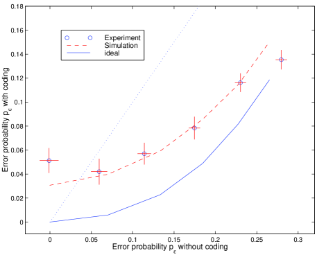
FIG. 12.: Error probabilities in the coding experiments vs the corresponding values in the control experiments. Error bars represent 95% confidence level. The 45^∘ line is plotted as a dotted line.

B Discrepancies

While the data exhibit a clear correction effect, there are notable deviations from the ideal case. First, the ellipses with coding are smaller than their counterparts without coding. This is most obvious when the storage time is zero, in which case the coding and the control experiments should produce equal outputs. Second, the signal strength is attenuated with increasing $\theta$ relative to ideal ellipses. Third, although the data points are well fitted by ellipses, their angular positions are not exactly as expected (“$\theta$-offsets”). Finally, the spacings between the ellipses deviate from expectation. The causes of these discrepancies and their implications on error correction are discussed next.

Gate imperfections: RF field inhomogeneity   The major cause of experimental errors is RF field inhomogeneity, which causes gate imperfections. This was determined by a series of experiments (details of which are not given here), and a thorough numerical simulation, as described below. The physical origin of the problem is as follows. The coil windings produce inhomogeneous RF fields that randomize the angles of rotation among molecules. For a single rotation, the signal averaged over the ensemble decreases exponentially with the pulse duration to good approximation. A measure of the RF field inhomogeneity is the signal strength after a $\pi/2$ pulse. They are measured to be $\approx$ 0.96 and 0.92 for proton and carbon respectively. In other words, a single $\pi/2$ pulse has an error of $\approx$ 4-8%.

RF field inhomogeneity affects our experiments in many ways. First, it attenuates the signal in both the coding and the control experiments, but the effects are much more severe in the coding experiments which have eight extra pulses. For instance, when the storage time is zero, the two experiments should have identical outputs, but the ellipse in the coding experiment is actually 5-15 % smaller. Second, for each ellipse, attenuation increases with $\theta$ as the preparation pulse $Y_{a}(\theta)$ becomes longer.

The effects of the RF field inhomogeneity are complicated, because the errors from different RF pulses are correlated, and the correlation depends on the temporal separation between the pulses and the diffusion rate of the molecules. The correlation time of the RF field inhomogeneity is comparable to the experimental time scales. For this reason, predictions of the effects of RF field inhomogeneity are analytically intractable.

Numerical simulations were performed to model the dominant effects of RF field inhomogeneity. We followed the evolution of the states assuming random RF field strengths drawn from Lorentzian distributions (also known as Cauchy distributions) with means and standard deviations matching pulse calibration and attenuation for the $\pi/2$ pulses. All parameters in the simulation, including $T_{2}^{*}$’s, were determined experimentally without introducing any free parameters. As the exact time correlation function for the errors was unknown, except for numerical evidence of a long correlation time, we assumed perfect correlation in the errors. The simulated ensemble output signal was obtained by Gaussian integration with numerical errors bounded to below 1.5%. The results were shown in Fig. 13.

FIG. 13.: Simulated output states, plotted similarly as in Fig. 10. The simulation results are fitted by ellipses similar to those of the experimental data.

Besides phase damping and error correction effects in the data, the simulations also reproduce extra signal attenuation in the coding experiments. The ellipticities obtained from simulations (see Fig. 11) approximate the experimental values very well. Such agreement to experimental results is surprising in the absence of free parameters in the model. Simulation results allow the discrepancy between the observed and the ideal ellipticities to be explained in terms of the RF field inhomogeneity and allow the “cost of coding” to be better estimated to be the constant 6 % increase in ellipticity or the $\approx$ 3 % increase in error probabilities.

The simulation results also predict increasing attenuation with $\theta$. From the fitted parameter $C$ (see Eq.(100)), the amplitudes at $\theta=\pi$ are $\approx$ 4% weaker than the corresponding values at $\theta=0$ in the simulations. Experimentally, this attenuation increases from $\approx$ 8 to 15% (as storage time increases from 0 to 308 ms) in the control experiments, and remains $\approx$ 8% in the coding experiments. Therefore, RF field inhomogeneity contributes to the attenuation but only partially.

We conclude that RF field inhomogeneity as we have modeled explains the diminished signal strength in the coding experiments. The simulation quantifies the “cost of the noisy gates”. RF field inhomogeneity also explains part of the attenuation with increasing $\theta$. We can also conclude that other discrepancies not predicted by the simulations are not caused by RF field inhomogeneity and these discrepancies are described next.

Other discrepancies   The simulation results show that RF field inhomogeneity does not explain why the attenuation at large $\theta$ increases with storage time without coding, and it does not explain the $\theta$-offsets along the ellipses and the unexpected spacings between them.

The increased attenuation with storage time at large $\theta$ can be caused by amplitude damping. A precise description [37] of amplitude damping during storage is out of scope of this paper and we consider only the dominant effect predicted by a simple picture. Phenomenologically, the loss of energy to the lattice is described in the NMR literature by

$$z(t)=z(\infty)+(z(0)-z(\infty))~{}e^{-t/T_{1}}\,,$$ (101)

where $z(\infty)=1$ is the thermal equilibrium magnetization. As $z(0)=\pm 1$ at $\theta=0$ and $\pi$, we expect no changes at $\theta=0$, but expect $|z|$ at $\theta=\pi$ to decrease by $0-7$ % for $t_{d}\approx 0-308$ ms and $T_{1}\approx 9$ s for proton. Note that refocusing does not affect spin $A$ in the control experiments [38] but it swaps $|0_{L}\rangle$ and $|1_{L}\rangle$ halfway during storage, symmetrizing the amplitude damping effects in the coding experiments. Therefore, we expect increased attenuation with storage time in the control experiments only. This matches our observations that $I(\theta=\pi)$ decreases from 8 to 16 % in the control experiments, and remains 8% in the coding experiments. Moreover, earlier data taken without refocusing (not presented) have the same trend of increased attenuation with storage time in both the coding and the control experiments. These are all in accord with the hypothesis that amplitude damping is causing the observed effect.

The second unexplained discrepancy is that the output states span more than a semi-ellipse in the coding experiment but slightly less than a semi-ellipse in the control experiment. We are not aware of any quantum processes that can be a cause of it. It is notable that the output states and the fitted ellipticities can be used to infer the initial values of $\theta$, and they are roughly proportional to the expected values for each ellipse. The proportionality constants are 5-8 % higher than unity in the coding experiment, and 0-1.6% lower in the control experiments. Moreover, similar effects are observed in many other experimental runs. Therefore, this is likely to be a systematic error.

We have no convincing explanation for the anomalous spacings between the ellipses in the experiment. However, from the fact that all the data points belonging to the same ellipse are well fitted by it, the anomalous spacings are unlikely to be caused by random fluctuations on the time scales of each ellipse-experiment. The effect of the anomalous spacings is reflected in the scattering of the ellipticities of the data, and the large uncertainties in the quadratic fits.

While it is impossible to eliminate or to fully explain these imperfections, it is possible to show that the deviations cannot affect the conclusion that error correction is effective.

Effects of the discrepancies   We now consider the effects of the discrepancies on the ellipticities and the inferred fidelities in the experiments. First of all, radial attenuation of the signal due to RF field inhomogeneity does not affect the ellipticities nor the inferred fidelities (taken as conditional fidelities). Second, different expressions for the “ellipticity” are not equivalent when the output states do not form perfect ellipses. However, they differ by no more than 7 and 3 % in the control and the coding experiments. $\theta$-offsets along the ellipses are not reflected in the ellipticities, resulting in overestimated inferred fidelities. This is bounded by 3%. The scattering of the ellipticities due to anomalous spacings between the ellipses is averaged out with curve-fits to the data. The most crucial point is, none of these effects have a dependence on the storage time that can be mistaken as error correction. Therefore, the effects of error correction can still be confirmed in the presence of all these small discrepancies.

C Overlap fidelity

The two previous subsections dealing with the ellipticities provide an analysis of the global performance of the code. A stricter analysis is provided in this section using the overlap fidelities given by Eq.(93) in Section III. The minimal overlap reflects all defects and deviations hidden in the ellipticities as well as other distortions such as that caused by amplitude damping.

All measurements are normalized using the amplitudes at $\theta=0$ as described in Section III. In the control experiments, the output states at $\theta=0$ are least affected by amplitude damping and RF field inhomogeneity. Therefore, the normalization can be done accurately. In the coding experiment, the signal attenuation at $\theta=0$ due to RF field inhomogeneity can lead to overestimated fidelities. We determine the uncertainties due to RF field inhomogeneity by the following method. For each storage time, the amplitudes of the accepted and the rejected states at $\theta=0$ are summed. The sum is compared with the corresponding amplitude at $\theta=0$ in the control experiment to estimate the attenuation due to RF field inhomogeneity. The effects on the overlap fidelities are bounded to below 2%. The errors in the measured peak integrals are propagated to the fidelities which result in standard deviations no more than 0.7%. We apply similar procedures to the simulation results. The net error probabilities, given by $1-{\cal F}$ for the control and $1-{\cal F}_{C}$ for the coding experiments, are plotted in Fig. 14.

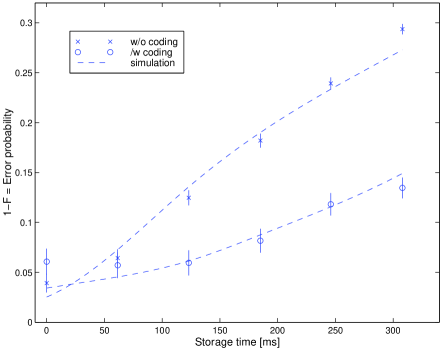
FIG. 14.: Overlap fidelity as defined in Eq.(93). Points indicate experimental data and dashed lines indicate simulation results. Error bars represent 95% confidence level.

The large difference in the rates of growth of error probabilities confirms the effectiveness of coding even when a stricter measure of fidelity is used.

VI Conclusion

We have demonstrated experimentally, in a bulk NMR system, that using a two bit phase damping detection code, the distortion of the accepted output states can be largely removed. These experimental results also provided quantitative measures of the major imperfections in the system. The principle source of errors, RF field inhomogeneity, was studied and a numerical simulation was developed to model our data. Despite the imperfections, a net amount of error correction was observed, when comparing cases with and without coding, and including gate errors in both cases.

Our analysis also addresses several theoretical questions in quantum error correction in bulk samples such as the fidelity measures of deviation density matrices. In the following, we conclude with some observations regarding quantum error correction in bulk systems, including syndrome measurements, the equivalence between error correction and logical labelling [6, 9], the applicability and advantages of detection codes and some issues in signal strength.

Projective syndrome measurements traditionally employed in the standard theory of quantum error correction are impossible in ensemble quantum computation. Measurements via the acquisition of the FID do not reduce individual quantum states and provide only “average syndromes”. Moreover, the quantum states are destroyed after acquisition. However, the important point is that syndrome measurement is not necessary in error correction [39, 13].

In each molecule, the syndrome bits carry the error syndrome for that particular molecule after decoding. These bits can either be used in a controlled-operation to correct the error [39], or in the case of a detection code, to “logically label” the correct and erroneous states. Conversely, logical labelling to obtain effective pure states can be considered as error detection: unsuitable initial states are “detected” and are labelled as “bad” to start with. Both processes involve ejecting the entropy of the system to the ancilla bits. Error detection and logical labelling are therefore similar concepts.

The distinction between correction and detection codes is blurred when using bulk systems. The objective of error correction is to achieve reliable data transmission or information processing with high probability of success. When information is encoded in single systems, encoding with an error detection scheme will fail to provide reliable output for two different reasons: accepting an erroneous state or losing the state upon the detection of an error. Therefore, coding schemes capable of distinguishing and correcting errors are necessary to improve the probability of successful data processing. In contrast, in a bulk sample, a large initial redundancy exists upon preparation, and the combined signal of all the accepted cases forms the output. Therefore, rejection of the erroneous cases results in a reduction of the signal strength in the improved accepted cases without necessarily causing a failure. Detection codes thus provide a tradeoff between probability of error-free computation and signal strength.

As suggested by this analysis, and in concert with our experimental results, it thus makes sense to use detection codes instead of correction codes in bulk quantum computing systems under certain circumstances. Fundamentally, it is valuable to be able to interchange resources depending on their relative costs, This is illustrated by the following simple example. Suppose a total pool of $m$ qubits is available for transmission, and one just wants to correct for single phase flip errors of probability $p$. Using a three bit code, one would obtain an aggregate signal strength of $m/3$, with fidelity $1-3p^{2}$, whereas with a two bit code, the accepted signal strength would be $m(1-2p)/2$, with fidelity $1-p^{2}$. Therefore, when $p\leq 1/6$, the two-qubit code performs better in this model due to its higher rate.

Another example relevant to bulk computation arises when the encoding and decoding circuits fail with probability proportional to the number of elementary gates used. Although errors in consecutive gates can be made to cancel sometimes, this basic scenario is substantiated by our experiment, in which imperfect pulses contribute significantly to the net error. Assume now that we have $n$ molecules, which are either two or three qubit systems. Let us compare the performance of the two and three bit codes, based on the strength of the correct output signal. Because the correction code requires at least three times as many operations as the detection code [40], the figures of merit obtained for the two schemes are $n(1-3p_{g})$ and $n(1-2p)(1-p_{g})$ respectively, where $p_{g}$ is the gate failure probability. In this model, the detection code performs better for $p\leq p_{g}/(1-p_{g})$ due to the simplicity of the coding operations.

A third example is the case of current state NMR quantum computation at room temperature, in which the intrinsic signal strength decreases exponentially with the number of qubits[6, 9, 34]. In this model, the initial signal strength of an effective pure state of $m$ qubits is approximately of order $2^{-m}$, and thus, for an ensemble of $n$ molecules, the signal strengths of the outputs from the correction and detection codes are about $n/8$ and $n(1-2p)/4$ respectively. According to this measure of performance, the detection code outperforms the correction code for $p\leq 1/4$ ($p\leq 0.27$ in our experiments).

If signal strength indeed decreases exponentially with $m$, then some interesting generalizations can be made. For arbitrary qubit errors, a $t$-error detection code has distance $d\geq t+1$, while a $t$-error correction code has distance $d\geq 2t+1$ [26]. If one encodes $k$ bits in $l$, the extra number of qubits used, $l-k$, satisfies the singleton bound [23, 42, 43], $l-k\geq 2d-2$. Therefore, the output signal strengths for detection and correction codes would be approximately proportional to $(1-pf(p))/2^{2t}$ and $1/2^{4t}$, where $f(p)$ is a polynomial. The detection code is thus always better asymptotically in this model[41].

This work illustrates how a careful study of dynamics in bulk quantum systems can provide a valuable opportunity to demonstrate and test theories of quantum information and computation. The development of temporal, spatial, logical, and related labeling techniques opens a window allowing information about the dynamics of single quantum systems to be extracted from bulk systems. Furthermore, by systematically developing an experimental toolbox of quantum circuits and quantum error correction and detection codes, experiments which test multiple particle quantum behavior become increasingly accessible. With improvements in the initial polarization in the systems and new labeling algorithms which do not incur exponential signal loss [44], and with better methods to control the major source of error, the RF field inhomogeneity, we believe that further study of bulk quantum systems will complement the study of single quantum systems, provide new insights into the dynamical behavior of open quantum systems, and further the potential for quantum information processing.

VII Acknowledgments

This work was supported by the DARPA Ultrascale Program under contract DAAG55-97-1-0341. D.L. acknowledges support of an IBM Graduate Fellowship. L.V. acknowledges a Yansouni Family Fellowship under the Stanford Graduate Fellowship program. L.V., X.Z. and D.L. are indebted to Prof. James Harris and Prof. Yoshihisa Yamamoto for their patience and support. We thank Thorsten Hesjedal, Lois Durham and Jody Puglisi for experimental assistance, Nabil Amer, Charles Bennett, Hoi Fung Chau, Hoi-Kwong Lo and Shigeki Takeuchi for enjoyable and helpful discussions, and Rolf Landauer for his guiding wisdom.

A Mixed state description of the two bit code

Recall that the initial state after ancilla preparation is given by $\rho_{0}=\sigma_{z}\otimes(I+\sigma_{z})/2$ (see Eq.(67), with $\omega_{a}$ omitted). After $Y_{a}(\theta)$, the new density matrix is given by

$$\rho_{1}=(\cos\theta\sigma_{z}+\sin\theta\sigma_{x})\otimes(I+\sigma_{z})/2\,.$$ (A1)

Without coding, phase damping changes the density matrix to

$$\rho_{5}^{control}=\left[\rule{0.0pt}{10.33327pt}\cos\theta\sigma_{z}+(1-2p_{a})\sin\theta\sigma_{x}\right]\otimes(I+\sigma_{z})/2\,.$$ (A2)

With coding, the encoding, phase damping, and decoding change the density matrix to $\rho_{3}$, $\rho_{4}$, and $\rho_{5}$:

$$\rho_{3}^{coded} = \cos\theta(\sigma_{z}\otimes\sigma_{z}+\sigma_{y}\otimes\sigma_{x})/2$$ (A3)

$$+ \sin\theta(\sigma_{x}\otimes I+I\otimes\sigma_{y})/2$$ (A4)

$$\rho_{4}^{coded} = \cos\theta(\sigma_{z}\otimes\sigma_{z}+(1-2p_{a})(1-2p_{b})\sigma_{y}\otimes\sigma_{x})/2$$ (A5)

$$+ \sin\theta((1-2p_{a})\sigma_{x}\otimes I+(1-2p_{b})I\otimes\sigma_{y})/2$$ (A6)

$$\rho_{5}^{coded} = \cos\theta\sigma_{z}\otimes(I+(1-2p_{a})(1-2p_{b})\sigma_{z})/2$$ (A7)

$$+ \sin\theta\sigma_{x}\otimes((1-2p_{a})I+(1-2p_{b})\sigma_{z})/2$$ (A8)

$$= \cos\theta\sigma_{z}\otimes\left[\rule{0.0pt}{10.33327pt}(1-p_{a}-p_{b}+2p_{a}p_{b})(I+\sigma_{z})+(p_{a}+p_{b}-2p_{a}p_{b})(I-\sigma_{z})\right]/2$$ (A9)

$$+ \sin\theta\sigma_{x}\otimes\left[\rule{0.0pt}{10.33327pt}(1-p_{a}-p_{b})(I+\sigma_{z})+(-p_{a}+p_{b})(I-\sigma_{z})\right]/2$$ (A10)

$$= \left[\rule{0.0pt}{10.33327pt}\cos\theta(1-p_{a}-p_{b}+2p_{a}p_{b})\sigma_{z}+\sin\theta(1-p_{a}-p_{b})\sigma_{x}\right]\otimes(I+\sigma_{z})/2$$ (A11)

$$+ \left[\rule{0.0pt}{10.33327pt}\cos\theta(p_{a}+p_{b}-2p_{a}p_{b})\sigma_{z}+\sin\theta(-p_{a}+p_{b})\sigma_{x}\right]\otimes(I-\sigma_{z})/2\,.$$ (A12)

Alternative understanding of the code

The operation of the code can be further understood using the above mixed state description. Without coding, the input qubit is stored in the terms $\sigma_{z}\otimes I$ and $\sigma_{x}\otimes I$ which decay at different rates and distort the state asymmetrically. With coding, the input qubit is stored in the terms $(\sigma_{z}\otimes\sigma_{z}+\sigma_{y}\otimes\sigma_{x})$ and $(\sigma_{x}\otimes I+I\otimes\sigma_{y})$ which decay at the same overall rate to first order. The resulting decoded state therefore shrinks radially up to first order.

When subject to phase damping, the points on the Bloch sphere move inwards transversely without coding, distorting the shape axisymmetrically (Fig. 15). In contrast, the points move somewhat radially with coding, preserving the spherical shape better.

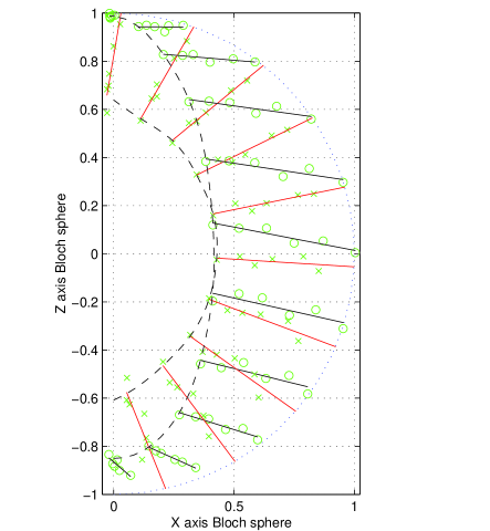
FIG. 15.: Experimental data described in Section V. The solid lines, which are linear fits to the data points, indicate the flow directions of the points on the Bloch sphere subject to phase damping. In the no coding case, the flows are nearly planar, towards the $\hat{z}$-axis, whereas in the encoded case, the flows are nearly radial, towards the center.

B The case of very different T₂’s

While the case of equal $T_{2}$’s is interesting from a theoretical standpoint, different spins in a molecule typically have quite different $T_{2}$’s. To study the two bit code in this regime, we performed experiments with carbon-13 labelled chloroform dissolved in acetone [45, 9]. All parameters were similar to the sodium formate sample, except for the relaxation time constants.

In the chloroform experiment, $T_{1}$’s were 16 s and 18.5 s and $T_{2}$’s were 7.5 s and 0.35 s for proton and carbon respectively. Separate experiments with the ancilla dephasing much slower or faster than the input were performed by interchanging the roles of proton and carbon. $T_{2}^{*}$’s and $t_{d}$’s were as listed in [46]. The ellipticities are shown in Fig. 16.

FIG. 16.: Ellipticities obtained in the chloroform experiments, with (a) proton and (b) carbon as the ancilla. Carbon dephases much faster than proton. Error bars represent 95% confidence level.

From Fig. 16 a, it is apparent that coding almost removes the distortion entirely when a much better ancilla is available. The question is, is coding advantageous over storing in the good ancilla alone? Theoretically, coding is always advantageous because the error probability is always reduced from $p_{i}$ ($i$ being the input spin) to $p_{a}p_{b}$. Fig. 16 b shows that experimentally, such improvement is marginal, because the advantage of coding is offset by the noise introduced. Therefore, when the $T_{2}$’s are very different, the bottle neck is the dephasing of the bad qubit.

C Tomography results at major steps

Quantum state tomography [9] is a procedure to reconstruct the density matrix given a certain set of measurements. In 2-spin NMR systems, eight out of the fifteen coefficients, $c_{ij}$, in the Pauli decomposition are obtainable from the peak integrals, Eq.(42)-(45). The remaining 7 parameters can be obtained by repeating the measurement process with additional readout pulses before acquisition. These pulses permute the coefficients $c_{ij}$. A series of 9 experiments with different readout pulses is sufficient to reconstruct the complete deviation density matrix.

We reconstructed the deviation density matrices in the coding experiments. The results for $\theta=\pi/2$ and $t_{d}\approx 123$ ms are shown in Fig. 17. The ideal matrices were calculated using equations derived in Appendix A.

FIG. 17.: Experimental and ideal density matrices $\rho_{0}$, $\rho_{1}$, $\rho_{3}$, $\rho_{4}$ and $\rho_{5}$. The basis is as indicated in the diagram. For each density matrix, the amplitudes (top) and the phases (bottom) for the corresponding entries are plotted. The amplitudes are shown in arbitrary units and the phases of entries with small amplitudes are omitted. The data are taken for a coding experiment with $\theta=\pi/2$ and $t_{d}\approx$ 123 ms (24/$J$).

REFERENCES

- [1] I. Chuang, N. Gershenfeld, M. Kubinec, Phys. Rev. Lett. 80, 3408 (1998).
- [2] I. Chuang, L. Vandersypen, X. Zhou, D. Leung, S. Lloyd, Nature 393, 143 (1998).
- [3] J. Jones, M. Mosca, R. Hansen, Nature 393, 344 (1998).
- [4] J. Jones, M. Mosca, J. Chem. Phys. 109, 1648 (1998).
- [5] J. Jones, M. Mosca, LANL E-print quant-ph/9808056, (1998).
- [6] N. Gershenfeld and I. Chuang, Science 275, 350 (1997).
- [7] D. Cory, A. Fahmy and T. Havel, Proc. Natl. Acad. Sci. USA 94, 1634-1639 (1997).
- [8] D. Cory, M. Price, T. Havel, Physica D, (120) 1-2 p. 82-101 (1998).
- [9] I. Chuang, N. Gershenfeld, M. Kubinec, and D. Leung, Proc. R. Soc. Lond. A (1998) 454, 447-467.
- [10] P. Shor, Phys. Rev A. 52, 2493 (1995).
- [11] A. Steane, Phys. Rev. Lett. 77 (1996).
- [12] P. Shor, Proc. 37th Annual Symposium Foundations of Computer Science p. 56-65 (1996).
- [13] D. Aharonov and M. Ben-Or, Proc. 29th Annual ACM Symposium on Theory of Computing, p. 176-188 (1997).
- [14] J. Preskill, Proc. R. Soc. Lond. A (1998) 454, 385-410.
- [15] A. Kitaev, Proc. 3rd International Conference on Quantum Communication and Measurement (1996).
- [16] E. Knill, R. Laflamme and W. Zurek, Proc. R. Soc. Lond. A (1998) 454, 365-84.
- [17] D. Gottesman, Phys. Rev. A. 57, 127 (1998).
- [18] I. L. Chuang and R. Laflamme, LANL E-print quant-ph/9511030, (1995).
- [19] D. Cory, M. Price, W. Mass, E. Knill, R. Laflamme, W. Zurek, T. Havel and S. Somaroo, Phys. Rev. Lett. 81 2152 (1998).
- [20] K. Kraus, Annals of Physics, 64, 311, (1970).
- [21] B. Schumacher, Phys. Rev. A. 54, 2614 (1996).
- [22] A. Ekert and C. Macchiavello, Phys. Rev. Lett. 77, 2585 (1996).
- [23] E. Knill and R. Laflamme, Phys. Rev. A. 55, 900 (1997).
- [24] C. H. Bennett, D. P. DiVincenzo, J. A. Smolin, and W. K. Wootters, Phys. Rev. A. 54, 3824 (1996).
- [25] M. A. Nielsen, H. Barnum, C. M. Caves and B. W. Schumacher, Proc. R. Soc. Lond. A (1998) 454, 277-304.
- [26] D. Gottesman, Ph.D thesis, California Institute of Technology (1997)
- [27] C. Slichter, Principles of Magnetic Resonance (Springer, Berlin, 1990).
- [28] A. Abragam, The Principles of Nuclear Magnetism (Oxford University Press, Oxford, 1961).
- [29] D. DiVincenzo, Phys. Rev. A. 51, 1015, (1995).
- [30] A. Barenco, Proc. R. Soc. Lond. A (1995) 449, 679-83.
- [31] D. Deutsch, A. Barenco and A. Ekert, Proc. R. Soc. Lond. A (1995) 449, 669-77.
- [32] A. Barenco, C. Bennett, R. Cleve, D. DiVincenzo, N. Margolus, P. Shor, T. Sleater, J. Smolin and H. Weinfurter, Phys. Rev. A. 52, 3457, (1995).
- [33] M. A. Nielsen, private communication.
- [34] E. Knill, I. Chuang and R. Laflamme, Phys. Rev. A. 57, 3348 (1998).
- [35] R. R. Ernst, G. Bodenhausen, and A. Wokaun, Principles of Nuclear Magnetic Resonance in One and Two Dimensions (Oxford University Press, Oxford, 1994).
- [36] Formic-13C acid and calcium chloride were supplied by Aldrich (respective catolog Nos. 27,941-2 and 23,922-4). Chemicals were used without further purification.
- [37] We note that -coupling, phase damping and amplitude damping are non-commuting and simultaneous processes. Moreover, the effects of generalized amplitude damping at finite temperature on deviation density matrices are complicated.
- [38] The refocusing pulses were applied to spin , therefore spin was not affected directly. Refocusing affected the output indirectly by flipping spin for half of the storage time during which it was susceptible to amplitude damping.
- [39] A. Peres, Proc. 4th Workshop on Physics and Computation, p. 275-77 (1996).
- [40] Two hadamard transformations and two controlled-nots are needed in the detection code, whereas six hadamard transformations, four controlled-nots and one Toffoli gate are needed in the correction code. Simulating the Toffoli gate by three controlled-nots, the correction code still requires at least three times as many operations as required by the detection code.
- [41] Despite these observations, it must be kept in mind that the proper figure of merit depends on the application, and our conclusions do not imply advantages for detection codes, or even coding schemes in general. For example, in the exponential signal loss model, each extra bit used in coding reduces the absolute signal strength by half. A similar observation was made by Cory et al [19].
- [42] N. Cerf and R. Cleve, Phys. Rev. A, 56, 1721 (1997).
- [43] A. Calderbank, E. Rains, P. Shor, and N. Sloane, IEEE Trans. Inf. Theory, vol.44, no.4, p. 1369-87 (1998).
- [44] L. Schulman and U. Vazirani, Proc. 31st Annual ACM Symposium on Theory of Computing (1999).
- [45] The chloroform sample was a 0.5 milliliter, 0.2 molar solution in d6-acetone supplied by Cambridge Isotope Labs, Inc. (catolog No. CLM-262). Experiments were performed at room temperature.
- [46] ’s for the input and the ancilla, as measured from the line widths, were 0.13 and 0.53 s when carbon was the input, and 0.92s and 0.16 s when proton was the input. The storage times were 0, 37.2, 74.4, 111.6, 148.8 ms when carbon was the input, and 0, 223, 446 ms when proton was the input.