Transition times in the Landau-Zener model

Abstract

This paper presents analytic formulas for various transition times in the Landau-Zener model. Considerable differences are found between the transition times in the diabatic and adiabatic bases, and between the jump time (the time for which the transition probability rises to the region of its asymptotic value) and the relaxation time (the characteristic damping time of the oscillations which appear in the transition probability after the crossing). These transition times have been calculated by using the exact values of the transition probabilities and their derivatives at the crossing point and approximations to the time evolutions of the transition probabilities in the diabatic basis, derived earlier [N. V. Vitanov and B. M. Garraway, Phys. Rev. A 53, 4288 (1996)], and similar results in the adiabatic basis, derived in the present paper.

I Introduction

The Landau-Zener (LZ) model [2, 3] has long ago become a standard notion in quantum physics. It provides the probability of transition between two quantum states coupled by an external field of a constant amplitude and a time-dependent frequency which passes through resonance with the transition frequency. This level crossing, seen in the diabatic basis (the basis of the two bare states – the eigenstates of the Hamiltonian in the absence of interaction), appears as an avoided crossing in the adiabatic basis (the basis comprising the two eigenstates of the Hamiltonian in the presence of interaction). Cases of level crossings and avoided crossings can be met in a number of areas in physics, such as quantum optics, magnetic resonance, atomic collisions, solid-state physics, atom-surface scattering, molecular physics, and nuclear physics. The Landau-Zener model is a reliable qualitative (and often even quantative) tool for describing and understanding such phenomena.

Along with the transition probability, it is often necessary to know the time for which the transition occurs – the transition time. For example, in the case of multiple level crossings (or avoided crossings) it is essential to know if the transition is completed before the next crossing. Moreover, even in the case of a single crossing the transition time is an important parameter because the actual coupling and detuning never match the LZ ones exactly. For instance, the LZ formula applies when the transitions take place in a narrow time interval around the crossing, provided the actual detuning changes nearly linearly with time and the coupling is nearly constant in the vicinity of the crossing. However, when transitions can occur far from the crossing, where the actual coupling usually is not constant and the detuning is not linear in time, the usage of the LZ formula may be incorrect.

It is far from obvious what is the transition time $\tau_{d}$ in the diabatic basis because there the coupling $\Omega$ is constant and lasts from $-\infty$ to $+\infty$. Since the detuning, being a linear function of time, $\Delta=\beta^{2}t$, diverges at $\pm\infty$, the transition probability is well defined, but there is no apparent time scale at which the transition takes place. It looks considerably easier to determine the transition time $\tau_{a}$ in the adiabatic basis because there the (non-adiabatic) coupling is a Lorentzian function of time with a width of $2\Omega/\beta^{2}$ and the energies of the two adiabatic states have an avoided crossing with the same duration; hence, the transition time is expected to be $\tau_{a}\approx 2\Omega/\beta^{2}$. This deceptively obvious conclusion turns out to be only partially correct. The problem here arises from the fact that the non-adiabatic coupling vanishes too slowly and also, the eigenenergy gap diverges too slowly.

The scaling properties of the LZ transition time $\tau_{d}$ in the diabatic basis have been studied by Mullen et al [4], who have found that for large $\Omega$, $\tau_{d}$ is proportional to $\Omega$, while for small $\Omega$, $\tau_{d}$ is constant. These authors have used two different approaches – an “internal clock”, based on perturbative calculation of the transition probability time evolution, and an “external clock”, based on identifying a characteristic frequency appearing in the response of the two-state system to a harmonic perturbation.

In the present paper, I derive analytical estimates for the LZ transition times by using some exact and approximate results for the transition probability in the diabatic basis, derived in [5], and similar results in the adiabatic basis derived here. Thus, this paper provides not only the scaling properties but also explicit formulas for the transition times in both the diabatic and adiabatic bases. In view of the numerous exact and approximate results for the transition probabilities, it turns out much easier to calculate the transition time than to define it. I distinguish two kinds of transition times. The jump time $\tau^{\rm jump}$ is the time for which the transition probability rises to the region of its asymptotic value $P(\infty)$ (the exact definition is given below). The relaxation time $\tau^{\rm relax}$ is the time for which the amplitude of the oscillations, which appear in the transition probability after the crossing, is damped to a sufficiently small value, $\varepsilon P(\infty),\ (\varepsilon\ll 1)$.

The paper is organized as follows. The basic equations and definitions are given in Sec. II. The transition times in the diabatic basis are calculated in Sec. III and those in the adiabatic basis in Sec. IV. The conclusions are summarized in Sec. V.

II Basic equations and definitions

A Diabatic basis

The time evolution of a coherently driven two-state quantum system is described by the Schrödinger equation (in units $\hbar=1$) [6]

$$i\frac{d}{dt}\left[\begin{array}[]{c}c_{1}(t)\\ c_{2}(t)\end{array}\right]=\left[\begin{array}[]{cc}-\Delta(t)&\Omega(t)\\ \Omega(t)&\Delta(t)\end{array}\right]\left[\begin{array}[]{c}c_{1}(t)\\ c_{2}(t)\end{array}\right],$$ (1)

where $c_{1}(t)$ and $c_{2}(t)$ are the probability amplitudes of states $\psi_{1}$ and $\psi_{2}$, $\Omega(t)$ is the coupling (assumed real) between the two states and $\Delta(t)$ is a half of the difference between the system transition frequency and the field frequency. In the Landau-Zener model, we have

$$\Omega(t)={\rm const},\qquad\Delta(t)=\beta^{2}t,$$ (2)

where the coupling $\Omega(t)$ is supposed to last from $t\rightarrow-\infty$ to $t\rightarrow+\infty$. Without loss of generality the slope $\beta^{2}$ of the detuning as well as the real constants $\Omega$ and $\beta$ are assumed positive. Both $\Omega$ and $\beta$ have the dimension of frequency. Following the notation of [5], I introduce the scaled dimensionless time $\tau$ and coupling $\omega$,

$$\tau=\beta t,\qquad\omega=\frac{\Omega}{\beta}.$$ (3)

Provided the system has been initially in state $\psi_{1}$, the probability of transition to state $\psi_{2}$ at time $\tau$, $P_{\rm d}(\tau)=\left|c_{2}(\tau)\right|^{2}$, is [5, 6, 7]

$$P_{\rm d}(\tau)=\frac{\omega^{2}}{2}e^{-\pi\omega^{2}/4}\left|D_{-1+i\omega^{2}/2}\left(\tau\sqrt{2}e^{3i\pi/4}\right)\right|^{2},$$ (4)

where $D_{\nu}(z)$ is the parabolic cylinder function [8, 9]. Here the subscript “$d$” indicates the diabatic basis.

B Adiabatic basis

The two adiabatic states (defined as the instantaneous eigenstates of the Hamiltonian) are given by $\varphi_{1}(\tau)=\psi_{1}\cos\vartheta(\tau)-\psi_{2}\sin\vartheta(\tau)$, $\varphi_{2}(\tau)=\psi_{1}\sin\vartheta(\tau)+\psi_{2}\cos\vartheta(\tau)$, where the angle $\vartheta(\tau)$ is defined as

$$\tan 2\vartheta(\tau)=\frac{\Omega(\tau)}{\Delta(\tau)}=\frac{\omega}{\tau},\qquad(0\leqq\vartheta(\tau)\leqq\pi/2).$$ (5)

The eigenvalues of states $\varphi_{1}$ and $\varphi_{2}$ are given by $-\Omega_{0}$ and $+\Omega_{0}$, respectively, and the (non-adiabatic) coupling between them by $\vartheta^{\prime}(\tau)\equiv d\vartheta(\tau)/d\tau$, where

$$\Omega_{0}(t)=\sqrt{\tau^{2}+\omega^{2}},\qquad\vartheta^{\prime}(\tau)=-\frac{\omega}{2(\tau^{2}+\omega^{2})}.$$ (6)

The condition for adiabatic evolution is $\left|\vartheta^{\prime}\right|\ll\Omega_{0}$, which requires that $\omega^{2}\gg 1$. Hence, the coupling $\omega\equiv\Omega/\beta$ plays also the role of the adiabaticity parameter.

The transition probability $P_{\rm a}(\tau)$ between the two adiabatic states can be obtained from the relation between the evolution matrices in the adiabatic and diabatic bases by using the exact diabatic evolution matrix given in [5] and some properties of $D_{\nu}(z)$ [8]. The result is

$$P_{\rm a}(\tau)=e^{-\pi\omega^{2}/4}\bigg{|}D_{i\omega^{2}/2}\left(\tau\sqrt{2}e^{3i\pi/4}\right)\cos\vartheta(\tau)$$ (7)

$$\qquad-\frac{\omega}{\sqrt{2}}e^{-i\pi/4}D_{-1+i\omega^{2}/2}\left(\tau\sqrt{2}e^{3i\pi/4}\right)\sin\vartheta(\tau)\bigg{|}^{2}.$$ (8)

In the figures below, both the diabatic and adiabatic transition probabilities are calculated by the highly accurate numerical method desribed in the Appendix, rather than from Eqs. (4) and (7). These equations are used for analytic derivation of the transition times.

C Some exact values of the transition probabilities

For the calculation of the transition times, we need a few values of $P_{\rm d}(\tau)$ and $P_{\rm a}(\tau)$, easily obtained from Eqs. (4) and (7). By taking the limit $\tau\rightarrow\infty$, we recover the well-known LZ probabilities

$$P_{\rm d}(\infty)=1-e^{-\pi\omega^{2}},$$ (9)

$$P_{\rm a}(\infty)=e^{-\pi\omega^{2}}.$$ (10)

By using the power series [5, 9, 10] of $D_{\nu}(z)$ we can expand $P_{\rm d}(\tau)$ and $P_{\rm a}(\tau)$ in terms of $\tau$, which enables us to find the values of $P_{\rm d}(\tau)$ and $P_{\rm a}(\tau)$ and their derivatives at $\tau=0$. We need the following values

$$P_{\rm d}(0)=\frac{1}{2}\left(1-e^{-\pi\omega^{2}/2}\right),$$ (12)

$$P_{\rm d}^{\prime}(0)=\omega\sqrt{1-e^{-\pi\omega^{2}}}\cos\chi,$$ (13)

$$P_{\rm d}^{\prime\prime}(0)=2\omega^{2}e^{-\pi\omega^{2}/2},$$ (14)

and

$$P_{\rm a}(0)=\frac{1}{2}\left(1-\sqrt{1-e^{-\pi\omega^{2}}}\sin\chi\right),$$ (16)

$$P_{\rm a}^{\prime}(0)=\frac{1}{2\omega}e^{-\pi\omega^{2}/2},$$ (17)

$$P_{\rm a}^{\prime\prime}(0)=\sqrt{1-e^{-\pi\omega^{2}}}\left(\frac{\sin\chi}{2\omega^{2}}-\cos\chi\right),$$ (18)

where the angle $\chi(\omega)$ is defined by

$$\chi(\omega)=\frac{\pi}{4}+\arg\Gamma\left(\frac{1}{2}-\frac{1}{4}i\omega^{2}\right)-\arg\Gamma\left(1-\frac{1}{4}i\omega^{2}\right).$$ (19)

It is a monotonically increasing function of $\omega$. For small or large $\omega$, $\chi(\omega)$ behaves as

$$\chi(\omega)=\frac{\pi}{4}+\frac{\ln 2}{2}\omega^{2}\!-\frac{\zeta(3)}{32}\omega^{6}\!+{\cal O}(\omega^{10}),\ (\omega^{2}\!\ll\!1),$$ (21)

$$\chi(\omega)=\frac{\pi}{2}-\frac{1}{2\omega^{2}}-\frac{1}{3\omega^{6}}+{\cal O}(\omega^{-10}),\ (\omega^{2}\gg 1),$$ (22)

where $\zeta(z)$ is the Riemann’s zeta function [9].

III Transition times in the diabatic basis

A Time evolution of the transition probability

The time evolution of the diabatic transition probability $P_{\rm d}(\tau)$ is shown in Fig. 1 for six values of the coupling $\omega$ – from 0.03 (small) to 10 (large). The evolution shows two characteristic time regions. The first one is around the crossing ($\tau=0$), where $P_{\rm d}(\tau)$ rises from zero to about its asymptotic value $P_{\rm d}(\infty)$; this region determines the jump time $\tau_{\rm d}^{\rm jump}$. This jump is followed by a region, where $P_{\rm d}(\tau)$ oscillates around the value $P_{\rm d}(\infty)$ (for large $\omega$, these oscillations become invisible); this region determines the relaxation time $\tau_{\rm d}^{\rm relax}$.

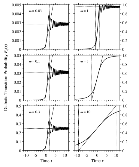
FIG. 1.: The time evolution of the diabatic transition probability $P_{\rm d}(\tau)$ (thick curve) for six values of the coupling $\omega$ – from $\omega=0.03$ (small) to $\omega=10$ (large). In each figure, the horizontal dashed line shows the asymptotic value $P_{\rm d}(\infty)$, Eq. (9) [for $\omega=3$ and 10, it coincides with the axis $P_{\rm d}(\tau)=1$]. The two vertical dashed lines display the jump region, whose beginning is defined by the crossing of the tangent to $P_{\rm d}(\tau)$ at $\tau=0$ (shown by a slanted solid line) with the zero line, whereas its end is defined by the crossing of the tangent with the $P_{\rm d}(\infty)$ line.

The time evolution of $P_{\rm d}(\tau)$ before and after the crossing is well approximated by the formulas [5]

$$P_{\rm d}(\tau<0)\approx\frac{1}{2}+\frac{\tau}{2\sqrt{\tau^{2}+\omega^{2}}},$$ (24)

$$P_{\rm d}(\tau>0)\approx\frac{1}{2}+\left(\frac{1}{2}-e^{-\pi\omega^{2}}\right)\frac{\tau}{\sqrt{\tau^{2}+\omega^{2}}}$$ (25)

$$\qquad\qquad-e^{-\pi\omega^{2}/2}\sqrt{1-e^{-\pi\omega^{2}}}\frac{\omega}{\sqrt{\tau^{2}+\omega^{2}}}\cos\xi(\tau),$$ (26)

valid for $\tau^{2}+\omega^{2}\gtrsim 1$. The phase $\xi(\tau)$ is given by

$$\xi(\tau)=-\frac{\omega^{2}}{2}+\omega^{2}\ln\left[\frac{1}{\sqrt{2}}\left(\tau+\sqrt{\tau^{2}+\omega^{2}}\right)\right]$$ (27)

$$\qquad\qquad+\tau\sqrt{\tau^{2}+\omega^{2}}+\frac{\pi}{4}+\arg\Gamma\left(1-\frac{1}{2}i\omega^{2}\right).$$ (28)

B Jump time

The attempt to define the jump time in a simple and unambiguous manner quickly comes across some difficulties. First of all, it is not obvious how to define the initial time of the transition, because $P_{\rm d}(\tau)$ is nonzero for any finite time. A reasonable choice seems to be the time when the rising transition probability $P_{\rm d}(\tau)$ first equals $\varepsilon P_{\rm d}(\infty)$, where $\varepsilon$ is a suitably chosen small positive number ($\varepsilon\ll 1$). It is even less obvious how to define the final time of the transition in a way that applies to both small and large coupling. One possible choice, used by Lim and Berry [7], is to take the time at which the upper envelope of the oscillations [obtained by setting $\cos\xi(\tau)=-1$ in Eq. (25)] touches unity. However, this idea does not apply for small $\omega$, because then the upper envelope never touches unity. Another possibility is to take the time at which $P_{\rm d}(\tau)$ crosses its asymptotic value $P_{\rm d}(\infty)$ for the first time. However, this is appropriate for small $\omega$ only, because for large $\omega$ (when the oscillations are strongly damped), the crossover takes place at exponentially large times, although $P_{\rm d}(\tau)$ comes very close to $P_{\rm d}(\infty)$ much earlier. Alternatively, one can take the time when $P_{\rm d}(\tau)$ first equals the value $(1-\varepsilon)P_{\rm d}(\infty)$, which is reasonable and consistent with the $\varepsilon$-definition of the initial time discussed above, but leads to a rather complicated expression. I propose here a more elegant and simple solution, which applies to any $\omega$ and provides similar results as the $\varepsilon$-approach. I define the jump time as

$$\tau_{\rm d}^{\rm jump}=\frac{P_{\rm d}(\infty)}{P_{\rm d}^{\prime}(0)}.$$ (29)

This definition is based upon the geometrical meaning of the derivative as the slope of the function at the point of calculation. It provides good results when applied to the most frequently used smooth functions that rise monotonically from 0 to 1, e.g. $f(x)=\frac{1}{2}(1+{\rm tanh}x)$ and $f(x)=\frac{1}{2}(1+x/\sqrt{x^{2}+1})$, typically providing the interval where the function rises from about $0.10-0.15$ to about $0.85-0.90$. By using the exact values of $P_{\rm d}(\infty)$ and $P_{\rm d}^{\prime}(0)$ from Eqs. (9) and (13), we obtain

$$\tau_{\rm d}^{\rm jump}=\frac{\sqrt{1-e^{-\pi\omega^{2}}}}{\omega\cos\chi(\omega)}.$$ (30)

It follows from Eqs. (21) and (22) that

$$\tau_{\rm d}^{\rm jump}\approx\sqrt{2\pi},\qquad(\omega^{2}\ll 1),$$ (32)

$$\tau_{\rm d}^{\rm jump}\approx 2\omega,\qquad(\omega^{2}\gg 1).$$ (33)

In other words, the jump time is proportional to $\omega$ at large $\omega$ while it is nearly constant for small $\omega$. Thus, Eqs. (32) and (33) confirm the scaling properties found in [4] for the extreme cases of small and large $\omega$.

This behavior of the jump time for small and large $\omega$ can be explained from Eqs. (24) and (25), which provide $P_{\rm d}(\tau<0)$ and $P_{\rm d}(\tau>0)$, and from the Taylor expansion of $P_{\rm d}(\tau)$ around $\tau=0$, obtained by using the derivatives (10). It can easily be shown that for large $\omega$, $P_{\rm d}(\tau)$ depends on the ratio $\tau/\omega$ only which means that $\tau_{\rm d}^{\rm jump}\propto\omega$. For small $\omega$, the normalized transition probability $P_{\rm d}(\tau)/P_{\rm d}(\infty)$ depends on $\tau$ only, which can indeed be seen in Fig. 1 for $\omega=0.03$, 0.1 and 0.3; hence, $\tau_{\rm d}^{\rm jump}$ must not depend on $\omega$.

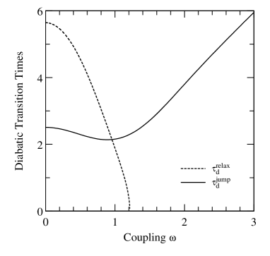
FIG. 2.: The jump time (30) and the relaxation time (34) (for $\varepsilon=0.1$) of the diabatic transition probability, plotted against the dimensionless coupling $\omega\equiv\Omega/\beta$.

C Relaxation time

As Eq. (25) shows, the amplitude of the oscillations in $P_{\rm d}(\tau>0)$ vanishes as $\tau^{-1}$ at large positive times. I define the relaxation time $\tau_{\rm d}^{\rm relax}$ as the time it takes to damp the oscillation amplitude to the (small) value $\varepsilon P_{\rm d}(\infty)$, where $\varepsilon\ll 1$. By using Eq. (25), we find

$$\tau_{\rm d}^{\rm relax}\approx\omega\sqrt{\frac{1}{\varepsilon^{2}\left(e^{\pi\omega^{2}}-1\right)}-1}.$$ (34)

The square root is real only for $\pi\omega^{2}\leqq\ln(1/\varepsilon^{2}+1)$. This inequality imposes an upper limit of $\omega$, above which the oscillation amplitude is never larger than $\varepsilon P_{\rm d}(\infty)$. For $\varepsilon=0.1$, this limit is $\omega\lesssim 1.21$.

The diabatic jump time (30) and the relaxation time (34) (with $\varepsilon=0.1$) are displayed in Fig. 2.

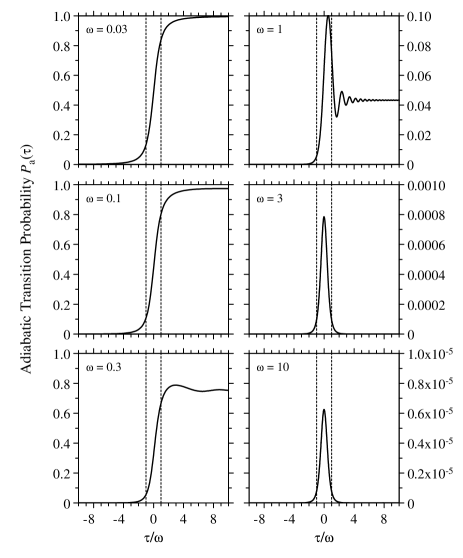
FIG. 3.: The adiabatic transition probability evolution $P_{\rm a}(\tau)$ (solid curve) plotted against the scaled time $\tau/\omega$ for the same six values of the coupling $\omega$ as in Fig. 1 – from $\omega=0.03$ (small) to $\omega=10$ (large). The two vertical dashed lines in each figure display the interval $-\omega\leqq\tau\leqq\omega$, which provides approximately the jump region for $\omega\lesssim 1$.

IV Transition times in the adiabatic basis

A Time evolution of the transition probability

The time evolution of the adiabatic transition probability $P_{\rm a}(\tau)$ is shown in Fig. 3 for the same six values of the coupling $\omega$ as in Fig. 1 – from 0.03 (small) to 10 (large). There are two distinct types of evolution. For small $\omega$, $P_{\rm a}(\tau)$ behaves as the diabatic transition probability $P_{\rm d}(\tau)$ in Fig. 1. For large $\omega$, $P_{\rm a}(\tau)$ rises from zero at $-\infty$ to its maximum near the crossing ($\tau=0$) and then decreases to its exponentially small asymptotic value $P_{\rm a}(\infty)=e^{-\pi\omega^{2}}$ [11]. The small-$\omega$ case can be treated in the same manner as in the diabatic basis, while the large-$\omega$ case requires a more carefull analysis.

The time evolution of the adiabatic transition probability before and after the crossing is approximated by the formulas

$$P_{\rm a}(\tau<0)\approx\frac{\omega^{2}}{16(\tau^{2}+\omega^{2})^{3}},$$ (36)

$$P_{\rm a}(\tau>0)\approx e^{-\pi\omega^{2}}+\left(1-2e^{-\pi\omega^{2}}\right)\frac{\omega^{2}}{16\left(\tau^{2}+\omega^{2}\right)^{3}}$$ (37)

$$\qquad+e^{-\pi\omega^{2}/2}\sqrt{1-e^{-\pi\omega^{2}}}\frac{\omega}{2\left(\tau^{2}+\omega^{2}\right)^{\frac{3}{2}}}\sin\xi(\tau),$$ (38)

valid for $\tau^{2}+\omega^{2}\gtrsim 1$. The phase $\xi(\tau)$ is given by Eq. (27). Equations (IV A), which are new, can be derived from Eq. (7) in the same manner as Eqs. (1) have been derived from Eq. (4) in [5], but by keeping more terms in the large-argument-and-large-order asymptotic expansions [12] of the parabolic cylinder functions in Eq. (7).

B Jump time

1 Small $\omega$

For small $\omega$, the transition probability evolution resembles that in the diabatic basis. Hence, I define the jump time $\tau_{\rm a}^{\rm jump}$ in the same way as Eq. (29),

$$\tau_{\rm a}^{\rm jump}=\frac{P_{\rm a}(\infty)}{P_{\rm a}^{\prime}(0)}.$$ (39)

By using Eqs. (10) and (17) we find that

$$\tau_{\rm a}^{\rm jump}=2\omega e^{-\pi\omega^{2}/2}\approx 2\omega,\qquad(\omega^{2}\ll 1).$$ (40)

Hence, for small $\omega$, the jump time in the adiabatic basis is proportional to $\omega$, as expected.

2 Large $\omega$

For large $\omega$, I define the initial time of the transition as the time $\tau_{\rm a}^{\rm jump,i}<0$ at which $P_{\rm a}(\tau)=\varepsilon P_{\rm a}(\infty)$, where $\varepsilon$ is a suitably chosen small number. It follows from Eq. (36) that

$$\tau_{\rm a}^{\rm jump,i}\approx-\omega\sqrt{\left(\frac{e^{\pi\omega^{2}}}{16\varepsilon\omega^{4}}\right)^{\frac{1}{3}}-1}.$$ (41)

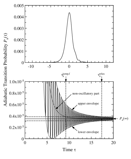
FIG. 4.: The time evolution of the adiabatic transition probability $P_{\rm a}(\tau)$ for $\omega=2$. The upper figure displays the region around the crossing ($\tau=0$). The lower figure gives an expanded view of the region after the crossing, which shows the upper and lower envelopes of the oscillations and the non-oscillatory part of $P_{\rm a}(\tau)$ (short-line dashed curves). The horizontal solid line depicts the asymptotic value $P_{\rm a}(\infty)$, whereas the two horizontal dashed lines above and below it show the values $(1+\varepsilon)P_{\rm a}(\infty)$ and $(1-\varepsilon)P_{\rm a}(\infty)$, respectively, with $\varepsilon=0.1$. The two vertical dashed lines show the final time of the jump $\tau_{\rm a}^{\rm jump,f}$ [defined by the crossing of the non-oscillatory part of $P_{\rm a}(\tau)$ with the $(1+\varepsilon)P_{\rm a}(\infty)$-line] and the relaxation time $\tau_{\rm a}^{\rm relax}$ [defined by the time when the oscillation amplitude gets smaller than $\varepsilon P_{\rm a}(\infty)$].

To define the final time of the jump $\tau_{\rm a}^{\rm jump,f}>0$, I first remark that as $\tau$ increases after the crossing, the non-oscillatory part of the transition probability (37) approaches the asymptotic value $P_{\rm a}(\infty)$ from above [because for $e^{\pi\omega^{2}}>2$, i. e., for $\omega\gtrsim 0.47$, the second term in Eq. (37) is positive]. Hence, I define $\tau_{\rm a}^{\rm jump,f}$ as the time at which the non-oscillatory part of $P_{\rm a}(\tau)$ is equal to $(1+\varepsilon)P_{\rm a}(\infty)$. An illustration of this definition is shown in Fig. 4. A simple calculation gives

$$\tau_{\rm a}^{\rm jump,f}\approx\omega\sqrt{\left(\frac{e^{\pi\omega^{2}}-2}{16\varepsilon\omega^{4}}\right)^{\frac{1}{3}}-1}.$$ (42)

The total jump time is

$$\tau_{\rm a}^{\rm jump}=\tau_{\rm a}^{\rm jump,f}-\tau_{\rm a}^{\rm jump,i}.$$ (43)

For $\omega^{2}\gg 1$, we have

$$\tau_{\rm a}^{\rm jump}\approx\left(\frac{4}{\varepsilon}\right)^{\frac{1}{6}}\omega^{\frac{1}{3}}e^{\pi\omega^{2}/6},\quad(\omega^{2}\gg 1).$$ (44)

Thus, for large $\omega$, the transition time in the adiabatic basis is not proportional to $\omega$, but it rather increases exponentially. This behavior can be explained by the fact that for large $\omega$, $P_{\rm a}(\infty)$ ($=e^{-\pi\omega^{2}}$) is exponentially small and then the population changes in the slowly vanishing wings of the non-adiabatic coupling $\vartheta^{\prime}(\tau)$ [see Eq. (6)] are non-negligible compared to $P_{\rm a}(\infty)$.

C Relaxation time

As Eq. (37) shows, at large positive times the amplitude of the oscillations, that appear in $P_{\rm a}(\tau)$ after the crossing, vanishes as $\tau^{-3}$. The relaxation time $\tau_{\rm a}^{\rm relax}$ is defined in the same way as in the diabatic basis – as the time it takes to damp the oscillation amplitude to the (small) value $\varepsilon P_{\rm a}(\infty)$. By using Eq. (37), we find

$$\tau_{\rm a}^{\rm relax}\approx\omega\sqrt{\left(\frac{e^{\pi\omega^{2}}-1}{4\varepsilon^{2}\omega^{4}}\right)^{\frac{1}{3}}-1}.$$ (45)

For small and large $\omega$, this equation reduces to

$$\tau_{\rm a}^{\rm relax}\approx\left(\frac{\pi}{4\varepsilon^{2}}\right)^{\frac{1}{6}}\omega^{\frac{2}{3}},\qquad(\omega^{2}\ll 1),$$ (47)

$$\tau_{\rm a}^{\rm relax}\approx\left(\frac{1}{2\varepsilon}\right)^{\frac{1}{3}}\omega^{\frac{1}{3}}e^{\pi\omega^{2}/6},\qquad(\omega^{2}\gg 1).$$ (48)

A comparison of Eqs. (34) and (47) shows that for small $\omega$, $\tau_{\rm d}^{\rm relax}\gg\tau_{\rm a}^{\rm relax}$. This is explained by the fact that the oscillation amplitude of $P_{\rm a}(\tau)$ vanishes as $\tau^{-3}$, i. e., much faster than that of $P_{\rm d}(\tau)$ which vanishes as $\tau^{-1}$. In contrast, for large $\omega$, we have $\tau_{\rm a}^{\rm relax}\gg\tau_{\rm d}^{\rm relax}\approx 0$, which follows from the fact that the reference value in the diabatic basis is $P_{\rm d}(\infty)=1-e^{-\pi\omega^{2}}\approx 1$, while the reference value in the adiabatic basis is $P_{\rm a}(\infty)=e^{-\pi\omega^{2}}\ll 1$.

The adiabatic jump time $\tau_{\rm a}^{\rm jump}$ and the relaxation time $\tau_{\rm a}^{\rm relax}$ (for $\varepsilon=0.1$) are displayed in Fig. 5. Note that, as follows from Eqs. (44) and (48), the ratio between the jump and relaxation times at large $\omega$ is constant, $\tau_{\rm a}^{\rm jump}/\tau_{\rm a}^{\rm relax}\approx(16\varepsilon)^{\frac{1}{6}}$, i. e., they are almost equal for $\varepsilon=0.1$. In the evolution picture (Fig. 4), however, the relaxation ends later than the jump, because the jump time is calculated from $\tau=\tau_{\rm a}^{\rm jump,i}<0$, while the relaxation time is calculated from the crossing ($\tau=0$).

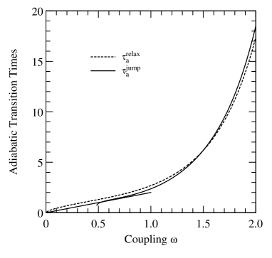
FIG. 5.: The jump and relaxation times of the adiabatic transition probability, plotted against the dimensionless coupling $\omega\equiv\Omega/\beta$. The small-$\omega$ jump time (40) is shown by the solid line in the range $0\leqq\omega\leqq 1$, whereas the large-$\omega$ jump time (43) is shown by the solid curve for $\omega\geqq 0.5$. Note that the small-$\omega$ and large-$\omega$ formulas agree well for $0.5<\omega<1$. The relaxation time (45) is plotted by a dashed curve.

V Summary of the results and conclusions

In the present paper, I have calculated various transition times in the Landau-Zener model. I have emphasized the differences between the transition times in the diabatic and adiabatic bases, and between the jump time and the relaxation time. The jump time is the time for which the transition probability rises to the region of its asymptotic value $P(\infty)$. The relaxation time is the time for which the amplitude of the oscillations, which appear in the transition probability after the crossing, is damped below the (small) value $\varepsilon P(\infty),\ (\varepsilon\ll 1)$. These transition times have been calculated by using the exact values of the transition probabilities and their derivatives at the crossing point as well as approximations to the transition probabilities evolutions derived in [5] and here.

The results for the jump time in the diabatic basis $\tau_{\rm d}^{\rm jump}$ confirm the scaling properties found by Mullen et al [4] in the limits of small and large coupling $\omega$, i. e., for large $\omega$, $\tau_{\rm d}^{\rm jump}$ is proportional to $\omega$, whereas for small $\omega$, $\tau_{\rm d}^{\rm jump}$ is constant. The jump time in the adiabatic basis $\tau_{\rm a}^{\rm jump}$ has a rather different dependence on $\omega$. The seemingly obvious conclusion that $\tau_{\rm a}^{\rm jump}$ should be proportional to $\omega$ (because the non-adiabatic coupling is a Lorentzian function of time with a width of $2\omega$ and the energies of the two adiabatic states have an avoided crossing with the same duration) turns out to be correct for small $\omega$ only, while for large $\omega$, $\tau_{\rm a}^{\rm jump}$ increases exponentially.

The relaxation times in the two bases, $\tau_{\rm d}^{\rm relax}$ and $\tau_{\rm a}^{\rm relax}$, also show rather different dependences on $\omega$. The diabatic relaxation time $\tau_{\rm d}^{\rm relax}$ is a decreasing function of $\omega$ and it vanishes above certain $\omega$ ($\approx 1.2$), whereas the adiabatic relaxation time $\tau_{\rm a}^{\rm relax}$ is an exponentially increasing function of $\omega$.

It should be pointed out that the transition times obtained in this work refer to the transition probabilities $P_{\rm d}(\tau)$ and $P_{\rm a}(\tau)$. These may differ from the transition times for the probabilities of no transition, $1-P_{\rm d}(\tau)$ and $1-P_{\rm a}(\tau)$, particularly those times which are linked to the values of the probabilities at $\tau\rightarrow\infty$.

The present paper has dealt with the transition times in the diabatic and adiabatic bases only, which are the most frequently used bases in practical applications of the LZ model. It has been shown by Berry and Lim [7, 13] in their superadiabatic treatment of quantum evolution that the transition time is shortest and the oscillations in the corresponding transition probability are minimal in the optimal superadiabatic basis.

In conclusion, the transition times obtained in this paper provide simple criteria for estimating the applicability of the Landau-Zener model to various cases of level crossings and avoided crossings.

A Numerical integration of the Landau-Zener problem

1 Diabatic basis

Since in the LZ model (2) the coupling does not vanish at infinity and the detuning approaches infinity very slowly, the numerical integration of Eq. (1) is not a trivial problem, particularly when high accuracy is required. The straightforward way of integrating Eq. (1) is to start at a certain large negative time and propagate the solution towards $+\infty$. However, a finite initial time $\tau_{\rm i}$ generates spurious oscillations with an amplitude proportional to $(\tau_{\rm i}^{2}+\omega^{2})^{-\frac{1}{2}}$ [5] and one has to take a very large $\tau_{\rm i}$ in order to achieve a good accuracy in $P_{\rm d}(\tau)$, which is very expensive in terms of computation time. An alternative and much more efficient solution to this problem has been proposed in [5], which is summarized here for the reader’s convenience. The transition probability is derived from the equation for the population inversion $w_{\rm d}(\tau)\equiv 2P_{\rm d}(\tau)-1$ (derived from the optical Bloch equations [6]),

$$\tau w_{\rm d}^{\prime\prime\prime}-w_{\rm d}^{\prime\prime}+4\tau(\omega^{2}+\tau^{2})w_{\rm d}^{\prime}-4\omega^{2}w_{\rm d}=0,$$ (A1)

rather than from Eq. (1). The integration starts at $\tau=0$ and the solution is propagated towards the desired (positive or negative) time. The initial conditions are found by identifying the terms in the Taylor expansion of $P_{\rm d}(\tau)$ around $\tau=0$ [obtained by using the power series expansions of the parabolic cylinder functions in Eq. (4)] with the derivatives of $P_{\rm d}(\tau)$ at $\tau=0$. The initial values needed to start a Runge-Kutta algorithm, are

$$w_{\rm d}(0)=-e^{-\pi\omega^{2}/2}$$ (A3)

$$w_{\rm d}^{\prime}(0)=2\omega\sqrt{1-e^{-\pi\omega^{2}}}\cos\chi$$ (A4)

$$w_{\rm d}^{\prime\prime}(0)=4\omega^{2}e^{-\pi\omega^{2}/2}$$ (A5)

$$w_{\rm d}^{\prime\prime\prime}(0)=4\omega\sqrt{1-e^{-\pi\omega^{2}}}(\sin\chi-2\omega^{2}\cos\chi)$$ (A6)

where $\chi(\omega)$ is given by Eq. (19).

2 Adiabatic basis

A similar numerical method, which is new and complements the one described above for the diabatic basis [5], can be used to obtain the transition probability $P_{\rm a}(\tau)$ in the adiabatic basis and it has similar advantages. It turns out convenient to use the angle $\vartheta\equiv\frac{1}{2}\arctan(\omega/\tau)$, rather than the time $\tau$, as an independent variable. The equation for the population inversion $W_{\rm a}[\vartheta(\tau)]=w_{\rm a}(\tau)\equiv 2P_{\rm a}(\tau)-1$ has the form

$$W_{\rm a}^{\prime\prime\prime}+6\cot 2\vartheta\ W_{\rm a}^{\prime\prime}+4[4\omega^{4}(\cot^{2}2\vartheta+1)^{3}+1]W_{\rm a}^{\prime}$$ (A7)

$$+24\cot 2\vartheta\ W_{\rm a}=0,$$ (A8)

where a prime now means $d/d\vartheta$. The initial values of $W_{\rm a}(\vartheta)$ and its derivatives at $\vartheta=\pi/4$ (i. e., at $\tau=0$), needed to start a Runge-Kutta algorithm, are

$$W_{\rm a}(\pi/4)=-\sqrt{1-e^{-\pi\omega^{2}}}\sin\chi,$$ (A10)

$$W_{\rm a}^{\prime}(\pi/4)=-2e^{-\pi\omega^{2}/2},$$ (A11)

$$W_{\rm a}^{\prime\prime}(\pi/4)=4\sqrt{1-e^{-\pi\omega^{2}}}\left(\sin\chi-2\omega^{2}\cos\chi\right),$$ (A12)

$$W_{\rm a}^{\prime\prime\prime}(\pi/4)=8\left(4\omega^{4}+1\right)e^{-\pi\omega^{2}/2}.$$ (A13)

with $\chi(\omega)$ given by Eq. (19).

REFERENCES

- [1] electronic address: vitanov@rock.helsinki.fi
- [2] L. D. Landau, Physik Z. Sowjetunion 2, 46 (1932).
- [3] C. Zener, Proc. Roy. Soc. Lond. A 137, 696 (1932).
- [4] K. Mullen, E. Ben-Jacob, Y. Gefen, and Z. Schuss, Phys. Rev. Lett. 62, 2543 (1989).
- [5] N. V. Vitanov and B. M. Garraway, Phys. Rev. A 53, 4288 (1996), erratum Phys. Rev. A 54, 5458 (1996).
- [6] B. W. Shore, The Theory of Coherent Atomic Excitation, vol. I (Wiley, New York, 1990).
- [7] R. Lim and M. V. Berry, J. Phys. A 24, 3255 (1991).
- [8] A. Erdélyi, W. Magnus, F. Oberhettinger, F. G. Tricomi, Higher Transcendental Functions, vol. II (McGraw-Hill, New York, 1953).
- [9] M. Abramowitz and I. A. Stegun (editors), Handbook of Mathematical Functions (Dover, New York, 1964).
- [10] K. M. Abadir, J. Phys. A 26, 4059 (1993).
- [11] This behavior can be deduced more rigorously from Eqs. (10) and (16), which show that for , , and from Eqs. (17), (18) and (22), which give and , that indicates a maximum of near .
- [12] F. W. J. Olver, J. Res. Nat. Bur. Stand. 63B, 131 (1959).
- [13] M. V. Berry, Proc. R. Soc. London A 429, 61 (1990).