A new entanglement measure induced by the Hilbert-Schmidt norm

Abstract

In this letter we discuss a new entanglement measure. It is based on the Hilbert-Schmidt norm of operators. We give an explicit formula for calculating the entanglement of a large set of states on $\mathbb{C}^{2}\otimes\mathbb{C}^{2}$. Furthermore we find some relations between the entanglement of relative entropy and the Hilbert-Schmidt entanglement. A rigorous definition of partial transposition is given in the appendix.

1 Introduction

Quantum information processing has received a considerable interest in the last years, induced by the possibility of teleporting an unknown quantum state and building a quantum computer. Also new questions on the relation of quantum and classical physics arise in this context. The feature which makes quantum computation more efficient than classical computation and allows teleportation is entanglement. Therefore there is also an increasing interest in quantifying entanglement [1]. Our letter considers the quantification by introducing a new entanglement measure.

For pure states on the tensor product of two Hilbert spaces a measure is given by the entanglement of entropy. Let ${\mathcal{T}}$ be the set of states on the tensor product of two Hilbert spaces ${\mathcal{H}}_{1}\otimes{\mathcal{H}}_{2}$, i.e. the set of all positive trace class operators with trace 1. For a pure state $\sigma\in{\mathcal{T}}$, the entanglement of entropy $E(\sigma)$ is given by

$$E(\sigma):=-\mbox{tr}\;(\sigma_{1}\log_{2}\sigma_{1})=-\mbox{tr}\;(\sigma_{2}\log_{2}\sigma_{2})=-\sum_{i}|\alpha_{i}|^{2}\log_{2}|\alpha_{i}|^{2}$$ (1)

where $\sigma_{i}=\mbox{tr}_{i}\;\sigma,i=1,2,$ are the partial traces taken in the Hilbert spaces ${\mathcal{H}}_{i}$ and $\alpha_{i}$ are the Schmidt coefficients of $\sigma$ (cp. [2]).

Considering mixed states, the situation is more complicated. Several entanglement measures have been defined in this case, e.g. the entanglement of creation [3] and the entanglement of distillation [3]. Here we follow an idea of Vedral et al. [1], based on measuring the distance between states in the quantum mechanical state space. The set of disentangled states ${\mathcal{D}}$ is usually considered as the set of all states which can be written as convex combinations of pure tensor states:

$${\mathcal{D}}:=\{\rho\in{\mathcal{T}}\;|\;\rho=\sum_{i}p_{i}\rho^{(1)}_{i}\otimes\rho^{(2)}_{i},\sum_{i}p_{i}=1,\rho^{(k)}_{i}\in{\mathcal{T}}({\mathcal{H}}_{i}),k=1,2\}.$$

The general idea of Vedral et al. [1] to quantify the amount of entanglement of a state $\sigma\in{\mathcal{T}}\setminus{\mathcal{D}}$ is to define a distance of $\sigma$ to the set ${\mathcal{D}}$, so that the entanglement $E$ of $\sigma$ is given by

$$E(\sigma)=\min_{\rho\in{\mathcal{D}}}D(\sigma||\rho).$$ (2)

Here $D$ is any measure of distance between the density matrices $\rho$ and $\sigma$, not necessarily a distance in the metrical sense. There are several possibilities to define such a distance. One example is the relative entropy $S(\sigma||\rho)$, given by

$$S(\sigma||\rho):=\mbox{tr}\;(\sigma\log_{2}\sigma-\sigma\log_{2}\rho),$$

discussed in [1, 4]. Another example is to take the Bures metric as distance [4].

As a measure of distance we discuss in this letter the Hilbert-Schmidt norm. The Hilbert-Schmidt norm is defined by

$$\|A\|_{\mathrm{HS}}^{2}:=\mbox{tr}\;(A^{*}A),$$

for all Hilbert-Schmidt operators on $\mathcal{H}={\mathcal{H}}_{1}\otimes{\mathcal{H}}_{2}$, i.e. for all operators if $\dim\mathcal{H}<\infty$. We therefore define the Hilbert-Schmidt entanglement (HS entanglement) $E_{\mathrm{HS}}$ of a state $\sigma$ by

$$E_{\mathrm{HS}}(\sigma):=\min_{\rho\in{\mathcal{D}}}\|\rho-\sigma\|^{2}_{\mathrm{HS}}.$$

The choice of the squared distance instead of $\|\rho-\sigma\|_{\mathrm{HS}}$ is motivated by the fact that it is easier in calculations and justified because they are equivalent to each other.

There are several requirements every measure of entanglement $E$ should satisfy (see e.g. [1, 4] for a more detailed discussion):

1. $E(\sigma)=0$ for all $\sigma\in{\mathcal{D}}$.

2. $E(\sigma)=E(U_{1}\otimes U_{2}\sigma U_{1}^{*}\otimes U_{2}^{*})$ for all unitary operators $U_{i}\in{\mathcal{H}}_{i},i=1,2,$ i.e. the measure is invariant under local unitary operations.

3. The measure $E$ does not increase under local general measurements and classical communication, i.e. for every completely positive trace-preserving map $\Theta:{\mathcal{T}}\to{\mathcal{T}}$ we have $E(\Theta\sigma)\leq E(\sigma)$.

Of course every measure of entanglement defined by eq. (2) trivially fulfils the first requirement. It can be seen as follows that condition (2) is satisfied: With $U=U_{1}\otimes U_{2}$, we have

$$E(U\sigma U^{*}) = \min_{\rho\in{\mathcal{D}}}\|\rho-U\sigma U^{*}\|^{2}$$

$$= \min_{\rho\in{\mathcal{D}}}\mbox{tr}\;(\rho^{2}-2\rho U\sigma U^{*}+U\sigma^{2}U^{*})$$

$$= \min_{\tilde{\rho}\in{\mathcal{D}}}\mbox{tr}\;(\tilde{\rho}^{2}-2\tilde{\rho}\sigma+\sigma^{2})$$

$$= \min_{\rho\in{\mathcal{D}}}\|\rho-\sigma\|^{2}=E(\sigma),$$

where we set $\tilde{\rho}=U^{*}\rho\,U\in{\mathcal{D}}$. To show that the third condition is fulfilled we apply a theorem of Lindblad [5].

Theorem 1

Let $\Phi:B({\mathcal{H}})\to B({\mathcal{H}})$ be a positive mapping. Then

$$\|\Phi\|\leq 1,\quad\mathrm{tr}\;(\Phi A)=\mathrm{tr}\;A,\quad\forall A\in{\mathcal{T}}({\mathcal{H}})$$

$$\Longleftrightarrow\quad f(\Phi A)\leq f(A),\quad\forall f\;\mathrm{convex},\quad A\in{\mathcal{T}}({\mathcal{H}}).$$

Now since $\sigma\to E(\sigma)$ is a convex function, we conclude that $E(\Theta\sigma)\leq E(\sigma)$.

2 The HS-entanglement of some special states

The use of geometric distance in the real vector space of selfadjoint matrices as a measure of entanglement gives us the possibility to see the point of minimal distance in ${\mathcal{D}}$ (here referred to as basepoint) for some important cases easily. Recall that the distance of an arbitrary point outside a convex and compact set ${\mathcal{C}}$ to this set is the closest distance to any orthogonal projection of the point onto the (nontrivial) faces of ${\mathcal{C}}$ (A face $\mathcal{C}$ of a convex set $K$ is a convex subset of $K$ such that $\phi=\lambda\phi_{1}+(1-\lambda)\phi_{2}$ for $\phi\in\mathcal{C}$, $\phi_{1,2}\in K$ and $0<\lambda<1$ imply $\phi_{1,2}\in\mathcal{C}$. A face consisting of one point is an extremal point of $K$. The trivial faces are the set $K$ itself and the empty set). The first set of states to be investigated are, traditionally, the so-called Bell-states on ${\mathcal{H}}=\mathbb{C}^{2}\otimes\mathbb{C}^{2}$. These are expected to be maximally entangled for reasonable measures of entanglement. This proves to be true also in this case.

Let us denote the basis of Bell-vectors corresponding to the natural basis $\{|0\rangle,|1\rangle\}$ of $\mathbb{C}^{2}$ by $\psi_{1}=1/\sqrt{2}(|0\rangle|0\rangle\!+\!|1\rangle|1\rangle)$, $\psi_{2}=1/\sqrt{2}(|0\rangle|0\rangle\!-\!|1\rangle|1\rangle)$, $\psi_{3}=1/\sqrt{2}(|0\rangle|1\rangle\!+\!|1\rangle|0\rangle)$ and $\psi_{4}=1/\sqrt{2}(|0\rangle|1\rangle\!-\!|1\rangle|0\rangle)$. Furthermore $\Psi_{i}$ denotes the one-dimensional projector on the vector $\psi_{i}$ (Bell-state) and $\Phi_{ij}=1/2(\Psi_{i}+\Psi_{j})$ the equally weighted mixture of $\Psi_{i}$ and $\Psi_{j}$. For a given Bell-state $\Psi_{i}$ a Werner-state [6] is given by $W_{\psi_{i},\epsilon}=1/4(1-\epsilon)\mathbf{1}+\epsilon\Psi_{i}$, with $\epsilon\in[0,1]$. We can now formulate the following proposition, which gives the entanglement of the Bell-states and arbitrary mixtures of orthogonal Bell-states:

Proposition 2

For an arbitrary mixture of orthogonal Bell-states

$$\sigma=\lambda_{i}\Psi_{i}+\sum_{j\neq i}\lambda_{j}\Phi_{ij},$$

where $\lambda_{i}\geq 0$ and $\sum\lambda_{i}=1$, the basepoint in ${\mathcal{D}}$ is given by

$$\tilde{\sigma}=\lambda_{i}W_{\psi_{i},1/3}+\sum_{j\neq i}\lambda_{j}\Phi_{ij}$$

and we find:

$$E_{\mathrm{HS}}(\sigma)=\lambda_{i}^{2}/3.$$

Before we prove the proposition we give some remarks. Obviously, for a given index $i$ we have found the entanglement of the Bell-state $\Psi_{i}$ and all the states in the tetrahedron spanned by this Bell-state and the three mixtures $\Phi_{ij}$. The complement of these four tetrahedra in the larger tetrahedron of all mixtures of the four Bell-states is just the octahedron spanned by the six disentangled states $\Phi_{ij}$ for $i\neq j$, which is therefore a subset of the set ${\mathcal{D}}$. The fact that the states $\Phi_{ij}$ are in fact disentangled can be seen easily by either decomposition of $\Phi_{ij}$ into disentangled projectors or partial transposition. Thus all the mixtures of the four given Bell-states are covered by the proposition. Proof of the proposition We prove the fact that the suggested basepoint $\tilde{\sigma}$ is correct, by showing that the derivative of the function $f(\rho)=||\sigma-\rho||^{2}$ is non-negative at $\tilde{\sigma}$ in any direction leading into the convex set ${\mathcal{D}}$. Such a directional derivative can be computed by using a parameterised line

$$\rho(s)=(1-s)\,\tilde{\sigma}+s\,\omega,$$

where $\omega$ is an arbitrary element of ${\mathcal{D}}$ and calculating the derivative

$$\frac{d}{ds}f(\rho(s))|_{0} = \lim_{s\to 0}\frac{f(\rho(s))-f(\tilde{\sigma})}{s}$$

$$= \lim_{s\to 0}\frac{1}{s}\operatorname{tr}\bigl{(}(\rho(s)-\sigma)^{2}-(\tilde{\sigma}-\sigma)^{2}\bigr{)}$$

$$= \lim_{s\to 0}\frac{1}{s}\operatorname{tr}\bigl{(}2s(\sigma-\tilde{\sigma})(\tilde{\sigma}-\omega)+s^{2}(\tilde{\sigma}-\omega)^{2}\bigr{)}$$

$$= \operatorname{tr}\bigl{(}2(\sigma-\tilde{\sigma})(\tilde{\sigma}-\omega)\bigr{)}.$$

We see that this derivative is an affine functional of the element $\omega\in{\mathcal{D}}$. Therefore convex combinations of elements in ${\mathcal{D}}$ lead to a convex combination of the result. For that reason it suffices to show non-negativity of the above expression only for $\omega\in\partial_{e}{\mathcal{D}}$, where $\partial_{e}$ denotes extreme points, in other words for disentangled projectors.

Inserting the given expressions for $\sigma$ and $\tilde{\sigma}$ as well as choosing $\omega=P_{\chi}\otimes P_{\xi}$ to be a projector onto the normalised vectors $\chi$ and $\xi$, we get:

$$\frac{d}{ds}f(\rho(s))|_{0} = 2\lambda_{i}\operatorname{tr}\bigl{(}(\Psi_{i}-W_{\psi_{i},1/3})(\lambda_{i}W_{\psi_{i},1/3}+\sum_{j\neq i}\lambda_{j}\Phi_{ij}-P_{\chi}\otimes P_{\xi})\bigr{)}$$

$$= 2\lambda_{i}\bigl{(}\lambda_{i}/2+\sum_{j\neq i}\lambda_{j}/2-\operatorname{tr}(\Psi_{i}P_{\chi}\otimes P_{\xi})-\lambda_{i}/3-\sum_{j\neq i}\lambda_{j}/3$$

$${}+\lambda_{i}/6+\operatorname{tr}(\Psi_{i}P_{\chi}\otimes P_{\xi})/3\bigr{)}$$

$$= 2\lambda_{i}(1-2\operatorname{tr}(\Psi_{i}P_{\chi}\otimes P_{\xi}))/3$$

$$= 2\lambda_{i}(1-2\langle\psi_{i},\chi\otimes\xi\rangle\langle\chi\otimes\xi,\psi_{i}\rangle)/3$$

$$= 2\lambda_{i}(1-2|\langle\chi\otimes\xi,\psi_{i}\rangle|^{2})/3.$$

Since any $\psi_{i}$ is of the form $(|0\rangle\otimes U|0\rangle+|1\rangle\otimes U|1\rangle)/\sqrt{2}$, where $U$ is a unitary transformation, we can write:

$$\frac{d}{ds}f(\rho(s))|_{0} = 2\lambda_{i}(1-|\langle\chi|0\rangle\langle U^{*}\xi|0\rangle+\langle\chi|1\rangle\langle U^{*}\xi|1\rangle|^{2})/3$$

$$= 2\lambda_{i}(1-|\chi_{0}(U^{*}\xi)_{0}+\chi_{1}(U^{*}\xi)_{1}|^{2})/3$$

$$= 2\lambda_{i}(1-|\langle\bar{\chi},U^{*}\xi\rangle|^{2})/3$$

$$\geq 0.$$

The final step is just an application of the Cauchy-Schwartz inequality. ∎ The next class of states we are going to deal with also includes the Bell-states as special case, namely the pure states. Unfortunately, the geometry of the underlying part of the face of ${\mathcal{D}}$ proves to be somewhat more complex. This leads to the fact that pure states admit an easy-to-construct basepoint only under a certain condition, which is stated in the following proposition:

Proposition 3

Let $\phi$ be a vector in $\mathbb{C}^{2}\otimes\mathbb{C}^{2}$, written in its Schmidt-basis as $\phi=a|0\rangle\otimes|0\rangle+b|1\rangle\otimes|1\rangle$ with $a$ and $b$ positive numbers, such that

$$a^{2}\in\bigl{[}\frac{1}{2}-\frac{\sqrt{5}}{6},\frac{1}{2}+\frac{\sqrt{5}}{6}\bigr{]}\quad;\quad b^{2}=1-a^{2}.$$

The basepoint associated to the one-dimensional entangled projector $\sigma$ onto the span of $\phi$ is then given by:

$$\tilde{\sigma}=\sigma-ab(4P_{\psi_{1}}-\mathbf{1})/3,$$

where $P_{\psi_{1}}$ is the Bell-state for $\psi_{1}=|0\rangle|0\rangle+|1\rangle|1\rangle$. The entanglement of $\sigma$ is given by:

$$E_{\mathrm{HS}}(\sigma)=4a^{2}b^{2}/3.$$

[Proof.] The suggested basepoint $\tilde{\sigma}$ has to be shown to lie in ${\mathcal{D}}$, first. According to the Peres criterion [7] it suffices to show that $\tilde{\sigma}$ as well as its partial transpose are positive. A rigorous definition of partial transposition is given in the appendix. In this case $\sigma^{T_{2}}$ (partial transposition of $\sigma$ in the second factor) has exactly one negative eigenvalue, which can be seen by writing:

$$\sigma=a^{2}P_{|0\rangle|0\rangle}+b^{2}P_{|1\rangle|1\rangle}+abP_{+}^{T_{2}}-abP_{-}^{T_{2}},$$

where $P_{+}$ denotes the projector onto $\mbox{span}(|0\rangle|1\rangle+|1\rangle|0\rangle)$ and $P_{-}$ denotes the projector onto $\mbox{span}(|0\rangle|1\rangle-|1\rangle|0\rangle)$. $\tilde{\sigma}$ was found by projecting onto the corresponding plane with eigenvalue zero ($\{\rho:\operatorname{tr}\rho=1\wedge\operatorname{tr}(P_{-}^{T_{2}}\rho)=0\}$), thus:

$$\tilde{\sigma}=(a^{2}-ab/3)P_{|0\rangle|0\rangle}+(b^{2}-ab/3)P_{|1\rangle|1\rangle}+2abP_{+}^{T_{2}}/3.$$

$\tilde{\sigma}^{T_{2}}$ is positive, iff $a^{2}-ab/3>0$ and $b^{2}-ab/3>0$. This yields the condition:

$$a^{2}\in[1/10,9/10].$$

The stronger condition is nevertheless the positivity of $\tilde{\sigma}$ itself. We find that the only possibly negative eigenvalue has to satisfy the following inequality:

$$3-2ab-\sqrt{9a^{4}-14a^{2}b^{2}+9b^{4}} \geq 0$$ (3)

$$(3-2ab)^{2} \geq 9a^{4}-14a^{2}b^{2}+9b^{4}$$

$$12ab \geq 36(a^{2}-a^{4})$$

$$1 \geq 3ab.$$

This inequality is exactly satisfied for $a^{2}$ in the stated interval.

It remains to prove minimality of the distance of the basepoint to the pure state $\sigma$. In the notation of the preceding proof we have to calculate here:

$$\frac{d}{ds}f(\rho(s))|_{0} = \operatorname{tr}\bigl{(}2(\sigma-\tilde{\sigma})(\tilde{\sigma}-\omega)\bigr{)}$$

and show that this expression is non-negative for any disentangled one-dimensional projector $\omega=P_{\xi}\otimes P\chi$.

We find:

$$\operatorname{tr}(\sigma-\tilde{\sigma})\tilde{\sigma} = ab\operatorname{tr}((4P_{\psi_{1}}-\mathbf{1})(\tilde{\sigma}))/3$$

$$= ab(\operatorname{tr}(4P_{\psi_{1}}\tilde{\sigma})-1)/3$$

$$= ab(-4ab+4\operatorname{tr}(P_{\psi_{1}}\sigma)-1)/3$$

$$= ab/3$$

Finally:

$$\frac{d}{ds}f(\rho(s))|_{0} = 2ab[1-\operatorname{tr}((4P_{\psi_{1}}-\mathbf{1})P_{\xi}\otimes P_{\chi}))]/3$$

$$= 2ab(2-4\operatorname{tr}(P_{\psi_{1}}P_{\xi}\otimes P_{\chi}))/3,$$

which is, except for the leading positive factor, the same expression as in the preceding proof and thus non-negative.

The explicit quantity of the entanglement is a pure matter of calculation. ∎

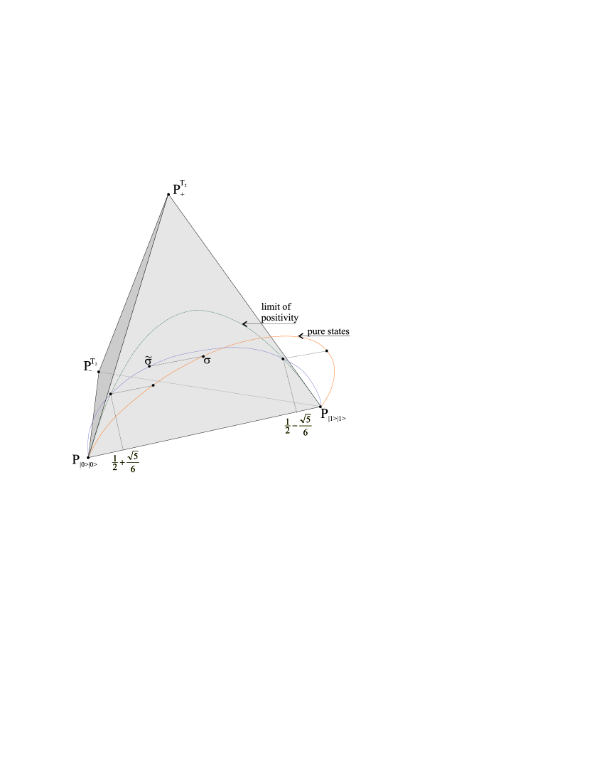
Figure 1: Pure states and their projection: Pure states lie on the marked semicircle and are projected onto the triangle spanned by the three partially transposed projectors in the front. The line formed by the projected semicircle is a segment of an ellipse that intersects the parabola marked as limit of positivity at the two critical Schmidt coefficients. Only the states below this parabola are positive. The projected states above the limit of positivity are therefore not admissible.

For the remaining pure states the calculation of the entanglement is a bit more complicated. For this purpose we first parameterise the parabola that forms the border of the positive elements in the triangle $conv(\{P_{|0\rangle|0\rangle},P_{|1\rangle|1\rangle},P_{+}^{T_{2}}\})$ (see fig. 1):

$$p(s) := s^{2}P_{|0\rangle|0\rangle}+(1-2s+s^{2})P_{|1\rangle|1\rangle}+2(s-s^{2})P_{+}^{T_{2}}$$

It is easy to see that this is a parabola, indeed, and explicit calculation of the eigenvalues shows that the elements have a zero eigenvalue. The idea is now to project onto this parabola, instead of the whole triangle. Finding the minimal distance of the given pure state to the parabola corresponds to minimising the function

$$f(s)=\operatorname{tr}(p(s)-P_{\phi})^{2}$$ (4)

leading to a third order equation in the parameter $s$. Even though rather cumbersome, this case illustrates the problems in finding explicit solutions for entanglement measures. We state the solution here as a conjecture only, and will give the proof elsewhere.

Conjecture 4

Let $\phi$ be a vector in $\mathbb{C}^{2}\otimes\mathbb{C}^{2}$, written in its Schmidt-basis as $\phi=a|0\rangle\otimes|0\rangle+b|1\rangle\otimes|1\rangle$ with $a$ and $b$ positive numbers, such that

$$a^{2}\in\bigl{[}0,\frac{1}{2}-\frac{\sqrt{5}}{6}\bigr{]}\cup\bigl{[}\frac{1}{2}+\frac{\sqrt{5}}{6},1\bigr{]}\quad;\quad b^{2}=1-a^{2}.$$

The basepoint associated to the one-dimensional entangled projector $\sigma$ onto the span of $\phi$ is then given by:

$$t^{2}P_{|0\rangle|0\rangle}+(1-2t+t^{2})P_{|1\rangle|1\rangle}+2(t-t^{2})P_{+}^{T_{2}},$$ (5)

where $t\in\Rset$ is the real solution of the cubic equation

$$-1-ab+b^{2}+(5-a^{2}+2ab-b^{2})t-9t^{2}+6t^{3}=0.$$ (6)

Finally we state a corollary that is independent on the conjecture above:

Corollary 5

The Bell-states, i.e. the projectors associated to vectors of the form $U|0\rangle|0\rangle\otimes V|1\rangle|1\rangle$, where $U$ and $V$ are unitary operators on the single particle Hilbert spaces, are maximally entangled w.r.t the HS-entanglement.

[Proof.] Every pure state has a HS-entanglement less or equal to the Bell-states (which evaluates to $1/3$). This is obvious for those states covered be Prop. 3, as seen by evaluating the explicitly given formula for the entanglement. For those states covered by the conjecture, we find, even if the exact value of the entanglement is unknown, the following inequality:

$$E(P_{\phi}) \leq \operatorname{tr}(P_{\phi}P_{|0\rangle|0\rangle})^{2}$$

$$= 2-2\operatorname{tr}(P_{\phi}P_{|0\rangle|0\rangle})$$

$$= 2-2a^{2}$$

$$\leq 1-\sqrt{5}/3\quad\quad(*)$$

$$\leq 1/3,$$

where $(*)$ is valid for those states with $a^{2}\in[1/2+\sqrt{5}/6,1]$. For those states with $a^{2}\in[0,1/2-\sqrt{5}/6]$ the same argument using $P_{|1\rangle|1\rangle}$ instead of $P_{|0\rangle|0\rangle}$ is valid.

We conclude that mixed states have an entanglement that is less or equal to its most entangled spectral projector (decomposed to dimension one), because the HS-entanglement is a convex function and spectral decomposition of operators in $\mathcal{T}$ is a convex combination. ∎

Remark 6

Obviously not only the pure states, but also the mixture of each of these and their associated basepoint are analysed by our method. Convex combinations of a given state and its basepoint share, of course, the same basepoint. Also, it is easy to see that their entanglement is given by

$$E_{\mathrm{HS}}(\lambda\sigma+(1-\lambda)\tilde{\sigma})=\lambda^{2}E_{\mathrm{HS}}(\sigma).$$ (8)

3 The use of HS-entanglement

The most obvious use of the HS-entanglement is its easy form, which makes an explicit calculation possible by merely knowing the geometric structure of the set of disentangled states. On the other hand it also has the more practical property of yielding useful estimates for other measures of entanglement. As an example we give an inequality connecting the HS-entanglement to the very useful measure based on the relative entropy (referred to as $E_{\mathrm{vN}}$ here).

Proposition 7

For any entangled state $\sigma\in{\mathcal{T}}$ the following inequality holds:

$$E_{\mathrm{vN}}(\sigma)\geq\frac{1}{2\log_{2}2}E_{\mathrm{HS}}(\sigma)$$

[Proof.] We denote the basepoints of $\sigma$ in ${\mathcal{D}}$ w.r.t.  the relative entropy by $\hat{\sigma}$ and w.r.t.  the distance by $\tilde{\sigma}$. We get:

$$E_{\mathrm{vN}}(\sigma) = S(\sigma||\hat{\sigma})$$

$$\geq \frac{1}{2\log_{2}2}||\sigma-\hat{\sigma}||^{2}$$

$$\geq \frac{1}{2\log_{2}2}||\sigma-\tilde{\sigma}||^{2}$$

$$= \frac{1}{2\log_{2}2}E_{\mathrm{HS}}(\sigma),$$

where we used a well-known estimate for the relative entropy (cf. [8, Prop.1.1]), adjusted to the use of $\log_{2}$ instead of $\ln$. ∎

Remark 8

For pure states on the tensor product of two Hilbert spaces the entanglement of relative entropy is given by

$$E_{\mathrm{vN}}(\sigma)=-a^{2}\log_{2}a^{2}-b^{2}\log_{2}b^{2}=-a^{2}\log_{2}a^{2}-(1-a^{2})\log_{2}(1-a^{2})$$

where $a$ and $b$ are the Schmidt coefficients of $\psi$, $\sigma=|\psi\rangle\langle\psi|$ (see Eq. (1)). The Hilbert-Schmidt entanglement gives the same order as this entanglement measure on pure states on $\mathbb{C}^{2}\otimes\mathbb{C}^{2}$, i.e.

$$E_{\mathrm{vN}}(\sigma)\leq E_{\mathrm{vN}}(\rho)\iff E_{\mathrm{HS}}(\sigma)\leq E_{\mathrm{HS}}(\rho)$$ (9)

for pure states $\rho$ and $\sigma$. E.g.  we have shown in Prop. 3, that

$$E_{\mathrm{HS}}(\sigma)=4a^{2}b^{2}/3=4a^{2}(1-a^{2})/3.$$

Considering $E_{\mathrm{vN}}$ and $E_{\mathrm{HS}}$ as functions of $a$, both functions attain their maximum at $1/\sqrt{2}$ and are strictly increasing resp. decreasing for $a<1/\sqrt{2}$ resp. $a>1/\sqrt{2}$, therefore give the same order for pure states on $\mathbb{C}^{2}\otimes\mathbb{C}^{2}$.

Appendix A Partial Transposition

In a matrix-algebra ${\mathcal{M}}_{\mathbb{C}}(n)$ the concept of transposition is intuitively defined by the mapping

$$T:\left(\begin{array}[]{ccc}a_{11}&\cdots&a_{1n}\\ \vdots&\ddots&\vdots\\ a_{n1}&\cdots&a_{nn}\end{array}\right)\mapsto\left(\begin{array}[]{ccc}a_{11}&\cdots&a_{n1}\\ \vdots&\ddots&\vdots\\ a_{1n}&\cdots&a_{nn}\end{array}\right).$$

Nevertheless the concept seems to be far from natural, if the algebra is not given as a finite dimensional matrix-algebra, but as the operator algebra ${\mathcal{B}}({\mathcal{H}})$ over an abstract Hilbert space ${\mathcal{H}}$. Even if the Hilbert space is finite dimensional, the mapping above is only defined, if a basis is chosen, and is depending on that choice. It is a well known fact that only the concept of the adjoint operator is given by the algebraic properties of a complex space. Transposition is a concept connected to real vector spaces.

A rigorous definition of transposition in the complex case is possible if a further structure is given to the complex Hilbert space ${\mathcal{H}}$. Basically this structure can be thought of as a split into a real and an imaginary part.

Definition 9

Given a real Hilbert space ${\mathcal{R}}$ and a real linear isomorphism $K:{\mathcal{R}}\oplus{\mathcal{R}}\to{\mathcal{H}}$, such that $[x,y]+i[Ix,y]=\langle K(x),K(y)\rangle\quad\forall x,y$, where $[.,.]$ is the scalar product on ${\mathcal{R}}\oplus{\mathcal{R}}$, $I:{\mathcal{R}}\oplus{\mathcal{R}}\to{\mathcal{R}}\oplus{\mathcal{R}},(x_{r},x_{i})\mapsto(-x_{i},x_{r})$ the canonical complexification and $\langle.,.\rangle$ the scalar product on ${\mathcal{H}}$. The transposition in ${\mathcal{B}}({\mathcal{H}})$ with respect to $K$ is then defined by the following equation:

$$K^{*}(A^{T}):=(K^{*}A)^{T}$$

Obviously any choice of a basis in ${\mathcal{H}}$ defines a split into real and imaginary part. The definition of the transposed matrix above agrees with the new one for ${\mathcal{H}}=\mathbb{C}^{n}$. Any transposition is a complex linear, involutive, positive mapping ${\mathcal{B}}({\mathcal{H}})\to{\mathcal{B}}({\mathcal{H}})$. The composition of two transpositions $T$ and $\tilde{T}$ can always be written in the form $T\circ\tilde{T}(A)=UAU^{*}$, where $U$ is unitary. Thus the composition is completely positive.

Definition 10

Given a transposition $T$ on ${\mathcal{B}}({\mathcal{H}}_{2})$, the partial transposition (in the second factor) $T_{2}$ on ${\mathcal{B}}({\mathcal{H}}_{1})\otimes{\mathcal{B}}({\mathcal{H}}_{2})$ is defined by:

$$T_{2}:=Id\otimes T$$

Except for the trivial case that ${\mathcal{H}}_{1}$ is one-dimensional the partial transposition is never a positive mapping. Nevertheless the composition of two partial transpositions is always positive due to the complete positivity of the composition of two transpositions. This has the important consequence that the set of partially transposed positive operators on a product algebra is independent of the choice of transposition (cp. [7]).

References

- [1] V. Vedral et al., Quantifying entanglement, Phys. Rev. Lett. 78 (1997) 2275–2279, quant-ph/9702027.
- [2] A. Peres, Quantum Theory: Concepts and Methods (Kluwer Academic Publishers, 1995), quant-ph/9604005.
- [3] C. Bennett et al., Concentrating partial entanglement by local operations, Phys. Rev. A 53 (1996) 2046–2052, quant-ph/9511030.
- [4] V. Vedral and M. Plenio, Entanglement measures and purification procedures, Phys. Rev. A 57 (1998) 1619–1633, quant-ph/9707035.
- [5] G. Lindblad, Expectations and Entropy Inequalities for Finite Quantum Systems, Commun. Math. Phys. 39 (1974) 111–119.
- [6] R. Werner, Quantum states with Einstein-Podolsky-Rosen correlations admitting a hidden-variable model, Phys. Rev. A 40 (1989) 4277–4281.
- [7] M. Horodecki, P. Horodecki and R. Horodecki, Separability of mixed states: Necessary and sufficient conditions, Phys. Lett. A 223 (1996) 1–8, quant-ph/9605038.
- [8] M. Ohya and D. Petz, Quantum Entropy and its Use (Springer-Verlag, 1993).