Building partially entangled states with Grover’s amplitude amplification process

Abstract

We discuss how to build some partially entangled states of $n$ two-state quantum systems (qubits). The optimal partially entangled state with a high degree of symmetry is considered to be useful for overcoming a shot noise limit of Ramsey spectroscopy under some decoherence. This state is invariant under permutation of any two qubits and inversion between the ground state $|0\rangle$ and an excited state $|1\rangle$ for each qubit. We show that using selective phase shifts in certain basis vectors and Grover’s inversion about average operations, we can construct this high symmetric entangled state by $(\mbox{polynomial in $n$})\times 2^{n/2}$ successive unitary transformations that are applied on two or three qubits. We can apply our method to build more general entangled states.

1 Introduction

Recently rapid progress in quantum computation and quantum information theory have been made[1][2]. In these fields, properties of quantum mechanics, which are superposition, interference, and entanglement, are handled skillfully. After Shor’s algorithm for factorization and discrete logarithms and Grover’s algorithm for search problems appeared [3][4][5][6][7], many researchers have been proposing methods for the realization of quantum computation and developing quantum algorithms. On the other hand, in the fields of quantum information theory, it is recognized that entangled states play important roles for robustness against decoherence[8].

As an application of these results, it is considered to overcome the quantum shot noise limit by using entangled states of $n$ two-level systems (qubits) for Ramsey
spectroscopy[9][10]. (M. Kitagawa et al. gave a similar idea, though an experimental scheme that they discussed was not Ramsey spectroscopy of qubits[11].) When we can neglect decoherence of the system caused by an environment, the maximally entangled state serves us an improvement of a frequency measurement. In this case, the fluctuation of frequency is decreased by $1/\sqrt{n}$. (In this paper, for example, we consider $(1/\sqrt{2})(|0\cdots 0\rangle+|1\cdots 1\rangle)$ one of the maximally entangled states. Entanglement for $n(\geq 3)$-qubit system has not been defined clearly[12].) However, if the decoherence is considered, the maximally entangled state provides the same resolution that an uncorrelated system provides[13]. S. F. Huelga et al. proposed using a partially entangled state which has a high degree of symmetry. This state is invariant under permutation of any two qubits and inversion between the ground state $|0\rangle$ and an excited state $|1\rangle$ for each qubit. If we prepare the high symmetric partially entangled state optimized numerically, it provides high resolution in comparison with the maximally entangled states and uncorrelated states.

Carrying out an experiment of Ramsey spectroscopy with the optimal high symmetric partially entangled state, we have to prepare it for an initial state as soon as possible, before time limit of decoherence. In this paper, we study how to construct this state efficiently. We estimate time to prepare it by the number of elementary quantum gates that are unitary transformations applied on two or three qubits [4][5][14]. The number of gates is considered to be in proportion to the amount of time for building the state. We show it takes $O((n^{3}\log_{2}n)\times 2^{n/2})$ steps at most to build it. (It was shown that any unitary transformation $U$ $(\in\mbox{\boldmath$U$}(2^{n}))$ can be constructed from $O(n^{3}2^{2n})$ elementary gates at most[14].) Furthermore, our method can be applied to build more general entangled states.

Before discussing how to build partially entangled states, we try to construct the maximally entangled state with $n$ qubits from an initial state $|0\cdots 0\rangle$. To do it, we need two unitary transformations for elementary gates. They are $H^{(j)}$ (the Walsh-Hadamard transformation) which operates on the $j$-th qubit, and $\bigwedge_{1}^{(j,k)}(\sigma_{x})$ which operates on the $j$-th and $k$-th qubits:

$$H^{(j)}=\frac{1}{\sqrt{2}}\begin{array}[]{ccc}\langle 0|&\langle 1|&\\ \vrule\lx@intercol\hfil 1\hfil\lx@intercol&1&\vrule\lx@intercol\hfil|0\rangle\hfil\lx@intercol\\ \vrule\lx@intercol\hfil 1\hfil\lx@intercol&-1&\vrule\lx@intercol\hfil|1\rangle\hfil\lx@intercol\end{array},\quad\quad\mbox{$\bigwedge$}_{1}^{(j,k)}(\sigma_{x})=\begin{array}[]{ccccc}\langle 00|&\langle 01|&\langle 10|&\langle 11|&\\ \vrule\lx@intercol\hfil 1\hfil\lx@intercol&0&0&0&\vrule\lx@intercol\hfil|00\rangle\hfil\lx@intercol\\ \vrule\lx@intercol\hfil 0\hfil\lx@intercol&1&0&0&\vrule\lx@intercol\hfil|01\rangle\hfil\lx@intercol\\ \vrule\lx@intercol\hfil 0\hfil\lx@intercol&0&0&1&\vrule\lx@intercol\hfil|10\rangle\hfil\lx@intercol\\ \vrule\lx@intercol\hfil 0\hfil\lx@intercol&0&1&0&\vrule\lx@intercol\hfil|11\rangle\hfil\lx@intercol\end{array}.$$

Because $\bigwedge_{1}^{(j,k)}(\sigma_{x})$ transforms $|x,y\rangle$ $(x,y\in\{0,1\})$ to $|x,x\oplus y\rangle$ (applying $\sigma_{x}$ on $k$-th qubit according to the $j$-th qubit), it is sometimes called the controlled-NOT gate. Applying $\bigwedge_{1}^{(1,n)}(\sigma_{x})\cdots\bigwedge_{1}^{(1,2)}(\sigma_{x})H^{(1)}$ on $|0\rangle_{1}\otimes\cdots\otimes|0\rangle_{n}$, we can obtain the maximally entangled state, $(1/\sqrt{2})(|0\cdots 0\rangle+|1\cdots 1\rangle)$.

But, building partially entangled states like

$$|\psi_{4}\rangle = a_{0}|0\rangle_{s}+a_{1}|1\rangle_{s}+a_{2}|2\rangle_{s}$$ (1)

$$\equiv a_{0}(|0000\rangle+|1111\rangle)$$

$$\quad+a_{1}(|0001\rangle+|0010\rangle+|0100\rangle+|1000\rangle$$

$$\quad\quad\quad\quad+|1110\rangle+|1101\rangle+|1011\rangle+|0111\rangle)$$

$$\quad+a_{2}(|0011\rangle+|0101\rangle+|0110\rangle+|1001\rangle+|1010\rangle+|1100\rangle)$$

(this is an example of the $4$-qubit high symmetric partially entangled state), where $a_{0}$, $a_{1}$, $a_{2}$ are given (real) coefficients, and $|k\rangle_{s}$ is an equally weighted superposition of $k$ or $(4-k)$ excited qubits, we feel difficult. It is hard to resolve a unitary transformation that transforms $|0000\rangle$ to $|\psi_{4}\rangle$ into local operations like $H^{(j)}$ or $\bigwedge_{1}^{(j,k)}(\sigma_{x})$. This is because we don’t know a systematic method for adjusting coefficients of basis vectors. This matter is a motivation of this paper.

This paper is arranged as follows. In §2, we explicitly describe the high symmetric partially entangled states. We make preparations for our method of building them. In §3, we introduce a unitary transformation that makes two sets of basis vectors classified by their coefficients be weighted equally. We derive a sufficient condition for finding an appropriate parameter that characterizes this transformation. In §4, we develop a technique which transforms the state that doesn’t satisfy the sufficient condition derived in §3 into a state that satisfies it. This technique is an application of Grover’s amplitude amplification process[6][7]. In §5, we show the whole procedure for building the high symmetric entangled states and give a sketch of implementation for it. We estimate the whole number of elementary gates of our method. We also show that we can use our procedure for building more general entangled states. In §6, we give a brief discussion. In §Appendix, we construct networks of quantum gates for our method concretely, and derive a variation of coefficients of the state under the transformation discussed in §4.

2 High symmetric partially entangled states

In this section, we define high symmetric partially entangled states explicitly. We also make preparations for our method of building them, defining an initial state, giving some unitary transformations used frequently, and so on.

The partially entangled state which has a high degree of symmetry is given by

$$|\psi_{n}\rangle=\sum_{k=0}^{\lfloor n/2\rfloor}a_{k}|k\rangle_{s}\quad\quad\mbox{for $n\geq 2$},$$ (2)

where $\lfloor n/2\rfloor$ is the maximum integer that doesn’t exceed $n/2$[13]. $\{a_{k}\}$ are given real coefficients. We assume $a_{k}\geq 0$ for $k=0,\cdots,\lfloor n/2\rfloor$ for a while. $|k\rangle_{s}$ is an equally weighted superposition of $k$ or $(n-k)$ excited qubits, as shown in $|\psi_{4}\rangle$ of Eq. (1). This state has symmetric properties, invariance under permutation of any two qubits, and invariance under inversion between $|0\rangle$ and $|1\rangle$ for each qubit. A main aim of this paper is to show a procedure for building $|\psi_{n}\rangle$ efficiently. We emphasize that $\{a_{k}\}$ of $|\psi_{n}\rangle$ in Eq. (2) are given and numerically optimized to realize high precision for Ramsey spectroscopy.

We make some preparations. To build $|\psi_{n}\rangle$, we prepare an $n$-qubit register in a uniform superposition of $2^{n}$ binary states, $(1/\sqrt{2^{n}})\sum_{x\in\{0,1\}^{n}}|x\rangle$ ($\{0,1\}^{n}$ represents a set of all $n$-bit binary strings), and apply unitary transformations on the register successively. (Initializing the register to $|0\cdots 0\rangle$ and applying $H^{(j)}$ $(1\leq j\leq n)$ on each qubit, we can obtain the uniform superposition.)

In our method, we use two kinds of transformations. One of them is a selective phase shift transformation in certain basis vectors. It is given by the $2^{n}\times 2^{n}$ diagonal matrix form,

$$R_{xy}=\left\{\begin{array}[]{ll}\exp(i\theta_{x}),&\mbox{for $x=y$}\\ 0,&\mbox{for $x\neq y$}\end{array}\right.,$$ (3)

where subscripts $x$, $y$ represent the basis vectors $\{|x\rangle|x\in\{0,1\}^{n}\}$ and $0\leq\theta_{x}<2\pi$ for $\forall x$. (Although a general phase shift transformation in the form of Eq. (3) takes a number of elementary gates exponential in $n$ at most, we use only special transformations that need polynomial steps. This matter is discussed in §5 and §Appendix A.) The other is Grover’s inversion about average operation $D$[6]. The $2^{n}\times 2^{n}$ matrix representation of $D$ is given by

$$D_{xy}=\left\{\begin{array}[]{ll}-1+2^{-n+1},&\mbox{for $x=y$}\\ 2^{-n+1},&\mbox{for $x\neq y$}\end{array}\right..$$ (4)

Because we use only unitary transformations and never measure any qubits, we can regard our procedure for building $|\psi_{n}\rangle$ as a succession of unitary transformations. For simplicity, we consider a chain of transformations reversely to be a transformation from $|\psi_{n}\rangle$ to the uniform superposition instead of it from the uniform superposition to $|\psi_{n}\rangle$. Fortunately, an inverse operation of the selective phase shift on certain basis vectors is also the phase shift, and an inverse operation of $D$ defined in Eq. (4) is also $D$. In the rest of this paper, because of simplicity, we describe the procedure reversely from $|\psi_{n}\rangle$ to the uniform superposition. (Building $|\psi_{n}\rangle$ actually, we carry out the inversion of the procedure.)

3 Making basis vectors be weighted equally

At first, we show how to transform $|\psi_{2}\rangle$ to the uniform superposition as an example. After that, we consider a case of $|\psi_{n}\rangle$ for $n\geq 3$.

Writing $|\psi_{2}\rangle$ as

$$|\psi_{2}\rangle=a_{0}(|00\rangle+|11\rangle)+a_{1}(|01\rangle+|10\rangle)\quad\quad\mbox{where $a_{0}\geq 0$, $a_{1}\geq 0$ and $a_{0}^{2}+a_{1}^{2}=1/2$},$$

we apply the following transformations on it. Shifting the phase of $|01\rangle$ by $\theta$ and shifting the phase of $|10\rangle$ by $(-\theta)$, we obtain

$$a_{0}(|00\rangle+|11\rangle)+a_{1}e^{i\theta}|01\rangle+a_{1}e^{-i\theta}|10\rangle.$$

The value of $\theta$ is considered later. Then, we apply $D$ on the above state. $D$ is given as

$$D=\frac{1}{2}\begin{array}[]{ccccc}\langle 00|&\langle 01|&\langle 10|&\langle 11|&\\ \vrule\lx@intercol\hfil-1\hfil\lx@intercol&1&1&1&\vrule\lx@intercol\hfil|00\rangle\hfil\lx@intercol\\ \vrule\lx@intercol\hfil 1\hfil\lx@intercol&-1&1&1&\vrule\lx@intercol\hfil|01\rangle\hfil\lx@intercol\\ \vrule\lx@intercol\hfil 1\hfil\lx@intercol&1&-1&1&\vrule\lx@intercol\hfil|10\rangle\hfil\lx@intercol\\ \vrule\lx@intercol\hfil 1\hfil\lx@intercol&1&1&-1&\vrule\lx@intercol\hfil|11\rangle\hfil\lx@intercol\end{array},$$

and we get

$$A_{0}(|00\rangle+|11\rangle)+A_{1}|01\rangle+A_{1}^{*}|10\rangle\quad\quad\mbox{where $A_{0}=a_{1}\cos\theta$, $A_{1}=a_{0}-ia_{1}\sin\theta$}.$$

Defining $\phi$ as $e^{i\phi}\equiv A_{1}/|A_{1}|$, we shift the phase of $|01\rangle$ by $(-\phi)$ and shift the phase of $|10\rangle$ by $\phi$. We get

$$A_{0}(|00\rangle+|11\rangle)+|A_{1}|(|01\rangle+|10\rangle).$$

If $A_{0}=|A_{1}|$, we obtain the uniform superposition. Here, we can assume $0\leq a_{0}<1/2<a_{1}$ without losing generality. From these considerations, the value of $\theta$ is given by $\cos\theta=1/(2a_{1})$.

In case of $n\geq 3$, we take the following method. Classifying basis vectors $\{|x\rangle|x\in\{0,1\}^{n}\}$ of $|\psi_{n}\rangle$ by their coefficients, we obtain $(\lfloor n/2\rfloor+1)$ sets of them characterized by $a_{k}$. We consider the transformation that makes two sets of basis vectors (e.g. sets of basis vectors with $a_{0}$ and $a_{1}$) be weighted equally and reduces the number of sets by one. If we do this operation for $\lfloor n/2\rfloor$ times, we obtain the uniform superposition.

Here, we consider how to make a set of basis vectors with $a_{1}$ be weighted equally to a set of them with $a_{0}$ on $|\psi_{n}\rangle$. A similar discussion can be applied on other sets of them. From now, we write $|\psi_{n}\rangle$ as

$$|\Psi\rangle=[\underbrace{a_{0},\cdots,}_{2l}\underbrace{a_{1},\cdots,}_{2m}a_{2(l+m)},\cdots,a_{2^{n}-1}]\quad\quad\mbox{for $n\geq 2$}.$$ (5)

As the representation of Eq. (5), we sometimes write a column vector by a row vector. In Eq. (5), we order the orthonormal basis vectors $\{|x\rangle|x\in\{0,1\}^{n}\}$ appropriately, and coefficients $a_{0}$ and $a_{1}$ are put in the left side of the row. Because $|\psi_{n}\rangle$ is invariant under inversion between $|0\rangle$ and $|1\rangle$ for each qubit, the number of basis vectors that have a coefficient $a_{k}$ $(0\leq k\leq\lfloor n/2\rfloor)$ is even. Therefore, we can give the number of $a_{0}$ by $2l$ and the number of $a_{1}$ by $2m$, where $l\geq 1$, $m\geq 1$, and $l+m\leq 2^{n-1}$. The other $(2^{n}-2l-2m)$ coefficients, $\{a_{2},\cdots,a_{\lfloor n/2\rfloor}\}$, are gathered in the right side of the row and they are relabeled $\{a_{j}|2(l+m)\leq j\leq 2^{n}-1\}$. Reordering basis vectors never changes matrix forms of $R$ defined in Eq. (3) and $D$ defined in Eq. (4), except for permutation of diagonal elements of $R$.

We carry out the following transformations. Firstly, we shift phases of $m$ basis vectors with coefficients $a_{1}$ by $\theta$ and shift phases of the other $m$ basis vectors with coefficients $a_{1}$ by $(-\theta)$. How to choose the value of $\theta$ is discussed later. We obtain

$$R_{\theta}|\Psi\rangle=[\underbrace{a_{0},\cdots,}_{\mbox{$2l$}}\underbrace{e^{i\theta}a_{1},\cdots,}_{\mbox{$m$}}\underbrace{e^{-i\theta}a_{1},\cdots,}_{\mbox{$m$}}a_{2(l+m)},\cdots,a_{2^{n}-1}],$$ (6)

where $0\leq\theta<2\pi$ ($R_{\theta}$ is given by $2^{n}\times 2^{n}$ diagonal matrix whose diagonal elements are $\{1,\cdots,e^{i\theta},\cdots,e^{-i\theta},\cdots,1,\cdots,1\}$ ).

Then we apply $D$ on $R_{\theta}|\Psi\rangle$,

$$DR_{\theta}|\Psi\rangle=[\underbrace{A_{0},\cdots,}_{\mbox{$2l$}}\underbrace{A_{1},\cdots,}_{\mbox{$m$}}\underbrace{A_{1}^{*},\cdots,}_{\mbox{$m$}}A_{2(l+m)},\cdots,A_{2^{n}-1}],$$ (7)

where

$$\left\{\begin{array}[]{rcl}2^{n-1}A_{0}&=&(2l-2^{n-1})a_{0}+2ma_{1}\cos\theta+C,\\ 2^{n-1}A_{1}&=&2la_{0}+(m-2^{n-1})a_{1}e^{i\theta}+ma_{1}e^{-i\theta}+C,\\ 2^{n-1}A_{j}&=&2la_{0}+2ma_{1}\cos\theta-2^{n-1}a_{j}+C,\end{array}\right.$$ (8)

for $j=2(l+m),\cdots,2^{n}-1$, and $C=\sum_{j=2(l+m)}^{2^{n}-1}a_{j}$. We notice that $A_{i}=A_{j}$, if $a_{i}=a_{j}$ for $2(l+m)\leq\forall i,j\leq 2^{n}-1$.

Finally, we apply the selective phase shift to cancel the phases of $A_{1}$ and $A_{1}^{*}$. Defining $\phi$ as $e^{i\phi}=A_{1}/|A_{1}|$, we shift the phases of $m$ basis vectors with coefficients $A_{1}$ by $(-\phi)$ and shift the phases of $m$ basis vectors with coefficients $A_{1}^{*}$ by $\phi$. We obtain

$$\tilde{R}_{\theta}DR_{\theta}|\Psi\rangle=[\underbrace{A_{0},\cdots,}_{\mbox{$2l$}}\underbrace{|A_{1}|,\cdots,}_{\mbox{$2m$}}A_{2(l+m)},\cdots,A_{2^{n}-1}].$$ (9)

We write the second phase shift operator as $\tilde{R}_{\theta}$, because the phase shift angle $\phi$ depends on $\theta$ and $\{a_{k}\}$.

If we can choose $\theta$ to let $|A_{1}|$ be equal to $A_{0}$, we succeed in making two sets of basis vectors characterized by $a_{0}$ and $a_{1}$ be weighted equally. From now, we call this series of operations an $(\tilde{R}DR)$ operation. If we can carry out the $(\tilde{R}DR)$ operations, with suitable parameters $\theta$s, $\lfloor n/2\rfloor$ times on $|\psi_{n}\rangle$, we get the uniform superposition.

However, there are two difficulties. We can’t always find a suitable $\theta$ that lets $|A_{1}|$ be equal to $A_{0}$ for the $(\tilde{R}DR)$ operation on an arbitrary given $|\psi_{n}\rangle$. We consider the next lemma that shows a sufficient condition for finding a suitable $\theta$. It gives us a hint which couple of sets of basis vectors do we let be weighted equally.

Lemma 1: We define an $n$-qubit state $|\Psi\rangle$ as

$$|\Psi\rangle=[\underbrace{a_{0},\cdots,}_{\mbox{$2l$}}\underbrace{a_{1},\cdots,}_{\mbox{$2m$}}a_{2(l+m)},\cdots,a_{2^{n}-1}]\quad\quad\mbox{for $n\geq 2$},$$ (10)

where $0\leq a_{j}$ for $j=0,1,2(l+m),\cdots,2^{n}-1$ and $a_{0}<a_{1}$. The basis vectors of Eq. (10) are $\{|x\rangle|x\in\{0,1\}^{n}\}$. We assume that the number of elements $a_{0}$ is equal to $2l$ and the number of elements $a_{1}$ is equal to $2m$, where $l\geq 1$, $m\geq 1$ and $l+m\leq 2^{n-1}$. We write a sum of all coefficients by

$$S=2la_{0}+2ma_{1}+\sum_{j=2(l+m)}^{2^{n}-1}a_{j}.$$ (11)

If the following condition is satisfied,

$$S-2^{n-2}(a_{0}+a_{1})\geq 0,$$ (12)

we can always make $2(l+m)$ basis vectors whose coefficients are $a_{0}$ or $a_{1}$ be weighted equally by the $(\tilde{R}DR)$ operation in which $R$ and $\tilde{R}$ are applied on $2m$ basis vectors with $a_{1}$.

Proof: $\tilde{R}_{\theta}DR_{\theta}|\Psi\rangle$ is given by Eq. (8) and Eq. (9). To evaluate a difference between $A_{0}^{2}$ and $|A_{1}|^{2}$, we define

$$f(\theta) = 2^{n-2}(A_{0}^{2}-|A_{1}|^{2})$$ (13)

$$= (2la_{0}+2ma_{1}\cos\theta+C)(a_{1}\cos\theta-a_{0})-2^{n-2}(a_{1}^{2}-a_{0}^{2}).$$

If $f(\theta)=0$, $A_{0}^{2}$ is equal to $|A_{1}|^{2}$. We estimate $f(0)$ and $f(\pi/2)$,

$$\left\{\begin{array}[]{rcl}f(0)&=&(a_{1}-a_{0})[S-2^{n-2}(a_{0}+a_{1})],\\ f(\pi/2)&=&-a_{0}(2la_{0}+C)-2^{n-2}(a_{1}^{2}-a_{0}^{2})<0.\end{array}\right.$$ (14)

If $S-2^{n-2}(a_{0}+a_{1})\geq 0$, there is $0\leq\theta<(\pi/2)$, which satisfies $A_{0}^{2}=|A_{1}|^{2}$. If signs of $A_{0}$ and $|A_{1}|$ are different from each other, the phase shift by $\pi$ on basis vectors with negative coefficients is done.  

To find the suitable sequence of sets of basis vectors that we make be weighted equally, we take the following procedure. (For $n=2,3$, the condition of Eq. (12) is always satisfied. Therefore, we consider the case of $n\geq 4$.) We describe a given state $|\psi_{n}\rangle$ by Eq. (2), where $n\geq 4$ and $a_{k}\geq 0$ for $0\leq k\leq\lfloor n/2\rfloor$. Let $a_{min}$ be the minimum coefficient among $\{a_{k}\}$ and $a_{min+1}$ be the coefficient next to $a_{min}$ ($0\leq a_{min}<a_{min+1}<a_{j}$, where $a_{j}$ is any coefficient of $|\psi_{n}\rangle$ except $a_{min}$ and $a_{min+1}$). Because the number of different coefficients in $\{a_{k}\}$ is equal to $(\lfloor n/2\rfloor+1)$, it takes $O(n)$ steps to find $a_{min}$ and $a_{min+1}$ on classical computation.

1. If $S<2^{n-2}(a_{min}+a_{min+1})$, we get $S<2^{n-2}(a_{i}+a_{j})$ for $\forall i,j$. In this case, it can’t be guaranteed to find a good $\theta$ for the $(\tilde{R}DR)$ operation. We take another technique explained in the next section.

2. If $S\geq 2^{n-2}(a_{min}+a_{min+1})$, we can find a good $\theta$ for the $(\tilde{R}DR)$ operation and get a relation, $A_{min}^{2}=|A_{min+1}|^{2}$. Because Eq. (13) is an equation of the second degree for $\cos\theta$, we can obtain $\theta$ with some calculations. In this case, though we may make other couples of sets of basis vectors be weighted equally, we neglect them. Shifting phases of basis vectors which have negative coefficients by $\pi$ after the $(\tilde{R}DR)$ operation, we obtain a state whose all coefficients are nonnegative. There are $\lfloor n/2\rfloor$ kinds of new coefficients in the state after these operations, and we can derive them from Eq. (8) and Eq. (9) with $poly(n)$ steps by classical computation ($poly(n)$ means polynomial in $n$). We can check whether the condition of Lemma 1 is satisfied or not again.

4 The case where the sufficient condition isn’t satisfied

In this section, we consider how to make a couple of sets of basis vectors be weighted equally in the case where the state doesn’t satisfy the condition of Lemma 1, $S\geq 2^{n-2}(a_{min}+a_{min+1})$. We develop a technique that adjusts amplitudes of basis vectors and transforms the state to a state that satisfies the sufficient condition. This is an application of Grover’s amplitude amplification process.

For example, we consider the state which has two kinds of coefficients,

$$|\Psi\rangle=[\underbrace{a_{0},\cdots,}_{\mbox{$(2^{n}-t)$}}\underbrace{a_{1},\cdots}_{\mbox{$t$}}]\quad\quad\mbox{for $n\geq 4$},\mbox{where $0\leq a_{0}<a_{1}$}.$$ (15)

We assume that the number of elements $a_{1}$ is equal to $t$, where $2\leq t\leq 2^{n}-2$, and $t$ is even. If $0<t<2^{n-2}$ and $[(3\cdot 2^{n-2}-t)/(2^{n-2}-t)]a_{0}<a_{1}$ ($a_{1}$ is bigger enough than $a_{0}$), we obtain $S<2^{n-2}(a_{0}+a_{1})$ for $|\Psi\rangle$.

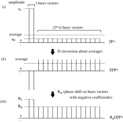
Figure 1: A variation of coefficients under the $(R_{\pi}D)$ transformation.

In this case, applying $D$ (we use the property of the inversion about average operation), and then, shifting the phase by $\pi$ on basis vectors which have negative coefficients, we can reduce a difference between new coefficients, $B_{0}$ and $B_{1}$, as shown in Figure 1. We write this phase shift operation by $R_{\pi}$. It can be expected that $[S-2^{n-2}(a_{min}+a_{min+1})]$ gets bigger by applying $(R_{\pi}D)$ successively. The next lemma shows it clearly.

Lemma 2: We consider a state,

$$|\Psi\rangle=[\underbrace{a_{0},\cdots,}_{\mbox{$2l$}}\underbrace{a_{1},\cdots,}_{\mbox{$2m$}}a_{2(l+m)},\cdots,a_{2^{n}-1}]\quad\quad\mbox{for $n\geq 4$},$$ (16)

where $0\leq a_{0}<a_{1}<a_{j}$ for $j=2(l+m),\cdots,2^{n}-1$. We assume that the number of elements $a_{0}$ is equal to $2l$ and the number of elements $a_{1}$ is equal to $2m$, where $l\geq 1$, $m\geq 1$, and $l+m\leq 2^{n-1}$. We also assume $S$, a sum of all coefficients of $|\Psi\rangle$, has the relation,

$$S-2^{n-2}(a_{0}+a_{1})<0.$$ (17)

Applying the inversion about average operation $D$ on $|\Psi\rangle$, and then, doing the phase shift transformation by $\pi$ on basis vectors which have negative coefficients, we obtain

$$R_{\pi}D|\Psi\rangle=[B_{0},\cdots,B_{1},\cdots,B_{2(l+m)},\cdots,B_{2^{n}-1}].$$ (18)

We define $\tilde{S}$ as a sum of all coefficients of $R_{\pi}D|\Psi\rangle$. We also define

$$\left\{\begin{array}[]{rcl}\epsilon^{(0)}&=&(2l-2^{n-1})a_{0}+(2^{n}-2l)a_{1},\\ \epsilon^{(1)}&=&(2l-2^{n-1})B_{0}+(2^{n}-2l)B_{1}.\end{array}\right.$$

1. We get $0<B_{0}<B_{1}<B_{j}$ for $j=2(l+m),\cdots,2^{n}-1$ and

   $$[\tilde{S}-2^{n-2}(B_{0}+B_{1})]-[S-2^{n-2}(a_{0}+a_{1})]>\epsilon^{(0)}>0.$$ (19)

2. We obtain the relation,

   $$\epsilon^{(1)}-\epsilon^{(0)}\geq\frac{2^{n}-2l}{2^{n-2}}[2^{n-2}(a_{0}+a_{1})-S]>0.$$ (20)

Proof: We can derive $D|\Psi\rangle=[a^{\prime}_{0},\cdots,a^{\prime}_{1},\cdots,a^{\prime}_{2(l+m)},\cdots,a^{\prime}_{2^{n}-1}]$, where

$$\left\{\begin{array}[]{rcl}2^{n-1}a^{\prime}_{0}&=&S-2^{n-1}a_{0},\\ 2^{n-1}a^{\prime}_{1}&=&S-2^{n-1}a_{1},\\ 2^{n-1}a^{\prime}_{j}&=&S-2^{n-1}a_{j},\quad\mbox{for $2(l+m)\leq j\leq 2^{n}-1$}.\end{array}\right.$$ (21)

It is clear that $S-2^{n-1}a_{0}>0$. Using the assumption of Eq. (17), we obtain $S-2^{n-1}a_{k}<0$ for $\forall k\neq 0$. Therefore, we get $R_{\pi}D|\Psi\rangle$ of Eq. (18), where

$$\left\{\begin{array}[]{rcl}2^{n-1}B_{0}&=&S-2^{n-1}a_{0},\\ 2^{n-1}B_{1}&=&-S+2^{n-1}a_{1},\\ 2^{n-1}B_{j}&=&-S+2^{n-1}a_{j},\quad\mbox{for $2(l+m)\leq j\leq 2^{n}-1$}.\end{array}\right.$$ (22)

We can derive a difference of $B_{1}$ and $B_{0}$ with the assumption of Eq. (17),

$$2^{n-1}(B_{1}-B_{0})=-2[S-2^{n-2}(a_{0}+a_{1})]>0.$$ (23)

It is clear that $B_{1}<B_{j}$ for $j=2(l+m),\cdots,2^{n}-1$. We obtain the relation, $0<B_{0}<B_{1}<B_{j}$ for $j=2(l+m),\cdots,2^{n}-1$.

Since

$$\tilde{S}=\frac{4l}{2^{n-1}}(S-2^{n-1}a_{0})-S,\quad\quad\mbox{and}\quad\quad B_{0}+B_{1}=a_{1}-a_{0},$$

we can derive $\Delta$ that is a variation of $[S-2^{n-2}(a_{0}+a_{1})]$ caused by the $(R_{\pi}D)$ operation,

$$\Delta = [\tilde{S}-2^{n-2}(B_{0}+B_{1})]-[S-2^{n-2}(a_{0}+a_{1})]$$ (24)

$$= 2(\frac{2l}{2^{n-1}}-1)S-(4l-2^{n-1})a_{0}.$$

To estimate $\Delta$ precisely, we prepare some useful relations. From the definition of $S$, we get

$$S=2la_{0}+2ma_{1}+\sum_{j=2(l+m)}^{2^{n}-1}a_{j}\geq 2la_{0}+(2^{n}-2l)a_{1}.$$ (25)

Using the assumption of Eq. (17) and Eq. (25), we can derive the relation,

$$0 > S-2^{n-2}(a_{0}+a_{1})$$ (26)

$$\geq 2la_{0}+(2^{n}-2l)a_{1}-2^{n-2}(a_{0}+a_{1})$$

$$= (2l-2^{n-2})a_{0}+(3\cdot 2^{n-2}-2l)a_{1}.$$

We modify the relation of Eq. (26) and get a rougher relation,

$$0>2la_{0}-2^{n-2}a_{1}+(3\cdot 2^{n-2}-2l)a_{1}=2la_{0}+(2^{n-1}-2l)a_{1}.$$ (27)

Because $0\leq a_{0}<a_{1}$, we obtain $2l-2^{n-1}>0$. Seeing this relation and Eq. (26) again, we also obtain

$$2l>3\cdot 2^{n-2}.$$ (28)

Here, we can estimate $\Delta$. Because of Eq. (28), we can substitute Eq. (25) for Eq. (24),

$$\Delta \geq 2(\frac{2l}{2^{n-1}}-1)[2la_{0}+(2^{n}-2l)a_{1}]-(4l-2^{n-1})a_{0}$$ (29)

$$= \frac{1}{2^{n-1}}(4l-3\cdot 2^{n-1})[(2l-2^{n-2})a_{0}+(3\cdot 2^{n-2}-2l)a_{1}]$$

$$\quad\quad\quad\quad\quad\quad+2^{n-2}(a_{1}-a_{0}).$$

Seeing Eq. (28), we find $3\cdot 2^{n-2}<2l<2^{n}$. Therefore, we can derive the relation, $0<(4l-3\cdot 2^{n-1})<2^{n-1}$. From Eq. (26) and Eq. (29), we can estimate $\Delta$,

$$\Delta>[(2l-2^{n-2})a_{0}+(3\cdot 2^{n-2}-2l)a_{1}]+2^{n-2}(a_{1}-a_{0})=\epsilon^{(0)}>0.$$ (30)

The first result is derived.

From the definition of Eq. (4) and Eq. (22), (25), (26), we can estimate the difference between $\epsilon^{(0)}$ and $\epsilon^{(1)}$,

$$\epsilon^{(1)}-\epsilon^{(0)} = \frac{1}{2^{n-1}}[(4l-3\cdot 2^{n-1})S-2^{n}a_{0}(2l-2^{n-1})]$$ (31)

$$\geq \frac{1}{2^{n-1}}\{(4l-3\cdot 2^{n-1})[2la_{0}+(2^{n}-2l)a_{1}]-(2l-2^{n-1})2^{n}a_{0}\}$$

$$= -\frac{2^{n}-2l}{2^{n-2}}[(3\cdot 2^{n-2}-2l)a_{1}+(2l-2^{n-2})a_{0}]$$

$$\geq \frac{2^{n}-2l}{2^{n-2}}[2^{n-2}(a_{0}+a_{1})-S]>0.$$

The second result is derived.  

Because of Lemma 2, doing the $(R_{\pi}D)$ transformations successively, we can make $[S-2^{n-2}(a_{0}+a_{1})]$ be nonnegative. We explain this matter as follows. We consider the state $|\Psi^{(0)}\rangle$ specified with coefficients, $0\leq a_{0}<a_{1}<a_{j}$ for $2(l+m)\leq j\leq 2^{n}-1$, and assume $S-2^{n-2}(a_{0}+a_{1})<0$. We apply $(R_{\pi}D)$ on $|\Psi^{(0)}\rangle$ and obtain $|\Psi^{(1)}\rangle$ described with coefficients, $0<B_{0}^{(1)}<B_{1}^{(1)}<B_{j}^{(1)}$ for $2(l+m)\leq j\leq 2^{n}-1$. Because of Lemma 2.1, we obtain

$$[S^{(1)}-2^{n-2}(B_{0}^{(1)}+B_{1}^{(1)})]-[S-2^{n-2}(a_{0}+a_{1})]>\epsilon^{(0)}>0,$$ (32)

where $S^{(1)}$ is a sum of all coefficients of $|\Psi^{(1)}\rangle$. Then, we assume $S^{(1)}-2^{n-2}(B_{0}^{(1)}+B_{1}^{(1)})<0$. After applying $(R_{\pi}D)$ on $|\Psi^{(1)}\rangle$, we get $|\Psi^{(2)}\rangle$ specified by $0<B_{0}^{(2)}<B_{1}^{(2)}<B_{j}^{(2)}$ for $2(l+m)\leq j\leq 2^{n}-1$. Because of Lemma 2.2, we get

$$[S^{(2)}-2^{n-2}(B_{0}^{(2)}+B_{1}^{(2)})]-[S^{(1)}-2^{n-2}(B_{0}^{(1)}+B_{1}^{(1)})]>\epsilon^{(1)}>\epsilon^{(0)}>0.$$ (33)

Consequently, if $S^{(k)}-2^{n-2}(B_{0}^{(k)}+B_{1}^{(k)})<0$, $[S^{(k+1)}-2^{n-2}(B_{0}^{(k+1)}+B_{1}^{(k+1)})]$ increases by $\epsilon^{(0)}(>0)$ at least. $k$ stands for the number of the $(R_{\pi}D)$ transformations applied on the state and $S^{(0)}=S$, $B_{0}^{(0)}=a_{0}$, $B_{1}^{(0)}=a_{1}$. Because $\epsilon^{(0)}$ is defined by $\{a_{0},a_{1}\}$ and $l$, $\epsilon^{(0)}$ is a definite finite value and positive. Repeating the $(R_{\pi}D)$ finite times, we can certainly make $[S^{(k)}-2^{n-2}(B_{0}^{(k)}+B_{1}^{(k)})]$ be nonnegative.

From Eq. (21) and Eq. (22), during the $(R_{\pi}D)$ iteration, we find that the phase shift is applied on the same basis vectors. Therefore, the $(R_{\pi}D)$ iteration can be understood as the inversion of Grover’s iteration. We use Grover’s iteration for enhancing an amplitude of a certain basis.

If $[S^{(k)}-2^{n-2}(B_{0}^{(k)}+B_{1}^{(k)})]$ comes to be nonnegative, we start to do the $(\tilde{R}DR)$ operation again. Using the $(\tilde{R}DR)$ operation and the $(R_{\pi}D)$ iteration, we can always transform $|\psi_{n}\rangle$ to the uniform superposition. How many times do we need to apply $(R_{\pi}D)$ on a state to obtain the relation, $S^{(k)}-2^{n-2}(B_{0}^{(k)}+B_{1}^{(k)})\geq 0$?

Estimating it, first, we introduce notations,

$$\epsilon^{(k)} = (2l-2^{n-1})B_{0}^{(k)}+(2^{n}-2l)B_{1}^{(k)},$$

$${\cal F}^{(k)} = S^{(k)}-2^{n-2}(B_{0}^{(k)}+B_{1}^{(k)}).$$ (34)

Because of Lemma 2, if ${\cal F}^{(k)}<0$, we get relations,

$${\cal F}^{(k+1)}-{\cal F}^{(k)} > \epsilon^{(k)}>0,$$

$$\epsilon^{(k+1)}-\epsilon^{(k)} \geq -[(2^{n}-2l)/2^{n-2}]{\cal F}^{(k)}\geq-{\cal F}^{(k)}/2^{n-3}>0,$$ (35)

where we give the minimum of $(2^{n}-2l)$ by $2$. Consequently, if ${\cal F}^{(0)}<{\cal F}^{(1)}<\cdots<{\cal F}^{(K-1)}<{\cal F}^{(K)}<0$, we estimate $\epsilon^{(k)}$ ($k=1,2,\cdots$) recurrently,

$$\epsilon^{(1)} \geq -x{\cal F}^{(0)}+\epsilon^{(0)}>-x{\cal F}^{(1)}(>0),$$

$$\epsilon^{(2)} \geq -x{\cal F}^{(1)}+\epsilon^{(1)}>-2x{\cal F}^{(1)}>-2x{\cal F}^{(2)}(>0),$$

$$\cdots$$

$$\epsilon^{(K)} \geq -x{\cal F}^{(K-1)}+\epsilon^{(K-1)}>-Kx{\cal F}^{(K-1)}>-Kx{\cal F}^{(K)}(>0),$$ (36)

where $x=1/2^{n-3}$. From these relations, assuming $Kx\leq 1$, we obtain

$$(0>){\cal F}^{(2)} > {\cal F}^{(1)}+\epsilon^{(1)}>(1-x){\cal F}^{(1)}>(1-x){\cal F}^{(0)},$$

$$(0>){\cal F}^{(3)} > {\cal F}^{(2)}+\epsilon^{(2)}>(1-2x){\cal F}^{(2)}>(1-x)(1-2x){\cal F}^{(0)},$$

$$\cdots$$

$${\cal F}^{(K+1)} > {\cal F}^{(K)}+\epsilon^{(K)}>(1-Kx){\cal F}^{(K)}\geq\prod_{k=1}^{K}(1-kx){\cal F}^{(0)}.$$ (37)

If ${\cal F}^{(K+1)}+\epsilon^{(0)}\geq 0$, we obtain ${\cal F}^{(K+2)}>0$ and we can conclude we need to apply the $(R_{\pi}D)$ transformation $(K+2)$ times at most. To derive the upper bound on times we have to apply the $(R_{\pi}D)$ transformations, we estimate $\epsilon^{(0)}$ and ${\cal F}^{(0)}$,

$$\epsilon^{(0)} \geq (2^{n}-2l)a_{1}\geq 2a_{1},$$

$${\cal F}^{(0)} > 2^{n}a_{0}-2^{n-2}(a_{0}+a_{1})\geq-2^{n-2}a_{1},$$ (38)

and we obtain

$${\cal F}^{(K+1)}+\epsilon^{(0)}\geq\prod_{k=1}^{K}(1-kx){\cal F}^{(0)}+\epsilon^{(0)}\geq-2^{n-2}a_{1}[\prod_{k=1}^{K}(1-kx)-x].$$ (39)

Therefore, to estimate the lower bound on $K$ for ${\cal F}^{(K+1)}+\epsilon^{(0)}\geq 0$, we have to derive the lower bound on $K$ for the large $n$ (small $x$) limit, where

$$\prod_{k=1}^{K}(1-kx)\leq x\quad\quad\mbox{for $0<x\ll 1$}.$$ (40)

Because $\lim_{m\to+\infty}[1-(1/m)]^{-m}=e(>2)$, if $x_{0}$ is small enough, we obtain

$$\prod_{k=\lceil\sqrt{1/x}\rceil}^{2\lceil\sqrt{1/x}\rceil-1}(1-kx)<(1-\frac{1}{\lceil\sqrt{1/x}\rceil})^{\lceil\sqrt{1/x}\rceil}<\frac{1}{2},$$ (41)

for $0<\forall x<x_{0}\ll 1$ ($\lceil\sqrt{1/x}\rceil$ is the minimum integer that does not below $\sqrt{1/x}$). Remembering $x=1/2^{n-3}$, we get

$$x>[\prod_{k=\lceil\sqrt{1/x}\rceil}^{2\lceil\sqrt{1/x}\rceil-1}(1-kx)]^{n-3}>\prod_{k=1}^{(n-2)\lceil\sqrt{1/x}\rceil-1}(1-kx).$$ (42)

Consequently, the lower bound on $K$ is $(n-2)\lceil\sqrt{1/x}\rceil-1\sim O(n2^{n/2})$. We have to apply the $(R_{\pi}D)$ transformation $O(n2^{n/2})$ times at most. (See §Appendix B.)

Using Eq. (22), we can compute $\{B_{k}\}$ with $poly(n)$ steps by classical computation, because the number of different coefficients in $\{B_{k}\}$ is equal to $(\lfloor n/2\rfloor+1)$.

5 The whole procedure

In this section, we show the whole procedure for building $|\psi_{n}\rangle$ and give a sketch of implementation for our procedure. We also show that we can use it for building more general entangled states.

As a result of discussion we have had, we obtain the whole procedure to build $|\psi_{n}\rangle$ as follows. (We describe the procedure reversely from $|\psi_{n}\rangle$ to the uniform superposition. Throughout our procedure, we take $\{|x\rangle|x\in\{0,1\}^{n}\}$ as basis vectors.)

1. We consider an $n$-qubit register that is in the state of $|\psi_{n}\rangle$ for an initial state. (We assume all coefficients of basis vectors are positive or equal to $0$.)

2. If the state of the register is equal to the uniform superposition, stop operations. If it is not equal to the uniform superposition, go to step 3.

3. Let $a_{min}$ be the minimum coefficient for basis vectors in the state of the register and $a_{min+1}$ be the coefficient next to $a_{min}$. Examine whether $a_{min}$ and $a_{min+1}$ satisfy the sufficient condition of Lemma 1 or not. If they satisfy it, carry out the $(\tilde{R}DR)$ operation, shift the phases of basis vectors which have negative coefficients by $\pi$, and then go to step 2. If they do not satisfy it, go to step 4.

4. Apply the $(R_{\pi}D)$ transformation on the register and go to step 3.

Before executing this procedure, we need to trace a variation of coefficients of basis in each step by classical computation, because we have to know which basis vectors have the coefficients $a_{min}$ and $a_{min+1}$, find the phase shift parameter of the $(\tilde{R}DR)$ operation, and so on. From these results, we construct a network of quantum gates. The amount of classical computation is comparable with the number of steps for the whole quantum transformations.

We now sketch out the points of networks of quantum gates for our procedure. Because it is a chain of phase shift transformations and Grover’s operation $D$s, we discuss the networks of quantum gates for them.

First, we discuss the phase shift transformation. In the $(\tilde{R}DR)$ operation, we shift the phases by $\theta$ on half of basis vectors which have coefficients $a_{k}$ (as $a_{min+1}$) and by $(-\theta)$ on the other half of them. Constructing networks for $R_{\theta}$, we prepare two registers and a unitary transformation $U_{f}$,

$$|x\rangle\otimes|y\rangle\stackrel{{\scriptstyle U_{f}}}{{\longrightarrow}}|x\rangle\otimes|y\oplus f(x)\rangle,$$ (43)

where the first (main) register is made from $n$ qubits, the second (auxiliary) register is made from $m=\lceil\log_{2}(n+1)\rceil$ qubits initialized to $|0\cdots 0\rangle$, and

$$f(x)=(\mbox{the number of ``$1$'' in the binary string of $x$}).$$ (44)

Obtaining $f(x)$ on classical computation, we need $O(nm)\sim O(n\log_{2}n)$ classical gates (XOR, and so on) and $O(m)\sim O(\log_{2}n)$ other auxiliary classical bits. Therefore, we can construct $U_{f}$ with $O(n\log_{2}n)$ elementary quantum gates ([1][14][15] and see §Appendix A).

To execute the selective phase shift efficiently, we apply it on the second register instead of the first register. Because the phase shift matrix defined in Eq. (3) is diagonal, we can do this way. After shifting the phases, we apply $U_{f}$ again and initialize the second register. Unnecessary entanglement between the first and the second register is removed.

To see these operations precisely, we apply $U_{f}$ on $|\psi_{n}\rangle$ defined in Eq. (2). We get

$$U_{f}|\psi_{n}\rangle\otimes|0\rangle = U_{f}\sum_{k=0}^{\lfloor n/2\rfloor}a_{k}|k\rangle_{s}\otimes|0\rangle$$ (47)

$$= \left\{\begin{array}[]{ll}\sum_{k=0}^{(n-1)/2}a_{k}[|k)\otimes|k\rangle+|n-k)\otimes|n-k\rangle],&\mbox{($n$ is odd)}\\ \sum_{k=0}^{(n/2)-1}a_{k}[|k)\otimes|k\rangle+|n-k)\otimes|n-k\rangle]\\ \quad\quad\quad\quad\quad\quad+a_{n/2}|n/2)\otimes|n/2\rangle,&\mbox{($n$ is even)}\end{array}\right.$$

where $|k)$ is an equally weighted superposition of $k$ excited qubits ($|k\rangle_{s}=|k)+|n-k)$ except for $|n/2\rangle_{s}=|n/2)$ where $n$ is even). We shift the phases of basis vectors $|k\rangle$, $|n-k\rangle$ on the second register, instead of $|k)$, $|n-k)$ (that contain $2(^{n}_{k})$ binary states) on the first register (where $k\neq n/2$). This implementation reduces the number of basis vectors on which we apply the phase shift operation from $2(^{n}_{k})$ to $2$, and we can save elementary quantum gates. Using another auxiliary qubit, we can carry out the phase shift with $O(\log_{2}n)$ elementary quantum gates ([14][16] and see §Appendix A). If $n$ is even and $k=n/2$, we can’t decide which basis vectors we have to shift the phases by $\theta$ or $(-\theta)$. In this case, we refer to not only $|n/2\rangle$ on the second register but also the first qubit of the first register (cf. $|\psi_{4}\rangle$ defined in Eq. (1)).

Then, we discuss how to construct the quantum network of $D$. It is known that $D$ can be decomposed to the form, $D=-WRW$, where $W=H^{(1)}\otimes\cdots\otimes H^{(n)}$ (the Walsh-Hadamard transformation on $n$ qubits of the main register), and $R$ is a phase shift by $\pi$ on $|0\cdots 0\rangle$ of $n$ qubits[6]. $D$ takes $O(n)$ steps.

We repeat the $(R_{\pi}D)$ transformation $O(n2^{n/2})$times at most before the $(\tilde{R}DR)$ operation. If we do the $(R_{\pi}D)$ iteration before every $(\tilde{R}DR)$, we carry out it $\lfloor n/2\rfloor$ times. Therefore, the $(R_{\pi}D)$ iterations take the main part of the whole steps. Because $(R_{\pi}D)$ takes $O(n\log_{2}n)$ steps, we need $O((n^{3}\log_{2}n)\times 2^{n/2})$ steps for the whole procedure in total at most.

Finally, we consider the case where all of $\{a_{k}\}$ are neither positive nor real. Doing the selective phase shift on the basis vectors with complex or negative real coefficients in $|\psi_{n}\rangle$ to cancel the phases, we obtain a superposition whose all coefficients are real and nonnegative. After this operation, we can apply our procedure on the state.

In our method, we don’t fully use the symmetry of $|\psi_{n}\rangle$. Essential points that we use are as follows. First, the number of basis vectors that have the same coefficient is always even. Second, we can efficiently shift the phase of half the basis vectors that have the same coefficients. Third, the number of different coefficients $\{a_{k}\}$ is $poly(n)$. Therefore, we can apply our method to build more general entangled states that have above properties.

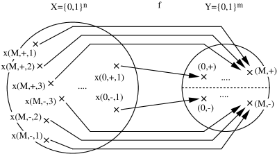
Figure 2: A function $f$ defined in Eq. (49).

Here, we discuss applying our method for building more general entangled states than $|\psi_{n}\rangle$. We consider an entangled state defined by a function $f$, as follows,

$$f:X=\{0,1\}^{n}\rightarrow Y=\{0,1\}^{m},$$ (48)

where $m=\lceil\log_{2}(M+1)\rceil+1$ and $M$ is polynomial in $n$. We assume we can label elements of image caused by $f$ from $X=\{0,1\}^{n}$ by $\{(0,\pm),(1,\pm),\cdots,(M,\pm)\}$. We also assume the number of $X$’s elements mapped to $(k,+)$ and the number of them mapped to $(k,-)$ are equal to $l_{k}$ for $k=0,\cdots,M$, where $2\sum_{k=0}^{M}l_{k}=2^{n}$. We can describe the function $f$ by

$$f(x(k,\epsilon,\zeta))=(k,\epsilon),$$ (49)

where $k=0,1,\cdots,M$, and $\epsilon=\pm$, and $\zeta=1,\cdots,l_{k}$, as shown in Figure 2.

Then we consider the following $n$-qubit partially entangled state,

$$|\Psi_{n}\rangle=\sum_{k=0}^{M}\sum_{\epsilon=\pm}\sum_{\zeta=1}^{l_{k}}c_{k}|x(k,\epsilon,\zeta)\rangle\quad\quad\mbox{for $n\geq 2$},$$ (50)

where $\{c_{k}\}$ are complex. The number of sets of basis vectors classified by $\{c_{k}\}$ is $(M+1)$, and the number of basis vectors that have the coefficient $c_{k}$ is $2l_{k}$.

Executing the selective phase shift efficiently, we apply $U_{f}$ of Eq. (49) to write $(k,\epsilon)$ on the $m$-qubit second register and apply phase shift transformation on it. We can shift the phase by $\theta$ or $(-\theta)$ according to $\epsilon$ in the $(\tilde{R}DR)$ operation. To transform $|\Psi_{n}\rangle$ to the uniform superposition, we have to do the $(\tilde{R}DR)$ operation $M$ times. Consequently, the $(R_{\pi}D)$ transformation is repeated $M\times O(n2^{n/2})$ times at most. It is desirable that $M$ is $poly(n)$.

6 Discussion

It is known that any unitary transformation $U$ $(\in\mbox{\boldmath$U$}(2^{n}))$ can be constructed from $O(n^{3}2^{2n})$ elementary gates at most[14]. In comparison with this most general case, our method is efficient, although the number of gates increases exponentially in $n$.

C. H. Bennett et al. discuss transmitting classical information via quantum noisy
channels[8]. It is shown when two transmissions of the two-Pauli channel are used, the optimal states for transmitting classical information are partially entangled states of two qubits. Therefore, we can expect our method is available for quantum communication.

Grover’s algorithm was proposed as a solution of the SAT(satisfiability) problems. It finds a certain combination from all of $2^{n}$ possible combinations of $n$ binary variables. From a different view, what Grover’s method does is enhancing an amplitude of a certain basis vector specified with an oracle for a superposition of $2^{n}$ basis vectors. In our method, we use Grover’s method for adjusting amplitudes of basis vectors.

We can’t show whether our procedure is optimal or not in view of the number of elementary gates. Because we don’t use the symmetry of $|\psi_{n}\rangle$ enough, our method seems to waste steps.

Recently, constructing approximately an optimal state for Ramsey spectroscopy by spin squeezing has been proposed[17]. This state also has symmetry like Eq. (2), and it is characterized by one parameter.

Acknowledgements

We would like to thank Dr. M. Okuda and Prof. A. Hosoya for critical reading and valuable comments.

Appendix A Networks of quantum gates

We construct networks of quantum gates for our method concretely. For notations of networks and quantum gates, we refer to A. Barenco et al.[14].

A.1 The network of $U_{f}$

$U_{f}$ (defined in Eq. (43), (44) or Eq. (49)) is given by the controlled gate, which causes the unitary transformation on the second register under the value of the first register. Constructing the controlled gate of $U_{f}$ with $poly(n)$ quantum elementary gates, we can use our method efficiently.

We consider a network for $U_{f}$ defined in Eq. (43) and Eq. (44). $f(x)$ represents the number of “$1$” bit in the binary string $x$. Writing the first (main) and second (auxiliary) register by $|X_{n},X_{n-1},\cdots,X_{2},X_{1}\rangle\otimes|S\rangle$, where $|S\rangle$ is made up of $m=\lceil\log_{2}(n+1)\rceil$ qubits and initialized to $|0\cdots 0\rangle$, we can write the quantum networks as the following program. (For the notation of the program, we referred to Cleve et al.[18].)

Program adder-1
	quantum registers:
	$X_{1},X_{2},\cdots,X_{n}$: qubit registers
	$S$: an m-qubit register
for $k=1$ to $n$ do
	$S\leftarrow(S+X_{k})\quad\mbox{mod}\;2^{m}$.

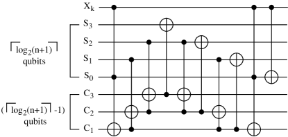
Figure 3: The network of the adder-2 for $m=\lceil\log_{2}(n+1)\rceil=4$.

To write a program for the addition of $X_{k}$ in the adder-1, we describe the qubits of the second register by $|S_{m-1},\cdots,S_{1},S_{0}\rangle$, introduce other auxiliary qubits $|C_{m-1},\cdots,C_{1}\rangle$, and use $C_{j}$ as a carry bit of addition at the $(j-1)$th bit. We can write the program as follows.

Program adder-2
	quantum registers:
	$X_{k}$: a qubit register
	$S_{0},S_{1},\cdots,S_{m-1}$: qubit registers
	$C_{1},C_{2},\cdots,C_{m-1}$: auxiliary qubit registers (initialized and finalized to 0)
$C_{1}\leftarrow C_{1}\oplus(S_{0}\land X_{k})$
for $j=2$ to $m-1$ do
		$C_{j}\leftarrow C_{j}\oplus(C_{j-1}\land S_{j-1})$
for $j=m-1$ down to $2$ do
		$S_{j}\leftarrow S_{j}\oplus C_{j}$
		$C_{j}\leftarrow C_{j}\oplus(C_{j-1}\land S_{j-1})$
$S_{1}\leftarrow S_{1}\oplus C_{1}$
$C_{1}\leftarrow C_{1}\oplus(S_{0}\land X_{k})$
$S_{0}\leftarrow S_{0}\oplus X_{k}$.

Because we don’t use interference, we can describe these operations with a higher level language of classical computation. In this program, to avoid obtaining unnecessary entanglement, we initialize and finalize all auxiliary qubits $\{|C_{j}\rangle\}$ to $|0\rangle$. Figure 3 shows a network of this program for $m=4$. Repeating the quantum network of the adder-2 for each $X_{k}$ $(k=1,\cdots,n)$, we can construct the adder-1.

We estimate the number of quantum elementary gates to construct the adder-1. In Figure 3, we use $2(\lceil\log_{2}(n+1)\rceil-1)$ Toffoli gates (that maps $|x,y,z\rangle\rightarrow|x,y,z\oplus(x\wedge y)\rangle$) and $\lceil\log_{2}(n+1)\rceil$ controlled-NOT gates for the adder-2. Because we repeat the adder-2 $n$ times, the number of the whole steps for the adder-1 is equal to $n(3\lceil\log_{2}(n+1)\rceil-2)$.

A.2 Construction of $\bigwedge_{n}(R_{z}(\alpha))$

From now on, we often use a $\bigwedge_{n}(R_{z}(\alpha))$ gate, where $R_{z}(\alpha)$ is given in the form,

$$R_{z}(\alpha)=\exp(i\alpha\sigma_{z}/2)=\left[\begin{array}[]{cc}\exp(i\alpha/2)&0\\ 0&\exp(-i\alpha/2)\end{array}\right].$$ (51)

(We describe the $\mbox{controlled}^{m}\mbox{-}U$ by $\bigwedge_{m}(U)$, where $\forall U\in\mbox{\boldmath$U$}(2)$. $\bigwedge_{m}(U)$ has an $m$-qubit control subsystem and a one-qubit target subsystem. It works as follows. If all $m$ qubits of control subsystem are equal to $|1\rangle$, $\bigwedge_{m}(U)$ applies $U$ on a target qubit. Otherwise $\bigwedge_{m}(U)$ does nothing. We can write the Toffoli gate by $\bigwedge_{2}(\sigma_{x})$, the controlled-NOT gate by $\bigwedge_{1}(\sigma_{x})$, and any $\mbox{\boldmath$U$}(2)$ gate for one qubit by $\bigwedge_{0}$.) Here, we consider how to construct it from elementary gates.

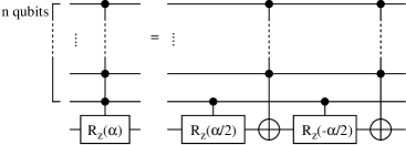
Figure 4: Decomposition of a $\bigwedge_{n}(R_{z}(\alpha))$ gate.

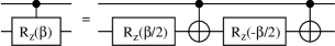
Figure 5: Decomposition of a $\bigwedge_{1}(R_{z}(\beta))$ gate.

At first, using relations,

$$R_{z}(\alpha/2)\sigma_{x}R_{z}(-\alpha/2)\sigma_{x}=R_{z}(\alpha),\quad\quad\mbox{and}\quad\quad R_{z}(\alpha/2)R_{z}(-\alpha/2)=\mbox{\boldmath$I$},$$

we can decompose a $\bigwedge_{n}(R_{z}(\alpha))$ gate to a $\bigwedge_{1}(R_{z}(\alpha/2))$ gate, a $\bigwedge_{1}(R_{z}(-\alpha/2))$ gate and two $\bigwedge_{n-1}(\sigma_{x})$ gates, as shown in Figure 4. Seeing Figure 5, we can decompose a $\bigwedge_{1}(R_{z}(\beta))$ gate to an $R_{z}(\beta/2)$ gate, an $R_{z}(-\beta/2)$ gate and two controlled-NOT gates. We have to only consider how to make a $\bigwedge_{n-1}(\sigma_{x})$ gate from elementary gates on an $(n+1)$-qubit network. Especially, we pay attention to the fact that there is a qubit which is not used by the $\bigwedge_{n-1}(\sigma_{x})$ gate on the network.

It is shown that, on an $(n+1)$-qubit network, where $n\geq 6$, a $\bigwedge_{n-1}(\sigma_{x})$ gate can be decomposed to $8(n-4)$ Toffoli gates[14]. Consequently, on the $(n+1)$-qubit network$(n\geq 6)$, a $\bigwedge_{n}(R_{z}(\alpha))$ gate can be decomposed to $16(n-4)$ Toffoli gates, four $\bigwedge_{1}(\sigma_{x})$ gates and four $\bigwedge_{0}$ gates. Therefore, $\bigwedge_{n}(R_{z}(\alpha))$ takes $8(2n-7)$ quantum elementary gates in total.

A.3 The phase shift on certain basis vectors

Figure 6 shows a quantum network for the selective phase shift by $\theta$ on a certain basis vector of the second register defined in Eq. (43). In Figure 6, we use a $\bigwedge_{m}(R_{z}(2\theta))$ gate. Setting the auxiliary qubit being $|0\rangle$, $\bigwedge_{m}(R_{z}(2\theta))$ generates an eigenvalue $\exp(i\theta)$ if and only if the second register is in the state $|1\cdots 1\rangle$. This technique is called “kick back”[16].

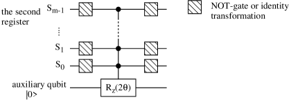
Figure 6: The network of the phase shift on the second register.

In Figure 6, a shaded box stands for the NOT-gate given by $\sigma_{x}$ ($|0\rangle\rightarrow|1\rangle$, $|1\rangle\rightarrow|0\rangle$) or the identity transformation. Deciding which gates are set in each shaded box, $\sigma_{x}$ or $I$, we can select a basis vector on which we shift the phase.

In case $m\geq 6$, it has been already shown that a $\bigwedge_{m}(R_{z}(2\theta))$ gate can be constructed from $8(2m-7)$ quantum elementary gates at most. Seeing Figure 6, we find that the selective phase shift on the second register takes $2m+8(2m-7)=2(9m-28)\sim O(m)$ gates at most. Building $|\psi_{n}\rangle$, we can carry out the phase shift on certain basis vectors on the second register with $O(\log_{2}n)$ steps.

A.4 The network of $D$

Figure 7 shows a network of $D$. Since this network consists of $4n$ $\bigwedge_{0}$ gates and a $\bigwedge_{n}(R_{z}(2\pi))$ gate, it takes $4(5n-14)$ elementary gates, in case $n\geq 6$. Therefore, $D$ takes $O(n)$ steps.

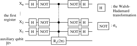
Figure 7: The network of $D$.

A.5 Estimation of steps

How many elementary gates do we need to construct $|\psi_{n}\rangle$ defined in Eq. (2) or $|\Psi_{n}\rangle$ defined in Eq. (50) from the uniform superposition? If $M$ (the number of sets of basis vectors classified by their coefficients) is $poly(n)$, and if the function $U_{f}$ defined in Eq. (43) can be constructed from $poly(n)$ elementary gates, the $(R_{\pi}D)$ iterations take the main part of the whole steps.

In the $(R_{\pi}D)$ transformation, we do the following operations. Applying $D$ on the $n$-qubit first register, preparing the initialized $m$-qubit second register, we apply $U_{f}$ on both of the registers as Eq. (43). Then, we shift the phases of basis vectors on the second register. Finally, we apply $U_{f}$ again to initialize the second register. It has been already shown $D$ takes $4(5n-14)$ steps, where $n\geq 6$. The number of steps that a network of $U_{f}$ takes depends on the function $f$. For instance, when we build $|\psi_{n}\rangle$, $U_{f}$ needs $O(n\log_{2}n)$ steps.

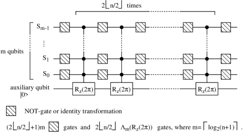
Figure 8: The network of the phase shift by $\pi$ on the second register for $R_{\pi}$

Figure 8 shows a network of the phase shift by $\pi$ on the second register with negative coefficients for $R_{\pi}$, in the case of building $|\psi_{n}\rangle$. To inverse signs of negative coefficients, we shift the phase at most for $\lfloor n/2\rfloor$ sets of basis vectors characterized by coefficients. Therefore, we shift the phases of $2\lfloor n/2\rfloor$ basis vectors of the second register at most. As a result, the network can be constructed from $(2\lfloor n/2\rfloor+1)\cdot\lceil\log_{2}(n+1)\rceil$ $\bigwedge_{0}$ gates and $2\lfloor n/2\rfloor$ $\bigwedge_{\lceil\log_{2}(n+1)\rceil}(R_{z}(2\pi))$ gates. We can carry out $R_{\pi}$ with $O(n\log_{2}n)$ steps. Similarly, in the case of $|\Psi_{n}\rangle$, we can estimate $R_{\pi}$ takes $O(M\log_{2}M)$ steps.

Building $|\psi_{n}\rangle$, we repeat the $(R_{\pi}D)$ transformation $O(n2^{n/2})$times at most before the $(\tilde{R}DR)$ operation. If we do the $(R_{\pi}D)$ iteration before every $(\tilde{R}DR)$, we carry out it $\lfloor n/2\rfloor$ times. Consequently, we need $O((n^{3}\log_{2}n)\times 2^{n/2})$ steps for the whole procedure in total at most.

Appendix B A variation of coefficients during the $(R_{\pi}D)$ iteration

We explicitly derive a variation of coefficients during the $(R_{\pi}D)$ iteration for the case described in (15), and estimate how many times do we need to apply $(R_{\pi}D)$ to make $[S^{(k)}-2^{n-2}(B_{0}^{(k)}+B_{1}^{(k)})]$ be nonnegative. We find it takes $O(2^{n/2})$ times, in spite of the results, $O(n2^{n/2})$ times, in §4.

Applying $(R_{\pi}D)$ on $|\Psi\rangle$ defined by (15), we obtain $R_{\pi}D|\Psi\rangle=[B_{0}^{(1)},\cdots,B_{1}^{(1)},\cdots]$, where

$$\left\{\begin{array}[]{lll}2^{n-1}B_{0}^{(1)}&=S-2^{n-1}a_{0}&=(2^{n-1}-t)a_{0}+ta_{1},\\ 2^{n-1}B_{1}^{(1)}&=-S+2^{n-1}a_{1}&=-(2^{n}-t)a_{0}+(2^{n-1}-t)a_{1}.\end{array}\right.$$ (52)

Referring to [7], we write $t$ as

$$\sin^{2}\theta=\frac{t}{2^{n}},\quad(\cos^{2}\theta=\frac{2^{n}-t}{2^{n}}),$$ (53)

where $0<\theta<(\pi/2)$, and write $\{a_{0},a_{1}\}$ as

$$a_{0}=\frac{\sin\alpha}{\sqrt{2^{n}-t}},\quad a_{1}=\frac{\cos\alpha}{\sqrt{t}},$$ (54)

where $0\leq\alpha<(\pi/2)$. Using (52), (53), and (54), we can describe $\{B_{0}^{(1)},B_{1}^{(1)}\}$ by

$$\left\{\begin{array}[]{lll}B_{0}^{(1)}&=(1/\sqrt{2^{n}})[\cos 2\theta(\sin\alpha/\cos\theta)+2\sin\theta\cos\alpha]&=\sin(\alpha+2\theta)/\sqrt{2^{n}-t},\\ B_{1}^{(1)}&=(1/\sqrt{2^{n}})[-2\cos\theta\sin\alpha+\cos 2\theta(\cos\alpha/\sin\theta)]&=\cos(\alpha+2\theta)/\sqrt{t}.\end{array}\right.$$ (55)

Writing coefficients of the state on which $(R_{\pi}D)$ has been applied $k$ times as $B_{0}^{(k)}$ and $B_{1}^{(k)}$, we obtain

$$B_{0}^{(k)}=\frac{\sin(\alpha+2k\theta)}{\sqrt{2^{n}-t}},\quad\quad B_{1}^{(k)}=\frac{\cos(\alpha+2k\theta)}{\sqrt{t}}\quad\quad\mbox{for $k=0,1,2,\cdots,$}$$ (56)

where $B_{0}^{(0)}=a_{0}$, $B_{1}^{(0)}=a_{1}$.

Defining $S^{(k)}=(2^{n}-t)B_{0}^{(k)}+tB_{1}^{(k)}$, we can derive

$$S^{(k)}-2^{n-2}(B_{0}^{(k)}+B_{1}^{(k)})$$ (57)

$$= (3\cdot 2^{n-2}-t)B_{0}^{(k)}+(t-2^{n-2})B_{1}^{(k)}$$

$$= \sqrt{2^{n}}\{\sin[\alpha+(2k+1)\theta]-\frac{1}{2\sin 2\theta}\cos[\alpha+(2k-1)\theta]\}$$

$$= -\frac{\sqrt{2^{n-2}}}{\sin 2\theta}F^{(k)},$$

where

$$F^{(k)}=\cos[\alpha+(2k+3)\theta].$$ (58)

Since $0<\theta<(\pi/2)$ and $\sin 2\theta>0$, it depends on a sign of $F^{(k)}$ whether $[S^{(k)}-2^{n-2}(B_{0}^{(k)}+B_{1}^{(k)})]$ is negative or not. (With some calculations, we can confirm that (56) and (57) satisfy Lemma 2.)

Because of $0\leq\alpha<(\pi/2)$, if $(2k+3)\theta=(\pi/2)$, it is always accomplished that $F^{(k)}\leq 0$ and $S^{(k)}-2^{n-2}(B_{0}^{(k)}+B_{1}^{(k)})\geq 0$. Therefore, the number of times we need to apply $(R_{\pi}D)$ doesn’t exceed $k_{MAX}$, which is given as

$$k_{MAX}=\frac{1}{2\theta}(\frac{\pi}{2}-3\theta).$$ (59)

On the other hand, we can write $\theta$ as $\sin\theta=\sqrt{t/2^{n}}$ from (53), and the minimum value of $t$ is $2$. Taking the limit that $t\sim O(1)$ and $n$ is large enough, we obtain a relation, $\sin\theta\sim\theta\sim\sqrt{t/2^{n}}$ and

$$k_{MAX}\sim\frac{\pi}{4}\sqrt{\frac{2^{n}}{t}}\sim O(2^{n/2}).$$ (60)

The $(R_{\pi}D)$ transformation is repeated $O(2^{n/2})$ times at most to make $[S^{(k)}-2^{n-2}(B_{0}^{(k)}+B_{1}^{(k)})]$ be nonnegative.

References

- [1] R. P. Feynman, Feynman Lectures on Computation (Addison-Wesley, 1996).
- [2] D. Deutsch and R. Jozsa, Proc. R. Soc. Lond. A 439, 553 (1992).
- [3] D. Simon, “On the power of quantum computation” in Proc. 35th Ann. Symp. on the Foundations of Computer Science (IEEE Computer Society, Los Alamitos, 1994), pp. 116-123.
- [4] P. W. Shor, “Algorithms for Quantum Computation: Discrete Logarithms and Factoring” in Proc. 35th Ann. Symp. on the Foundations of Computer Science (IEEE Computer Society, Los Alamitos, 1994), pp. 124-134. An expanded version is P. W. Shor, SIAM J. Comput. 26, 1484 (1997).
- [5] A. Ekert and R. Jozsa, Rev. Mod. Phys. 68, 733 (1996).
- [6] L. K. Grover, “A fast quantum mechanical algorithm for database search” in Proc. 28th Ann. ACM Symp. on the Theory of Computing (STOC), 1996, pp. 212-219.
- [7] M. Boyer, G. Brassard, P. Høyer and A. Tapp, “Tight bounds on quantum searching”, LANL e-print quant-ph/9605034 (1996), published in M. Boyer et al. Fortschr. Phys. 46 (1998) 4-5, 493-505.
- [8] C. H. Bennett, C. A. Fuchs and J. A. Smolin, “Entanglement-Enhanced Classical Communication on a Noisy Quantum Channel” in Quantum Communication, Computing, and Measurement, ed. Hirota et al. (Plenum Press, New York, 1997), pp. 79-88.
- [9] D. J. Wineland, J. J. Bollinger, W. M. Itano, F. L. Moore and D. J. Heinzen, Phys. Rev. A 46, R6797 (1992).
- [10] D. J. Wineland, J. J. Bollinger, W. M. Itano and D. J. Heinzen, Phys. Rev. A 50, 67 (1994).
- [11] M. Kitagawa and M. Ueda, Phys. Rev. Lett. 67, 1852 (1991).
- [12] C. H. Bennett, D. P. DiVincenzo, J. A. Smolin and W. K. Wootters, Phys. Rev. A 54, 3824 (1996).
- [13] S. F. Huelga, C. Macchiavello, T. Pellizzari, A. K. Ekert, M. B. Plenio and J. I. Cirac, Phys. Rev. Lett. 79, 3865 (1997).
- [14] A. Barenco, C. H. Bennett, R. Cleve, D. P. DiVincenzo, N. Margolus, P. Shor, T. Sleator, J. Smolin and H. Weinfurter, Phys. Rev. A 52, 3457 (1995).
- [15] C. H. Bennett, IBM J. Res. Develop. 17, 525 (1973).
- [16] R. Cleve, A. Ekert, C. Macchiavello and M. Mosca, Proc. R. Soc. Lond. A 454, 339 (1998).
- [17] D. Ulam-Orgikh and M. Kitagawa, “Spin Squeezing as a Quantum Algorithm for Optimal Entanglement”, QIT99-22, Osaka Univ., November 1999.
- [18] R. Cleve and D. P. DiVincenzo, Phys. Rev. A 54, 2636 (1996).