[

Violation of Bell’s inequality under strict Einstein locality conditions

Abstract

We observe strong violation of Bell’s inequality in an Einstein, Podolsky and Rosen type experiment with independent observers. Our experiment definitely implements the ideas behind the well known work by Aspect et al. We for the first time fully enforce the condition of locality, a central assumption in the derivation of Bell’s theorem. The necessary space-like separation of the observations is achieved by sufficient physical distance between the measurement stations, by ultra-fast and random setting of the analyzers, and by completely independent data registration.

]

The stronger-than-classical correlations between entangled quantum systems, as first discovered by Einstein, Podolsky and Rosen (EPR) in 1935[1], have ever since occupied a central position in the discussions of the foundations of quantum mechanics. After Bell’s discovery[2] that EPR’s implication to explain the correlations using hidden parameters would contradict the predictions of quantum physics, a number of experimental tests have been performed[3, 4, 5]. All recent experiments confirm the predictions of quantum mechanics. Yet, from a strictly logical point of view, they don’t succeed in ruling out a local realistic explanation completely, because of two essential loopholes. The first loophole builds on the fact that all experiments so far detect only a small subset of all pairs created[6]. It is therefore necessary to assume that the pairs registered are a fair sample of all pairs emitted. In principle this could be wrong and once the apparatus is sufficiently refined the experimental observations will contradict quantum mechanics. Yet we agree with John Bell that

”…it is hard for me to believe that quantum mechanics works so nicely for inefficient practical set-ups and is yet going to fail badly when sufficient refinements are made. Of more importance, in my opinion, is the complete absence of the vital time factor in existing experiments. The analyzers are not rotated during the flight of the particles.”[7]

This is the second loophole which so far has only been encountered in an experiment by Aspect et al.[4] where the directions of polarization analysis were switched after the photons left the source. Aspect et al., however, used periodic sinusoidal switching, which is predictable into the future. Thus communication slower than the speed of light, or even at the speed of light [8] could in principle explain the results obtained. Therefore this second loophole is still open.

The assumption of locality in the derivation of Bell’s theorem requires that the measurement processes of the two observers are space-like separated (Fig. 1). This means that it is necessary to freely choose a direction for analysis, to set the analyzer and finally to register the particle such that it is impossible for any information about these processes to travel via any (possibly unknown) channel to the other observer before he, in turn, finishes his measurement[9]. Selection of an analyzer direction has to be completely unpredictable which necessitates a physical random number generator. A numerical pseudo-random number generator can not be used, since its state at any time is predetermined. Furthermore, to achieve complete independence of both observers, one should avoid any common context as would be conventional registration of coincidences as in all previous experiments[10]. Rather the individual events should be registered on both sides completely independently and compared only after the measurements are finished. This requires independent and highly accurate time bases on both sides.

In our experiment for the first time any mutual influence between the two observations is excluded within the realm of Einstein locality. To achieve this condition the observers “Alice” and “Bob” were spatially separated by 400 m across the Innsbruck university science campus. We used polarization entangled photon pairs which were sent to the observers through optical fibers[11]. About 250 m of each 500 m long cable was laid out and the rest was left coiled at the source. This, we remark, has no influence on the timing argument because the optical elements of the source and the locally coiled fibers can be seen as jointly forming the effective source of the experiment (Fig. 1). The difference in fiber length was less than 1 m which means that the photons were registered simultaneously within 5 ns.

As stated above, we define an individual measurement to last from the first point in time which can influence the choice of the analyzer setting until the final registration of the photon. In order to rule out subluminal as well as luminal communication between observers these individual measurements had to be shorter than $1.3{\rm\mu s}$, the time for direct communication at the speed of light. This we achieved using high speed physical random number generators and fast electro-optic modulators. Independent data registration was performed by each observer having his own time interval analyzer and atomic clock, synchronized only once before each experiment cycle.

Our source of polarization entangled photon pairs is degenerate type-II parametric down-conversion[5] where we pump a BBO-crystal with 400 mW of 351 nm light from an Argon-ion-laser. A telescope was used to narrow the UV-pump beam[12], in order to enhance the coupling of the 702 nm photons into the two single-mode glass fibers. On the way to the fibers, the photons passed a half-wave plate and the compensator crystals necessary to compensate for in-crystal birefringence and to adjust the internal phase $\varphi$ of the entangled state $|\Psi\rangle=1/\sqrt{2}(|H\rangle_{1}|V\rangle_{2}+{\rm e}^{i\varphi}|V\rangle_{1}|H\rangle_{2})$, which we chose $\varphi=\pi$.

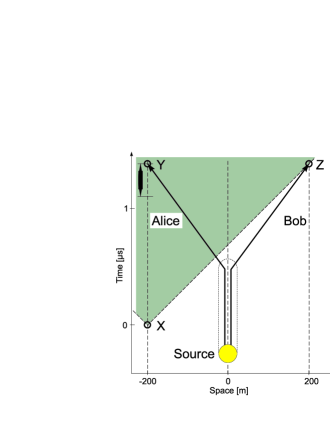
FIG. 1.: Spacetime diagram of our Bell experiment. Selecting a random analyzer direction, setting the analyzer and finally detecting a photon constitute the measurement process. This process on Alice’s side must fully lie inside the shaded region which is, during Bob’s own measurement, invisible to him as a matter of principle. For our setup this means that the decision about the setting has to be made after point “X” if the corresponding photons are detected at spacetime points “Y” and “Z” respectively. In our experiment the measurement process (indicated by a short black bar) including the choice of a random number only took less than a tenth of the maximum allowed time. The vertical parts of the kinked photon world lines emerging from the source represent the fiber coils at the source location.

The single-mode optical fibers had been selected for a cutoff wavelength close to 700 nm to minimize coupling losses. Manual fiber polarization controllers were inserted at the source location into both arms to be able to compensate for any unitary polarization transformation in the fiber cable. Depolarization within the fibers was found to be less than 1% and polarization proved to be stable (rotation less than $1^{\circ}$) within an hour.

Each of the observers switched the direction of local polarization analysis with a transverse electro-optic modulator. It’s optic axes was set at $45^{\circ}$ with respect to the subsequent polarizer. Applying a voltage causes a rotation of the polarization of light passing through the modulator by a certain angle proportional to the voltage[13]. For the measurements the modulators were switched fast between a rotation of $0^{\circ}$ and $45^{\circ}$.

The modulation systems (high-voltage amplifier and electro-optic modulator) had a frequency range from DC to 30 MHz. Operating the systems at high frequencies we observed a reduced polarization contrast of 97% (Bob) and 98% (Alice). This, however, is no real depolarization but merely reflects the fact that we are averaging over the polarization rotation induced by an electrical signal from the high-voltage amplifier, which is not of perfectly rectangular shape.

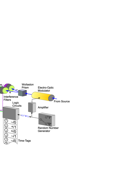
FIG. 2.: One of the two observer stations. A random number generator is driving the electro-optic modulator. Silicon avalanche photodiodes are used as detectors. A “time tag” is stored for each detected photon together with the corresponding random number “0” or “1” and the code for the detector “$+$” or “$-$” corresponding to the two outputs of the Wollaston prism polarizer. All alignments and adjustments were pure local operations that did not rely on a common source or on communication between the observers.

The actual orientation for local polarization analysis was determined independently by a physical random number generator. This generator has a light-emitting diode (coherence time $t_{c}\approx$10 fs) illuminating a beam-splitter whose outputs are monitored by photomultipliers. The subsequent electronic circuit sets its output to “0”(“1”) upon receiving a pulse from photomultiplier “0”(“1”). Events where both photomultipliers register a photon within $\triangle t\leq$ 2 ns are ignored. The resulting binary random number generator has a maximum toggle frequency of 500 MHz. By changing the source intensity the mean interval was adjusted to about 10 ns in order to have a high primary random bit rate[14, 15]. Certainly this kind of random-number generator is not necessarily evenly distributed. For a test of Bell’s inequality it is, however, not necessary to have perfectly even distribution, because all correlation functions are normalized to the total number of events for a certain combination of the analyzers’ settings. Still, we kept the distribution even to within 2% in order to obtain an approximately equal number of samples for each setting. The distribution was adjusted by equalizing the number of counts of the two photomultipliers through changing their internal photoelectron amplification. Due to the limited speed of the subsequent modulation system it was sufficient to sample this random number generator periodically at a rate of 10 MHz.

The total of the delays occurring in the electronics and optics of our random number generator, sampling circuit, amplifier, electro-optic modulator and avalanche photodiodes was measured to be 75 ns. Allowing for another 25 ns, to be sure that the autocorrelation of the random number generator output signal is sufficiently low, it was safe to assume that the specific choice of an analyzer setting would not be influenced by any event more than 100 ns earlier. This was much shorter than the $1.3\mu$s that any information about the other observer’s measurement would have been retarded.

The photons were detected by silicon avalanche photodiodes with dark count rates (noise) of a few hundred per second. This is very small compared to the 10.000 – 15.000 signal counts per second per detector. The pulses of each detector were fed into constant fraction discriminators to achieve accurate timing, and from there into the logic circuits. These logic circuits were responsible for disregarding events that occurred during transitions of the switch signal and generating an extra signal indicating the position of the switch. Finally all signals were time-tagged in special time interval analyzers, which allowed us to record the events with 75 ps resolution and 0.5 ns accuracy referenced to a rubidium standard together with the appendant switch position. The overall dead time of an individual detection channel was approximately $1{\mu}s$.

Using an auxiliary input of our time interval analyzers we synchronized Alice’s and Bob’s time scales by sending laser pulses (670 nm wavelength, 3 ns width) through a second optical fiber from the center to the observing stations. While the actual jitter between these pulses was measured in the laboratory to be less than 0.5 ns, the auxiliary input of the time interval analyzers had a resolution not better than 20 ns thus limiting synchronization accuracy. This non-perfect synchronization only limited our ability to exactly predict the apparent time shift between Alice’s and Bob’s data series, but did not in any way degrade time resolution or accuracy. It is important, however, that this uncertainty was smaller than the dead time of our detectors, because otherwise data analysis would have been much more complex.

Each observer station featured a PC which stored the tables of time tags accumulated in an individual measurement. Long after measurements were finished we analyzed the files for coincidences with a third computer. Coincidences were identified by calculating time differences between Alice’s and Bob’s time tags and comparing these with a time window (typically a few ns). As there were four channels on each side — two detectors with two switch positions — this procedure yielded 16 coincidence rates, appropriate for the analysis of Bell’s inequality. The coincidence peak was nearly noise-free (${\rm SNR}>100$) with approximately Gaussian shape and a width (FWHM) of about 2 ns. All data reported here were calculated with a window of 6 ns.

There are many variants of Bell’s inequalities. Here we use a version first derived by Clauser et al.[16] (CHSH) since it applies directly to our experimental configuration. The number of coincidences between Alice’s detector $i$ and Bob’s detector $j$ is denoted by $C_{ij}(\alpha,\beta)$ with $i,j\in\{\rm{+,-}\}$ where $\alpha$ and $\beta$ are the directions of the two polarization analyzers and “$+$” and “$-$” denote the two outputs of a two-channel polarizer respectively. If we assume that the detected pairs are a fair sample of all pairs emitted, then the normalized expectation value $E(\alpha,\beta)$ of the correlation between Alice’s and Bob’s local results is $E(\alpha,\beta)=[C_{++}(\alpha,\beta)+C_{--}(\alpha,\beta)-C_{+-}(\alpha,\beta)-C_{-+}(\alpha,\beta)]/N$, where $N$ is the sum of all coincidence rates. In a rather general form the CHSH inequality reads

$$S(\alpha,\alpha^{\prime},\beta,\beta^{\prime}) = |E(\alpha,\beta)-E(\alpha^{\prime},\beta)|+$$ (2)

$$+|E(\alpha,\beta^{\prime})+E(\alpha^{\prime},\beta^{\prime})|\leq 2.$$

Quantum theory predicts a sinusoidal dependence for the coincidence rate $C^{qm}_{++}(\alpha,\beta)\propto\sin^{2}(\beta-\alpha)$ on the difference angle of the analyzer directions in Alice’s and Bob’s experiments. The same behavior can also be seen in the correlation function $E^{qm}(\alpha,\beta)=-\cos(2(\beta-\alpha))$. Thus, for various combinations of analyzer directions $\alpha,\beta,\alpha^{\prime},\beta^{\prime}$ these functions violate Bell’s inequality. Maximum violation is obtained using the following set of angles $S^{qm}_{\rm max}=S^{qm}(0^{\circ},45^{\circ},22.5^{\circ},67.5^{\circ})=2\sqrt{2}=2.82>2$

If, however, the perfect correlations ($\alpha-\beta=0^{\circ}$ or $90^{\circ}$) have a reduced visibility $V\leq 1$ then the quantum theoretical predictions for $E$ and $S$ are reduced as well by the same factor independent of the angle. Thus, because the visibility of the perfect correlations in our experiment was about 97% we expect $S$ to be not higher than 2.74 if alignment of all angles is perfect and all detectors are equally efficient.

We performed various measurements with the described setup. The data presented in Fig. 3 are the result of a scan of the DC bias voltage in Alice’s modulation system over a 200 V range in 5 V steps. At each point a synchronization pulse triggered a measurement period of 5 s on each side. From the time-tag series we extracted coincidences after all measurements had been finished. Fig. 3 shows four of the 16 resulting coincidence rates as functions of the bias voltage. Each curve corresponds to a certain detector and a certain modulator state on each side. A nonlinear $\chi^{2}$-fit showed perfect agreement with the sine curve predicted by quantum theory. Visibility was 97% as one could have expected from the previously measured polarization contrast. No oscillations in the singles count rates were found. We want to stress again that the accidental coincidences have not been subtracted from the plotted data.

In order to give quantitative results for the violation of Bell’s inequality with better statistics, we performed experimental runs with the settings $0^{\circ},45^{\circ}$ for Alice’s and $22.5^{\circ},67.5^{\circ}$ for Bob’s polarization analyzer. A typical observed value of the function $S$ in such a measurement was $S=2.73\pm 0.02$ for 14700 coincidence events collected in 10 s. This corresponds to a violation of the CHSH inequality of 30 standard deviations assuming only statistical errors. If we allow for asymmetries between the detectors and minor errors of the modulator voltages our result agrees very well with the quantum theoretical prediction.

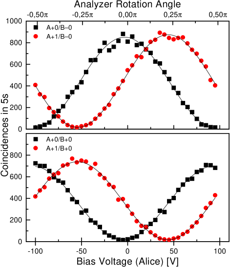
FIG. 3.: Four out of sixteen coincidence rates between various detection channels as functions of bias voltage (analyzer rotation angle) on Alice’s modulator. A$+$1/B$-$0 for example are the coincidences between Alice’s “$+$” detector with switch having been in position “1” and Bob’s “$-$” detector with switch position “0”. The difference in height is explained by different efficiencies of the detectors.

While our results confirm the quantum theoretical predictions[17], we admit that, however unlikely, local realistic or semi-classical interpretations are still possible. Contrary to all other statistical observations we would then have to assume that the sample of pairs registered is not a faithful representative of the whole ensemble emitted. While we share Bell’s judgement about the likelihood of that explanation[7], we agree that an ultimate experiment should also have higher detection/collection efficiency, which was 5% in our experiment.

Further improvements, e.g. having a human observers choose the analyzer directions would again necessitate major improvements of technology as was the case in order to finally, after more than 15 years, go significantly beyond the beautiful 1982 experiment of Aspect et al[4]. Expecting that any improved experiment will also agree with quantum theory, a shift of our classical philosophical positions seems necessary. Among the possible implications are nonlocality or complete determinism or the abandonment of counterfactual conclusions. Whether or not this will finally answer the eternal question: “Is the moon there, when nobody looks?”[18], is certainly up to the reader’s personal judgement.

This work was supported by the Austrian Science Foundation (FWF), project S6502, by the US NSF grant no. PHY 97-22614, and by the APART program of the Austrian Academy of Sciences.

REFERENCES

- [1] A. Einstein, B. Podolsky, and N. Rosen, Phys. Rev. 47, 777 (1935).
- [2] J. S. Bell, Physics 1, 195 (1965).
- [3] S. J. Freedman, J. F. Clauser, Phys. Rev. Lett. 28 938 (1972).
- [4] A. Aspect, J. Dalibard, and G. Roger, Phys. Rev. Lett. 49, 1804 (1982).
- [5] P.G. Kwiat, K. Mattle, H. Weinfurter, A. Zeilinger, A. V. Sergienko, and Y. Shih, Phys. Rev. Lett. 75, 4337 (1995).
- [6] P. Pearle, Phys Rev. D 2, 1418 (1970).
- [7] The observation that the photons in a pair, as used by us, are always found to have different polarization can not as easily be understood as the fact that the socks in a pair, as worn by Bertlmann, are always found to have different color. J.S. Bell, “Bertlmann’s socks and the nature of reality”, J. de Physique, C2, (suppl. au n. 3) 41 (1981) reprinted in Speakable and Unspeakable in Quantum Mechanics, pp. 139-158, Cambridge University Press, Cambridge 1987.
- [8] A. Zeilinger, Phys. Lett. A 118, 1 (1986).
- [9] G. Weihs, H. Weinfurter, and A. Zeilinger in: Experimental Metaphysics, pp. 271-280, R. S. Cohen et al. Eds., Kluwer Academic Publishers, Dordrecht 1997; G. Weihs, H. Weinfurter, and A. Zeilinger, Acta Physica Slovaca 47 337 (1997).
- [10] P. V. Christiansen, Physics Today 38, 11 (November 1985).
- [11] W. Tittel, J. Brendel, B. Gisin, T. Herzog, H. Zbinden, N. Gisin, Phys. Rev. A 57, 3229 (1998).
- [12] P. R. Tapster, J. G. Rarity, and P. C. M. Owens, Phys. Rev. Lett. 73, 1923 (1994); C. H. Monken, P. H. Souto Ribeiro, and S. Pádua, Phys. Rev. A 57, R2267 (1998).
- [13] Precisely speaking, the modulator introduces a phase shift between the linearly polarized components parallel and perpendicular to its optic axis (at ). Together with two quarter-wave plates (at or ) before and after the modulator this results in a polarization rotation in real space as usually seen in circularly birefringent media. The latter quarter-wave plate can be abandoned here because it is parallel to the axis of the subsequent polarizer and thus introduces only a phase which cannot be measured anyway. The quarter-wave plate in front of the modulator is substituted by our fiber and the initial polarization controllers.
- [14] U. Achleitner, master thesis, University of Innsbruck, Innsbruck 1997.
- [15] We tested our random-number-generator for exponential distribution of the occurring time intervals, for maximum entropy, and for short autocorrelation. Further we applied many special tests normally used to judge the quality of pseudo-random-number-generators [19]. These results will be the subject of a future publication.
- [16] J. F. Clauser, M. A. Horne, A. Shimony, and R. A. Holt, Phys. Rev. Lett. 23, 880 (1969).
- [17] Original sets of data are available at our web-site “http://www.quantum.at”. We would appreciate receiving suggestions for possible variations of the experiment.
- [18] N. D. Mermin, Physics Today 38, 38 (April 1985).
- [19] G.Marsaglia, Computers & Mathematics with Applications 9, 1 (1993); “The Marsaglia Random Number CDROM including the Diehard Battery of Tests of Randomness” is available from Prof. George Marsaglia, Florida State University.