Abstract

We explain the meaning of dynamical manipulation, and we illustrate its mechanism by using a system composed of a charged particle in a Penning trap. It is shown that by means of appropriate electric shocks (delta-like pulses) applied to the trap walls one can induce the squeezing transformation. The geometric phases associated to some cyclic evolutions, induced either by the standard fields of the Penning trap or by the superposition of these plus a rotating magnetic field, are analysed.

1 Introduction

The quantum control, or wavepacket engeenering, is one of suggestive subjects in Quantum Mechanics (QM). The very name reflects the dreams of almost any physicist: to be able to induce a physical system to make anything we wish [1]-[13]. Since long time ago we have been involved with that subject using a specific name: dynamical manipulation problem. My goals in this work are diverse:

• To explain what we mean precisely by dynamical manipulation

• To illustrate how it works in a realistic physical arrangement, namely the Penning trap

• To show the relation between dynamical manipulation and some ‘hot’ subjects in QM as squeezing and geometric phases

Having this in mind, this work has been organized as follows. In section 2 some generalities of the manipulation problem will be presented. Some specific dynamical processes, the evolution loops, will be introduced, and we will explain that they can be used in order to generate an arbitrary unitary transformation. In particular, they will be useful to induce the free evolution going back in time. In section 3 those general techniques will be applied to a realistic arrangement, namely, the Penning trap. Thus, it will be shown that the evolution loops occur in the Penning trap, and they will be called Penning loops. The ‘perturbed’ Penning loops will be used as a starting point to induce the squeezing transformation (in general the scale operation) and the Fourier-like transformation. In section 4 the general setting of the geometric (Aharonov-Anandan) phase will be shortly presented. Section 5 will stablish the connection between the geometric phase and the Penning loops (perturbed and unperturbed). The paper will end with some general conclusions.

2 Manipulation problem

Motivation: at first sight there is an asymmetry in nature so that the evolution forward in time is privileged. One might think that certain unitary operators cannot be dynamically achieved, e.g., the inverted free evolution towards the past (backwards in time)

$$e^{i\lambda{p^{2}\over 2}},\qquad\lambda>0.$$

The dynamical manipulation problem tries precisely to answer the question: can any given unitary transformation $U$ on a physical system be dynamically induced? In other words, can we find a Hamiltonian $H(t)$ such that $U$ arises from a solution to the Schrödinger equation with such a $H(t)$ at some time $t=\tau$?

$$U=U(t=\tau),\qquad{d\over dt}U(t)=-iH(t)U(t),\qquad U(t=0)=I.$$

The essence of the idea was formulated by Lamb in terms of system states, namely, given any two state vectors $|a\rangle$ and $|b\rangle$ one looks for a Hamiltonian $H(t)$ which links them dynamically so that there is a solution $|\psi(t)\rangle$ to Schrödinger equation becoming $|a\rangle$ and $|b\rangle$ at two different times $t_{a},\ t_{b}$ [1]. Later on, this idea was pursued at the operator level (as posed above) by Lubkin, Mielnik, Waniewski, the present author and other colleagues [2]-[13].

There are signs that theoretically any unitary operator can be dynamically induced if two assumptions are made [3]:

• Any potential $V(q,t)$ continuous in $(q,t)$ and leading to a self-adjoint Hamiltonian

  $$H(t)={p^{2}\over 2}+V(q,t)$$

  can in principle be created; in such a case it is said that

  $$U(t)={\cal T}\left\{\exp\left[-i\int_{0}^{t}\left({p^{2}\over 2}+V(q,\tau)\right)d\tau\right]\right\}$$

  where ${\cal T}$ is the time ordering symbol, are dynamically achievable operators (DAO)

• The limit of operators of the form (1) are DAO

Some simple examples of DAO are:

• $\exp(-it{p^{2}\over 2}),\ t\geq 0$: induced by the free particle Hamiltonian $H={p^{2}\over 2}$

• $\exp[-iV(q)]$: induced by the Hamiltonian associated to the ‘kick’ of potential $V(q,t)=\delta(t-t_{0})V(q)$; it can be seen as the limit when $\epsilon\rightarrow 0$ of the operator sequence

  $$U_{\epsilon}=U(t_{0},t_{0}+\epsilon)=e^{-i\epsilon[{p^{2}\over 2}+{1\over\epsilon}V(q)]}=e^{-i[\epsilon{p^{2}\over 2}+V(q)]}.$$

2.1 Evolution loops

The evolution loops (EL) are specific dynamical processes such that the evolution operator of the system becomes $I$ (modulo phase) at some time $\tau$ [5, 6, 13, 14]:

$$U(\tau)=e^{i\phi}I\equiv I.$$

They are a natural generalization of what happens for the harmonic oscillator. However, the interest on those processes arose after the discovery of the following operator identity [3]:

$$\left(e^{-i\lambda{p^{2}\over 2}}e^{-i{1\over\lambda}{q^{2}\over 2}}\right)^{6}\equiv I,\qquad\lambda>0.$$

Notice that the left hand side of (2) involves just DAO so that the EL are also DAO. A schematic representation of (2) is shown in figure (1.a), where the sides of the figure represent intervals of the free evolution of length $\lambda$ while the vertices represent kicks of potential $q^{2}/2$ of intensity $1/\lambda$.

(a)                                            (b)

Figure 1: a) schematic representation of the evolution loop (2); b) the precession of a generic evolution loop induced by some perturbation

It is easy to show (2) in the Heisenberg picture, by considering the LHS as an evolution operator and noticing that

$$e^{i{1\over\lambda}{q^{2}\over 2}}e^{i\lambda{p^{2}\over 2}}\left(\matrix{q\cr p}\right)e^{-i\lambda{p^{2}\over 2}}e^{-i{1\over\lambda}{q^{2}\over 2}}=\left(\matrix{1&\lambda\cr 0&1}\right)\left(\matrix{1&0\cr-{1\over\lambda}&1}\right)\left(\matrix{q\cr p}\right).$$

2.2 Perturbed evolution loops

The EL are important by the suggestive idea that by applying perturbations, the complete Hamiltonian (the loop Hamiltonian plus the perturbation) will induce the precession of the distorted loop which can lead, in principle, to any unitary operator [5]. This process is schematically represented in figure (1.b), where the gray line represents the EL and the black line the precession induced by the perturbation.

Some additional interesting applications of the EL can be found. An important one arises from equation (2) by noticing that the free evolution backwards in time is also a DAO

$$e^{-i{1\over\lambda}{q^{2}\over 2}}\left(e^{-i\lambda{p^{2}\over 2}}e^{-i{1\over\lambda}{q^{2}\over 2}}\right)^{5}\equiv e^{i\lambda{p^{2}\over 2}},\qquad\lambda>0.$$

Another suggestive application concerns measurements in QM. To test, e.g., the reduction axiom one has to make basically an entire sequence of almost ‘simultaneous’ measurements (so that the subsequent evolution will not destroy the wavepacket resulting of the first measurement). For a system in an EL, once the first measurement has been made we can assure that the reduced wavepacket, independently of what it was, will be reconstructed at the finite loop time $\tau$. So, we get more freedom to perform the second measurement, and the EL is a device avoiding that the reduced wavepacket will be demolished by the natural evolution [15].

3 Manipulation and Penning trap

Trying to find a realistic system in which the above techniques could be applied we arrived to the Penning trap. A charged particle inside an ideal hyperbolic Penning trap is under the action of a constant homogeneous magnetic field along $z$-direction plus an electrostatic field induced by a quadrupolar potential, characterized by the Hamiltonian [6, 16]:

$$H={1\over 2m}\left({\bf p}-{e\over c}{\bf A}({\bf r})\right)^{2}+eV({\bf r}),$$

$${\bf A}({\bf r})=-{1\over 2}{\bf r}\times{\bf B}_{0},\quad V({\bf r})=V_{0}({\bf r}^{2}-3z^{2}).$$

The region where the charge is trapped is limited by the equipotential surfaces of $V({\bf r})$. In the real trap, electrodes with that form are placed at the right positions (see our computer construction in figure 2). The two endcaps are at the same potential while the ring is at a different one.

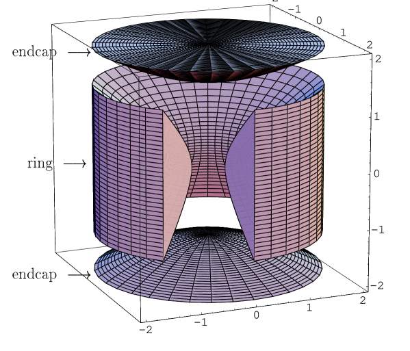
Figure 2: simulation of the Penning trap cavity. The missing section of the ring was removed to see better the inside of the cavity.

The characteristics of the motion can be easily seen by expanding explicitly the previous Hamiltonian:

$$H=H_{z}+H_{c}+H_{\rho},$$

where $H_{z},\ H_{c}$ and $H_{\rho}$ are commuting Hamiltonians given by:

$$\matrix{H_{z}=&\hskip-147.95424pt{1\over 2m}p_{z}^{2}+{m\over 2}\omega_{0}^{2}z^{2},\vskip 6.0pt plus 2.0pt minus 2.0pt\cr H_{c}=&\hskip-184.9429pt-{\omega_{c}\over 2}L_{z},\vskip 6.0pt plus 2.0pt minus 2.0pt\cr H_{\rho}=&{1\over 2m}\left(p_{x}^{2}+p_{y}^{2}\right)+{m\over 2}\omega_{\rho}^{2}\,(x^{2}+y^{2})={1\over 2m}p_{\rho}^{2}+{m\over 2}\omega_{\rho}^{2}\,\rho^{2},}$$

and the trap regime is guaranteed if

$$\omega_{0}^{2}=-{4eV_{0}\over m}>0,\qquad\omega_{c}={eB_{0}\over mc}>0,\qquad\omega_{\rho}^{2}={\omega_{c}^{2}-2\omega_{0}^{2}\over 4}>0.$$

Along $z$ direction we have harmonic oscillator motion of frequency $\omega_{0}$. On the $x-y$ plane the motion consists of rotations around $z$ axis with frequency $\omega_{c}/2$ superposed to a harmonic oscillator motion of frequency $\omega_{\rho}$ along $\rho$. Notice that there are indeed just two independent frequencies.

3.1 Penning loops

We want not only trapping, but to induce some finer manipulations on the system, e.g., the evolution loops. They arise if the three motions $H_{z},\ H_{c},\ H_{\rho}$ are ‘sinchronized’, i.e., if the frequencies $\omega_{0},\ \omega_{c},\ \omega_{\rho}$ are commensurable. There are different possibilities:

• If $\omega_{\rho}/\omega_{0}=l_{2}/l_{1}\in{\bf Q}$, the $z-\rho$ motions can be sinchronized. What is left at $\tau=l_{1}T,\ T=2\pi/\omega_{0}$ are pure rigid rotations

• If $\omega_{c}/\omega_{0}\in{\bf Q}$, it is not guaranteed that $\omega_{\rho}/\omega_{0}$ will be also rational. However, there are some values of $\omega_{c}/\omega_{0}\in{\bf Q}$ for which this happens

  $$\matrix{{\omega_{c}/\omega_{0}}={3/2},&{\omega_{\rho}/\omega_{0}}={1/4},&\tau=2T,\vskip 3.0pt plus 1.0pt minus 1.0pt\cr{\omega_{c}/\omega_{0}}={9/4},&{\omega_{\rho}/\omega_{0}}={7/8},&\tau=4T,\vskip 3.0pt plus 1.0pt minus 1.0pt\cr{\omega_{c}/\omega_{0}}={33/8},&{\omega_{\rho}/\omega_{0}}={31/16},&\tau=8T.}$$

The results above mean that the evolution loops are DAO of the charge inside the Penning trap. We have called them Penning loops (PL) [6].

3.2 Perturbed Penning loops

From now on, let us restrict ourselves to the PL with period $\tau=2T$, i.e., take $\omega_{c}=3\omega_{0}/2,\ \omega_{\rho}=\omega_{0}/4$. Let us ‘perturb’ this PL by a sucession of two instantaneous discharges applied to the walls of the trap, represented by the potential

$$V^{\prime}({\bf r},t)=\left[V_{0}^{\prime}\delta(t-t_{1})+V_{0}^{\prime\prime}\delta(t-t_{2})\right]({\bf r}^{2}-3z^{2})\quad t_{1}<t_{2}<\tau.$$

The total Hamiltonian is again a sum of 3 commuting terms

$$H(t)=H^{l}+eV^{\prime}({\bf r},t)=H_{z}(t)+H_{c}^{l}+H_{\rho}(t),$$

$$H_{z}(t)=H_{z}^{l}+{m\over 2}\left[F^{\prime}\delta(t-t_{1})+F^{\prime\prime}\delta(t-t_{2})\right]z^{2},$$

$$H_{\rho}(t)=H_{\rho}^{l}-{m\over 4}\left[F^{\prime}\delta(t-t_{1})+F^{\prime\prime}\delta(t-t_{2})\right]\rho^{2},$$

$$F^{\prime}=-{4eV_{0}^{\prime}\over m},\qquad F^{\prime\prime}=-{4eV_{0}^{\prime\prime}\over m},$$

where the superindex $l$ means to choose the specific values of $\omega_{0},\ \omega_{c}$ and $\omega_{\rho}$ producing the EL with $\tau=2T$. The evolution operator at $\tau$ takes the factorized form

$$U(\tau)=U_{z}(\tau)U_{c}(\tau)U_{\rho}(\tau),$$

where

$$\matrix{U_{z}(\tau)=&e^{-iH_{z}^{l}(\tau-t_{2})}e^{-iF^{\prime\prime}mz^{2}/2}e^{-iH_{z}^{l}(t_{2}-t_{1})}e^{-iF^{\prime}mz^{2}/2}e^{-iH_{z}^{l}t_{1}},\vskip 6.0pt plus 2.0pt minus 2.0pt\cr U_{c}(\tau)=&\hskip-156.49014pte^{-iH_{c}^{l}\tau}=e^{i3\pi L_{z}},\vskip 6.0pt plus 2.0pt minus 2.0pt\cr U_{\rho}(\tau)=&\hskip-14.22636pte^{-iH_{\rho}^{l}(\tau-t_{2})}e^{iF^{\prime\prime}m\rho^{2}/4}e^{-iH_{\rho}^{l}(t_{2}-t_{1})}e^{iF^{\prime}m\rho^{2}/4}e^{-iH_{\rho}^{l}t_{1}}.}$$

For quadratic Hamiltonians, $U(\tau)$ is defined by the linear transformation

$$U^{\dagger}(\tau)\left(\matrix{{\bf r}\cr{\bf p}}\right)U(\tau)={\bf u}(\tau)\left(\matrix{{\bf r}\cr{\bf p}}\right),$$

where ${\bf u}(t)$ is a $6\times 6$ simplectic matrix called evolution matrix. In our case that matrix reduces to $2\times 2$ unimodular matrices $u_{x}=u_{y}={\bf u}_{x}(\tau)={\bf u}_{y}(\tau)$, $u_{z}={\bf u}_{z}(\tau)$ acting on the pairs $(x,p_{x})^{T}$, $(y,p_{y})^{T}$, $(z,p_{z})^{T}$:

$$\matrix{u_{x}=&\hskip-8.5359pt-u_{ho}({\omega_{0}\over 4},\tau-t_{2})u_{k}(-{F^{\prime\prime}\over 2})u_{ho}({\omega_{0}\over 4},t_{2}-t_{1})u_{k}(-{F^{\prime}\over 2})u_{ho}({\omega_{0}\over 4},t_{1}),\vskip 6.0pt plus 2.0pt minus 2.0pt\cr u_{z}=&\hskip-22.76228ptu_{ho}(\omega_{0},\tau-t_{2})u_{k}(F^{\prime\prime})u_{ho}(\omega_{0},t_{2}-t_{1})u_{k}(F^{\prime})u_{ho}(\omega_{0},t_{1}).}$$

Notice that the evolution matrices $u_{ho}$, $u_{k}$, and the corresponding operators inducing them are of the form:

$$\matrix{u_{ho}(\omega,t)=\left(\matrix{\cos\omega t&{\sin\omega t\over m\omega}\cr-m\omega\sin\omega t&\cos\omega t}\right),&U_{ho}(t)=e^{-i({p^{2}\over 2m}+m\omega^{2}{q^{2}\over 2})t},\vskip 6.0pt plus 2.0pt minus 2.0pt\cr\hskip-34.14322ptu_{k}(F)=\left(\matrix{1&0\cr-mF&1}\right),&\hskip-31.2982ptU_{k}(t_{0})=e^{-imF{q^{2}\over 2}}.}$$

We are interested in the following transformations (the corresponding parameters making them true are immediately reported in the corresponding table):

• 3-dim Fourier-like transformation

  $$\matrix{x\rightarrow\lambda_{2}p_{x}&y\rightarrow\lambda_{2}p_{y}&z\rightarrow\lambda_{1}p_{z}\vskip 3.0pt plus 1.0pt minus 1.0pt\cr p_{x}\rightarrow-{1\over\lambda_{2}}x&p_{y}\rightarrow-{1\over\lambda_{2}}y&p_{z}\rightarrow-{1\over\lambda_{1}}z}$$

  
  

  $\omega_{0}t_{1}$ $\omega_{0}t_{2}$ ${F^{\prime}/\omega_{0}}={F^{\prime\prime}/\omega_{0}}$ $m\omega_{0}\lambda_{1}$ $m\omega_{0}\lambda_{2}$ $5.3131$ $\ 7.2533$ $\ \ 1.5165$ $\ \ 3.5238$ $-39.0332$ $5.3131$ $\ 7.2533$ $-1.5165$ $-0.6046$ $\ \ \ \ 6.6970$ $0.9701$ $11.5962$ $\ \ 1.5165$ $\ \ 0.6046$ $\ \ -2.3891$ $0.9701$ $11.5962$ $-1.5165$ $-3.5238$ $\ \ \ \ 0.4099$

  Table 1. The parameters producing a 3-dim Fourier-like transformation.

• 1-dim Fourier-like transformation in $z$ plus 2-dim scale transformation in $x-y$

  $$\matrix{x\rightarrow\lambda_{2}x&y\rightarrow\lambda_{2}y&z\rightarrow\lambda_{1}p_{z}\vskip 3.0pt plus 1.0pt minus 1.0pt\cr p_{x}\rightarrow{1\over\lambda_{2}}p_{x}&p_{y}\rightarrow{1\over\lambda_{2}}p_{y}&p_{z}\rightarrow-{1\over\lambda_{1}}z}$$

  
  

  $\omega_{0}t_{1}$ $\omega_{0}t_{2}$ ${F^{\prime}/\omega_{0}}={F^{\prime\prime}/\omega_{0}}$ $m\omega_{0}\lambda_{1}$ $\lambda_{2}$ $1.2094$ $\ 5.0738$ $-2.1381$ $-6.3874$ $-10.2781$ $1.9322$ $\ 4.3510$ $-2.1381$ $-1.0959$ $\ \ -3.6353$ $7.4926$ $11.3569$ $-2.1381$ $-6.3874$ $\ \ -0.0973$ $8.2153$ $10.6342$ $-2.1381$ $-1.0959$ $\ \ -0.2751$

  Table 2. The conditions to produce 1-dim Fourier-like and 2-dim scale transformations on $z$ and $x-y$ respectively.

• 3-dim scale transformation

  $$\matrix{x\rightarrow\lambda_{2}x&y\rightarrow\lambda_{2}y&z\rightarrow\lambda_{1}z\vskip 3.0pt plus 1.0pt minus 1.0pt\cr p_{x}\rightarrow{1\over\lambda_{2}}p_{x}&p_{y}\rightarrow{1\over\lambda_{2}}p_{y}&p_{z}\rightarrow{1\over\lambda_{1}}p_{z}}$$

  
  

  $\omega_{0}t_{1}$ $\omega_{0}t_{2}$ ${F^{\prime}/\omega_{0}}$ ${F^{\prime\prime}/\omega_{0}}$ $\lambda_{1}$ $\lambda_{2}$ $1.2363$ $\ 8.4896$ $-1.1589$ $\ \ 0.7524$ $0.4712$ $5.0901$ $2.2064$ $\ 7.5194$ $-0.7524$ $\ \ 1.1589$ $2.1222$ $5.0901$ $4.0768$ $11.3301$ $\ \ 0.7524$ $-1.1589$ $2.1222$ $0.1965$ $5.0469$ $10.3600$ $\ \ 1.1589$ $-0.7524$ $0.4712$ $0.1965$

  Table 3. The parameters inducing the 3-dim scale transformation.

To find the values producing, e.g., the 3-dimensional Fourier-like transformation, we impose that the off diagonal elements of $u_{x}$ and $u_{z}$ of (4) become null. By solving these equations we will find the values of $\omega_{0}t_{1},\ \omega_{0}t_{2},\ F^{\prime}/\omega_{0}$ and $F^{\prime\prime}/\omega_{0}$ inducing that transformation, and from these it is simple to find the corresponding values of the parameters $\lambda_{1}$ and $\lambda_{2}$ (see table 1). The same procedure can be used for the other two transformations (see tables 2 and 3) [6].

We are specially interested in the scale transformation due to its close connection with squeezing. From table 3, it is clear that we can produce different combinations of squeezing and amplification. For instance, if we take the values in the first row, at the end of the full process we will have produced a squeezing with scaling $0.47$ along $z$ direction and an expansion on $x-y$ scaled by $5.09$. By taking the values in the fourth row we will have produced the 3-dimensional squeezing with scalings $0.47$ along $z$ and $0.19$ on $x-y$ plane. It is interesting to notice that a particular scale transformation can also be gotten if

$$\omega_{0}t_{2}=\omega_{0}t_{1}+2\pi,\qquad{F^{\prime\prime}\over\omega_{0}}=-{F^{\prime}\over\omega_{0}}=\cot({\omega_{0}t_{1}\over 2}).$$

The scaling parameters are in this case (see figure 3):

$$\lambda_{1}=1,\qquad\lambda_{2}=\left({1+\cos({\omega_{0}t_{1}\over 2})\over\sin({\omega_{0}t_{1}\over 2})}\right)^{2},\qquad 0<\omega_{0}t_{1}<2\pi.$$

This means that along $z$ direction an EL is again produced but on the $x-y$ plane we have gotten the scale transformation. The squeezing arises when $\omega_{0}t_{1}$ takes values in the interval $(\pi,2\pi)$ with the corresponding kick intensities as given above.

Figure 3: the scale parameter $\lambda_{2}$ as a function of $\zeta=\omega_{0}t_{1}$.

4 Geometric phase

The geometric phase was discovered by Berry, who realized that for cyclic adiabatic evolution of the eigenstates of a slowly changing cyclic Hamiltonian, $H(\tau)=H(0)$, there is associated a geometric phase factor unnoticed by many people that had been working by years with the adiabatic approximation [17]. Later on, Aharonov and Anandan realized that the key point of Berry’s approach was the cyclicity of the state rather than the adiabatic assumption, and thus they associated a geometric phase to any cyclic evolution regardless whether or not the Hamiltonian inducing the evolution changes slowly in time or even if it is time-independent [18]. The most economic formulation of the geometric phase runs as follows [19].

Suppose that a system state $|\psi(t)\rangle$ is cyclic, i.e.

$$|\psi(\tau)\rangle=e^{i\phi}|\psi(0)\rangle.$$

It turns out that $\phi$ is a sum of a dynamic plus a geometric contribution, the last one called geometric phase is given by

$$\beta=\phi+i\int_{0}^{\tau}\langle\psi(t)|{d\over dt}|\psi(t)\rangle dt.$$

$\beta$ is geometric in the sense that it is the holonomy of the horizontal lifting of the closed trajectory in the projective Hilbert space ${\cal P}$, which arises due to the curvature of ${\cal P}$. Hence, $\beta$ measures global curvature effects of the projective Hilbert space. It is worth to notice that the calculation of the geometric phase, even the determination of the cyclic states of a given system, is not an easy task. This is one of the reasons why a lot of people have became involved in the subject [13, 14, 20, 21, 22, 23].

5 Geometric phase and Penning loops

As pointed above, for a system in a Penning loop any state $|\psi(t)\rangle$ is cyclic with period equal to the loop period:

$$|\psi(\tau)\rangle=e^{\phi}|\psi(0)\rangle.$$

Thus, it is quite natural that a geometric phase factor should be associated to any state. For evolution loops induced by time-independent Hamiltonians, the geometric phase is directly related to the expected value of the energy in the initial state:

$$\beta=\phi+\tau\langle\psi(0)|H^{l}|\psi(0)\rangle.$$

An alternative formula arises working in the basis of energy eigenstates of $H^{l}$, where again the superindex $l$ means that we are taking the parameters of $H$ so as to induce the corresponding Penning loop. Let be $|E_{n_{1}n_{2}n_{3}}\rangle$ the eigenstate of $H^{l}$ associated to the eigenvalue $E_{n_{1}n_{2}n_{3}}$:

$$H^{l}|E_{n_{1}n_{2}n_{3}}\rangle=E_{n_{1}n_{2}n_{3}}|E_{n_{1}n_{2}n_{3}}\rangle.$$

By decomposing now $|\psi(0)\rangle$ in that basis

$$|\psi(0)\rangle=\sum_{n_{1}n_{2}n_{3}=0}^{\infty}c_{n_{1}n_{2}n_{3}}|E_{n_{1}n_{2}n_{3}}\rangle,$$

we finally get

$$\beta=\phi+\sum_{n_{1}n_{2}n_{3}=0}^{\infty}E_{n_{1}n_{2}n_{3}}|c_{n_{1}n_{2}n_{3}}|^{2}.$$

This formula is similar to the one obtained for the evolution loop induced by the harmonic oscillator Hamiltonian [14] (see also [13]).

5.1 Geometric phase and perturbed Penning loops

Now, instead of ‘perturbing’ the PL by a term affecting the scalar potential of $H$, as in section 3.2, we perturb its magnetic part so that the static initial magnetic field ${\bf B}_{0}$ becomes the rotating magnetic field [22]:

$${\bf B}(t)=(B\cos\omega t,B\sin\omega t,B_{0}).$$

This system is closer to the systems used by other people to analyse the geometric phase, so it is important to determine its cyclic states. The Hamiltonian can be written

$$H(t)={1\over 2m}\left({\bf p}+{e\over 2c}{\bf r}\times{\bf B}(t)\right)^{2}+{m\over 2}\omega_{0}^{2}\left(z^{2}-{x^{2}+y^{2}\over 2}\right).$$

In order to eliminate the time dependence, let us make the ‘transition to the rotating frame’ [24], i.e., express the evolution operator as follows:

$$U(t)=e^{-i\omega tL_{z}}e^{-iGt},$$

where $G$ is the time-independent Floquet generator:

$$G=H(0)-\omega L_{z}.$$

As $G$ is quadratic in ${\bf v}^{T}=({\bf r},{\bf p})$, the motion is determined by the kind of linear transformation induced on ${\bf v}$ by $e^{-iGt}$:

$${\bf v}(t)=e^{iGt}{\bf v}e^{-iGt}=e^{\Lambda t}{\bf v},\qquad[iG,{\bf v}]=\Lambda{\bf v}.$$

This depends on the roots of the characteristic polynomial of $\Lambda$, ${\rm Det}(\lambda I-\Lambda)$, which become dependent of three dimensionless parameters

$$\alpha={|e|B\over 2mc\omega},\qquad\alpha_{0}={|e|B_{0}\over 2mc\omega}={\omega_{c}\over 2\omega},\qquad w={\omega_{0}\over\omega}.$$

Our interest is centered in the case when all the roots of ${\rm Det}(\lambda I-\Lambda)$ are purely imaginary because in such a case $G$ will induce ‘confined’ motions; this just restricts the parameters $\alpha,\ \alpha_{0},\ w$ to some region in $\alpha-\alpha_{0}-w$ space. By simplicity, we assume that the static fields of the Penning trap induce the PL with period $\tau=2T$, i.e.,

$$\omega_{0}={2\omega_{c}\over 3}\quad\Rightarrow\quad w={2\omega_{c}\over 3\omega}={4\alpha_{0}\over 3}.$$

With this assumption, we can illustrate the classification of the 2-dimensional parameter space $\alpha-\alpha_{0}$ according to the nature of the motion induced on the charged particle (see figure 4). The regions for which the motion is trapped are labelled as $T_{i},\ i=1,\dots,4$, while the rest of the parameter domain produces deconfined motion [22].

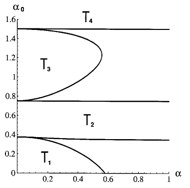
Figure 4: classification of the $\alpha-\alpha_{0}$ plane into regions in which the charged particle performs confined motion (the regions labelled by $T_{i},\ i=1,\dots,4$) and deconfined motion (the rest of the plane).

From now on, let us suppose that the parameters $\alpha$ and $\alpha_{0}$ belong to one of the regions $T_{i},\ i=1,\dots,4$. In such a case, the Floquet generator $G$ becomes the superposition of three harmonic oscillator Hamiltonians:

$$G=\sum_{i=1}^{3}\epsilon_{i}\omega_{i}\left(A_{i}^{\dagger}A_{i}+{\epsilon_{i}\over 2}\right),$$

$$[A_{i},A_{i}^{\dagger}]=\epsilon_{j}\delta_{ij},\qquad\epsilon_{i}=\pm 1.$$

Notice that some of the $\epsilon_{i},i=1,2,3$ could be negative, and in such a case there will be a global minus for the oscillator Hamiltonian contributing to $G$; this will be reflected in the spectrum of $G$ which will not be bounded by below (see also [24]).

Denote the eigenstates of $G$ by $|{\cal E}_{n_{1}n_{2}n_{3}}\rangle$, i.e.

$$G|{\cal E}_{n_{1}n_{2}n_{3}}\rangle={\cal E}_{n_{1}n_{2}n_{3}}|{\cal E}_{n_{1}n_{2}n_{3}}\rangle.$$

Let us assume that

$$|\psi(0)\rangle=|{\cal E}_{n_{1}n_{2}n_{3}}\rangle.$$

The time evolution of this state is very simple:

$$|\psi(t)\rangle=e^{-i\omega tL_{z}}e^{-iGt}|{\cal E}_{n_{1}n_{2}n_{3}}\rangle=e^{-i{\cal E}_{n_{1}n_{2}n_{3}}t}e^{-i\omega tL_{z}}|{\cal E}_{n_{1}n_{2}n_{3}}\rangle.$$

Notice that this state is cyclic with period $\tau=2\pi/\omega$

$$|\psi(\tau)\rangle=e^{-i{\cal E}_{n_{1}n_{2}n_{3}}\tau}|\psi(0)\rangle.$$

Its corresponding geometric phase is easily evaluated

$$\beta_{n_{1}n_{2}n_{3}}=2\pi\langle{\cal E}_{n_{1}n_{2}n_{3}}|L_{3}|{\cal E}_{n_{1}n_{2}n_{3}}\rangle.$$

It is possible to express the previous phase in terms of ${\cal E}_{n_{1}n_{2}n_{3}}$; indeed, we have gotten a beautiful expression [21, 22]:

$$\beta_{n_{1}n_{2}n_{3}}=-2\pi{\partial\over\partial\omega}{\cal E}_{n_{1}n_{2}n_{3}}=-2\pi\sum_{i=1}^{3}\epsilon_{i}\left(n_{i}+{1\over 2}\right){\partial\omega_{i}\over\partial\omega}.$$

Thus, if we change slightly the rotation frequency $\omega$ of the field there will be a slight change in the levels of the Floquet generator $G$. The difference of the new level position and the old one at first order in $\omega$ is essentially the geometric phase.

6 Conclusions

• We have seen that the dynamical manipulation, a procedure which looks for the variety of the operations that can be dynamically induced on a physical system, provides a more global notion of dynamics than the standard one.

• We have seen also that the dynamical manipulation leads in a natural way to the study of some fundamental and practical problems in QM, as the squeezing transformation and the wavepacket reduction in a non-demolishing arrangement.

• Finally, we have seen that those special dynamical processes called evolution loops provide the tools to easily evaluate the geometric phases for the corresponding cyclic evolutions or to simplify their calculation.

References

• [1] W.E. Lamb Jr., Phys. Today 22 (4), 23 (1969)
• [2] E. Lubkin, J. Math. Phys. 15, 673 (1974)
• [3] B. Mielnik, Rep. Math. Phys. 12, 331 (1977)
• [4] J. Waniewski, Commun. Math. Phys. 76, 27 (1980)
• [5] B. Mielnik, J. Math. Phys. 27, 2290 (1986)
• [6] D.J. Fernández C., Nuovo Cim. 107B, 885 (1992)
• [7] P. Brumer and M. Shapiro, Annu. Rev. Phys. Chem. 43, 257 (1992)
• [8] D.J. Fernández C. and B. Mielnik, J. Math. Phys. 35, 2083 (1994)
• [9] D.J. Fernández C. and B. Mielnik, NASA CP 3270, 173 (1994)
• [10] B. Mielnik and D.J. Fernández C., NASA CP 3322, 241 (1996)
• [11] V. Ramakrishna and H. Rabitz, Phys. Rev. A 54, 1715 (1996)
• [12] B. Mielnik, in Field theory, integrable systems and symmetries, F. Khanna and L. Vinet Eds., Les Publications CRM, Montréal (1997), p. 174
• [13] D.J. Fernández C. and O. Rosas-Ortiz, Phys. Lett. A 236, 275 (1997)
• [14] D.J. Fernández C., Int. J. Theor. Phys. 33, 2037 (1994)
• [15] C.M. Caves, K.S. Thorne, R.W.P. Drever, V.D. Sandberg and M. Zimmermann, Rev. Mod. Phys. 52, 341 (1980).
• [16] L.S. Brown and G. Gabrielse, Rev. Mod. Phys. 58, 233 (1986)
• [17] M.V. Berry, Proc. R. Lond. A 392, 45 (1984)
• [18] Y. Aharonov and J. Anandan, Phys. Rev. Lett. 58, 1593 (1987)
• [19] A. Bohm, L.J. Boya and B. Kendrick, Phys. Rev. A 43, 1206 (1991)
• [20] D.J. Fernández C., L.M. Nieto, M.A. del Olmo and M. Santander, J. Phys. A 25, 5151 (1992)
• [21] D.J. Fernández C., M.A. del Olmo and M. Santander, J. Phys. A 25, 6409 (1992)
• [22] D.J. Fernández C. and N. Bretón, Europhys. Lett. 21, 147 (1993)
• [23] J.M. Cerveró and J.D. Lejarreta, J. Phys. A 31, 5507 (1998)
• [24] B. Mielnik and D.J. Fernández C., J. Math. Phys. 30, 537 (1989).