Differential cross section for Aharonov–Bohm effect with non standard boundary conditions

P. Šťovíček, O. Váňa

Department of Mathematics, Faculty of Nuclear Science, CTU,
Trojanova 13, 120 00 Prague, Czech Republic

Abstract

A basic analysis is provided for the differential cross section characterizing Aharonov–Bohm effect with non standard (non regular) boundary conditions imposed on a wave function at the potential barrier. If compared with the standard case two new features can occur: a violation of rotational symmetry and a more significant backward scattering.

PACS. 03.65.Nk – Nonrelativistic scattering theory

The purpose of this letter is to visualize the results of a recent paper [1] in which the dynamics of a non-relativistic spinless quantum particle was studied under the joint effect of a magnetic flux together with a potential barrier shielding a thin, infinite solenoid. The new feature of the mathematical model was that it allowed a general boundary condition imposed on a wave function at the potential barrier. Of course, the traditional regular boundary condition, as introduced by Aharonov and Bohm [2], is included as a particular case. We note that the same subject has been treated independently in [3]. However, the theoretical formulae derived in [1] are complex enough and don’t provide a direct insight into the character of the differential cross section so that one is forced to do some elementary numerical analysis. Thus our main concern here is to discuss the scattering problem and to plot a few graphs. Particularly interesting is the dependence of the differential cross section on the type of boundary condition, and it will be actually shown to be non trivial. In addition, we were able to simplify the mentioned formulae in some particular cases.

We consider the idealized setup when the radius of the solenoid goes to zero while the value $\phi$ of the flux of the magnetic field is kept constant. Moreover, owing to the translational symmetry in the direction of the solenoid the problem reduces immediately to two dimensions. As usual, we denote respectively by $m,\ e$ and $E$ the mass, the electric charge, and the energy of the scattering particle, and we set $k=(2mE/\hbar^{2})^{1/2}$.

In [1] a five-parameter family of Hamilton operators was described. One of the parameters is related directly to the flux. Namely, we shall use the rescaled quantity

$$\alpha:=-e\phi/2\pi\hbar c\quad\mbox{with}\quad\alpha\in(0,1).$$ (1)

The restriction of the range of $\alpha$ is possible due to the gauge symmetry [4]. Actually, as is well known, the quantum particle cannot distinguish between two fluxes which differ by an integer multiple of $2\pi\hbar c/e$. Moreover, we have excluded the value $\alpha=0$ corresponding to the vanishing magnetic flux. The remaining four parameters determine boundary conditions imposed on the wave function at the origin, and should be related in some way to the strength and quality of the potential barrier. As already mentioned, the usual Aharonov-Bohm (AB) effect [2] corresponds to the regular boundary condition, and, for the sake of simplicity, we shall call it the pure AB effect.

Let us now describe the family of Hamilton operators explicitly. All of them are the usual differential operators in the polar coordinates $r,\ \theta$ :

$$-\frac{\hbar^{2}}{2m}\left({\partial^{2}\over\partial r^{2}}+{1\over r}~{}{\partial\over\partial r}+{1\over r^{2}}~{}\left({\partial\over\partial\theta}+\imath\alpha\right)^{2}\right).$$ (2)

To specify the boundary conditions we first introduce the quantities $\Phi_{k}^{j}(\psi)$, $j,k=1,2$, describing the asymptotic behavior of a wave function $\psi$ at the origin:

$$\Phi_{1}^{1}(\psi) := \lim_{r\to 0}~{}r^{1-\alpha}\int_{0}^{2\pi}\psi(r,\theta)\,e^{\imath\theta}\,d\theta/2\pi\,,$$

$$\Phi_{2}^{1}(\psi) := \lim_{r\to 0}~{}r^{-1+\alpha}\left[\int_{0}^{2\pi}\psi(r,\theta)\,e^{\imath\theta}\,d\theta/2\pi-r^{-1+\alpha}\Phi_{1}^{1}(\psi)\right]\,,$$ (3)

$$\Phi_{1}^{2}(\psi) := \lim_{r\to 0}~{}r^{\alpha}\int_{0}^{2\pi}\psi(r,\theta)\,d\theta/2\pi\,,$$

$$\Phi_{2}^{2}(\psi) := \lim_{r\to 0}~{}r^{-\alpha}\left[\int_{0}^{2\pi}\psi(r,\theta)\,d\theta/2\pi-r^{-\alpha}\Phi_{1}^{2}(\psi)\right]\,.$$

The boundary conditions then read

$$\pmatrix{\Phi_{1}^{1}(\psi)\cr\Phi_{1}^{2}(\psi)}=\pmatrix{u^{\prime}&\alpha\bar{w^{\prime}}\cr(1\!-\!\alpha)w^{\prime}&v^{\prime}}\pmatrix{\Phi_{2}^{1}(\psi)\cr\Phi_{2}^{2}(\psi)}$$ (4)

where $u^{\prime},v^{\prime}\in\mathbb{R}$ and $w^{\prime}\in\mathbb{C}$ represent altogether four real parameters. Particularly the pure AB effect corresponds to the values $u^{\prime}=v^{\prime}=0$ and $w^{\prime}=0$. We note also that the boundary conditions (4) are rotationally invariant only if $w^{\prime}=0$. So generally the angular momentum is not conserved.

To make simpler the formulae presented below we will use the dimensionless parameters

$$u:=\frac{\Gamma(\alpha)}{\Gamma(2-\alpha)}\left({k\over 2}\right)^{2-2\alpha}\,u^{\prime},\ v:=\frac{\Gamma(1-\alpha)}{\Gamma(1+\alpha)}\left({k\over 2}\right)^{2\alpha}\,v^{\prime},\ w:={k\over 2}\,w^{\prime}.$$ (5)

But one has to keep in mind that $u,\ v$ and $w$ now depend on the momentum $k$ and that the true parameters fixing the Hamilton operator are the original ones, i.e., $u^{\prime},\ v^{\prime}$ and $w^{\prime}$.

Let us recall that the differential cross section in the plane is given by the equality

$$\frac{d\sigma(\theta)}{d\theta}={2\pi\over k}|S(k;\theta,\theta_{0})|^{2}$$ (6)

where $S(k;\theta,\theta_{0})$ is the scattering matrix. The angle $\theta_{0}$ determines the direction of motion of the incident particle and it is generally of importance because of the violation of rotational symmetry when $w\neq 0$. In fact, if the problem was rotationally symmetric the angles $\theta$ and $\theta_{0}$ would occur in the expression for $S(k;\theta,\theta_{0})$ only in the combination $\theta-\theta_{0}$ which need not be the case as we shall see. Thus one has to consider the dependence of the differential cross section altogether on six real parameters: $u,\ v,\ \mbox{Re }w,\ \mbox{Im }w,\ \alpha$ and $\theta_{0}$.

For the scattering matrix the following formula has been derived:

$$S(k;\theta,\theta_{0}) = \cos(\pi\alpha)\,\delta(\theta\!-\!\theta_{0})+{1\over 2\pi}\sin(\pi\alpha)\frac{e^{-\imath(\theta-\theta_{0})/2}}{\sin\bigl{(}(\theta-\theta_{0})/2\bigr{)}}$$

$$+{1\over 2\pi}\left((\Sigma_{11}-e^{\imath\pi\alpha})e^{-\imath(\theta-\theta_{0})}+\Sigma_{12}\,e^{-\imath\theta}+\Sigma_{21}\,e^{\imath\theta_{0}}+\Sigma_{22}-e^{-\imath\pi\alpha}\right)$$

where

$$\Sigma_{11} = {\det}^{-1}N(k)\,\left(e^{-\imath\pi\alpha}\left(uv-|w|^{2}\right)+u-v-e^{\imath\pi\alpha}\right),$$

$$\Sigma_{12} = -{\det}^{-1}N(k)\,2\imath\,\sin(\pi\alpha)~{}\bar{w},$$

$$\Sigma_{21} = -{\det}^{-1}N(k)\,2\imath\,\sin(\pi\alpha)~{}w,$$ (8)

$$\Sigma_{22} = {\det}^{-1}N(k)\,\left(e^{\imath\pi\alpha}\left(uv-|w|^{2}\right)+u-v-e^{-\imath\pi\alpha}\right),$$

and

$$\det N(k)=uv-|w|^{2}+e^{\imath\pi\alpha}\,u-e^{-\imath\pi\alpha}\,v-1.$$ (9)

Concerning the differential cross section, after some manipulations we arrive at the expression

$$\frac{d\sigma(\theta)}{d\theta}=\frac{2\sin^{2}(\pi\alpha)}{\pi k}\left|\frac{1}{2\sin\bigl{(}(\theta-\theta_{0})/2\bigr{)}}-\frac{1}{uv-|w|^{2}+e^{\imath\pi\alpha}\,u-e^{-\imath\pi\alpha}\,v-1}\right.$$

$$\times\left(2\sin\bigl{(}(\theta-\theta_{0})/2\bigr{)}(uv-|w|^{2})+\imath\,e^{\imath\bigr{(}\pi\alpha-(\theta-\theta_{0})/2\bigl{)}}\,u\right.$$ (10)

$$\left.\left.+\imath\,e^{-\imath\bigr{(}\pi\alpha-(\theta-\theta_{0})/2\bigl{)}}\,v+2\imath\,\mbox{Re}\biggl{(}e^{\imath(\theta+\theta_{0})/2}\,w\biggr{)}\right)\right|^{2}.$$

Let us proceed to the discussion of the behavior of the function $2\pi|S(k;\theta,\theta_{0})|^{2}$. For the sake of convenience, in the graphs presented below this function depends on the angle $\Theta=\theta-\theta_{0}+\pi$ (mod $2\pi$) rather than directly on $\theta$. Hence the values $\Theta=0$ and $\Theta=-\pi$ correspond to the backward and forward scattering, respectively.

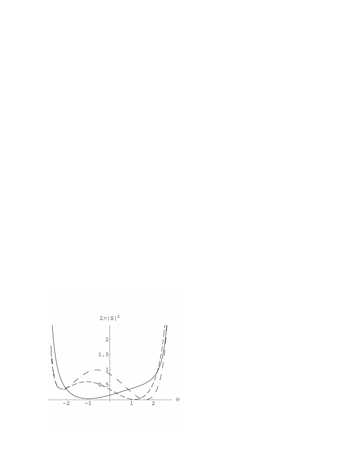
Figure 1: Dependance of $2\pi|S(k;\theta,\theta_{0})|^{2}$ on $\Theta=\theta-\theta_{0}+\pi$ (mod $2\pi$), the solid line corresponds to $u=25$, $v=1$, $w=3+3\imath$ , the dashed line corresponds to $u=20$, $v=0$, $w=3$, the dot-dashed line corresponds to $u=1$, $v=10$, $w=0$, and $\alpha=0.5$, $\theta_{0}=0$ in all three cases.

On Figure 1 we show graphs for three different boundary conditions which have been chosen rather accidentally, and in all three cases $\alpha=0.5$ and $\theta_{0}=0$. As one can observe, there is a common feature which is independent of the boundary conditions and of the angle $\theta_{0}$. The differential cross section is divergent for $\Theta$ tending to $\pm\pi$ (forward scattering). The explanation is simple. The considered problem is somewhat inconsistent from the physical point of view as the total magnetic flux passing through the plane is nonzero. A more consistent arrangement would involve two parallel solenoids with equal fluxes but oppositely oriented [5]. In this case the divergence is actually removed, as discussed in [6].

Further, a rough inspection of the graphs leads to the conclusion that there are two possible shapes. Either the graph exhibits one minimum as in the pure AB effect or there are two local minima and one local maximum. The latter shape takes place for some non-standard boundary conditions and implies existence of a small and rather flat peak centered closely at the value $\Theta=0$. This suggests that, at least in principle, one should be able to detect the boundary conditions describing the physical situation when looking at the backward scattering picture.

To illustrate this observation let us now consider more closely the particular case with $u=v=0$. Then the formulae simplify significantly. It is convenient to write $w$ in the polar form, $w=\rho\exp(\imath\varphi)$. The differential cross section then reads

$$\frac{d\sigma(\theta)}{d\theta} = \frac{\sin^{2}(\pi\alpha)}{2\pi k}$$

$$\times\left(\frac{1}{\sin^{2}\bigl{(}(\theta-\theta_{0})/2\bigr{)}}+8\frac{\rho^{2}}{(1+\rho^{2})^{2}}\left(\cos(\theta+\theta_{0}+2\varphi)-\cos(\theta-\theta_{0})\>\rho^{2}\right)\right).$$

The value $w=0$ corresponds to the pure AB effect, and then

$$\frac{d\sigma_{\mbox{\scriptsize pure}}(\theta)}{d\theta}=\frac{\sin^{2}(\pi\alpha)}{2\pi k\sin^{2}\bigl{(}(\theta-\theta_{0})/2\bigr{)}}\,.$$ (12)

Let us note that though the differential cross section diverges and so the total cross section is not well defined one can take the pure AB effect for the reference point and integrate the difference of the differential cross sections. The result is obviously

$$\int_{0}^{2\pi}\left(\frac{d\sigma(\theta)}{d\theta}-\frac{d\sigma_{\mbox{\scriptsize pure}}(\theta)}{d\theta}\right)\,d\theta=0.$$ (13)

As one can see from (11), the magnetic flux enters the formula in the form of a prefactor $\sin^{2}(\pi\alpha)$. The dependence on the initial angle $\theta_{0}$ as well as on the argument $\varphi$ of $w$ is rather weak. However there is a remarkable difference in the shape of the graph for $w=0$ and $|w|$ large. Actually it is not difficult to calculate the limit of the differential cross section for $|w|\to\infty$ (with $u=v=0$). This way we get the formula

$$\frac{d\sigma_{|w|\to\infty}(\theta)}{d\theta}=\frac{\sin^{2}(\pi\alpha)\left(1-2\cos(\theta-\theta_{0})\right)^{2}}{2\pi k\sin^{2}\bigl{(}(\theta-\theta_{0})/2\bigr{)}}\,.$$ (14)

This limit procedure can be interpreted in two ways. Either one assumes that $u^{\prime}=v^{\prime}=0$, $w^{\prime}$ is fixed and the energy of the particle is large, or that the energy is constant while $|w^{\prime}|\to\infty$ (c.f. (5)). As one finds immediately from (4), the latter interpretation corresponds to the boundary conditions

$$\Phi_{2}^{1}(\psi)=\Phi_{2}^{2}(\psi)=0.$$ (15)

Let us compare the formula (14) with the analogous formula (12) for the pure AB effect. Figure 2 depicts the two graphs.

Let us now examine another particular case, this time with $u=v=w>0$, hence $uv-|w|^{2}=0$. Then we have

$$\frac{d\sigma(\theta)}{d\theta} = \frac{\sin^{2}(\pi\alpha)}{2\pi k\sin^{2}\bigl{(}(\theta-\theta_{0})/2\bigr{)}}$$

$$\times\frac{1+4\big{(}\sin\theta-\sin\theta_{0}-\sin(\pi\alpha-\theta+\theta_{0})\big{)}^{2}\,u^{2}}{1+4\sin^{2}(\pi\alpha)\>u^{2}}\,.$$

Here we can demonstrate a clear violation of the rotational symmetry. Indeed, the three-dimensional plot given in Figure 3 illustrates its rather strong dependence on the initial angle $\theta_{0}$.

This case also indicates that the equality (13) need not be true in general. Comparing again the differential cross section (16) to that one related to the pure AB effect we obtain

$$\frac{d\sigma(\theta)}{d\theta}-\frac{d\sigma_{\mbox{\scriptsize pure}}(\theta)}{d\theta}=\frac{\sin^{2}(\pi\alpha)\,u^{2}}{\pi k(1+4\sin^{2}(\pi\alpha)\,u^{2})}\left(f(\alpha,\theta,\theta_{0})-\frac{\cos^{3}\bigl{(}(\theta-\theta_{0})/2\big{)}}{\sin\bigl{(}(\theta-\theta_{0})/2\bigr{)}}\right)$$ (17)

where

$$f(\alpha,\theta,\theta_{0}) = 8\cos(\pi\alpha)\>(\cos(\pi\alpha)+\cos\theta_{0})+7\cos(\pi\alpha-\theta)+\cos(\pi\alpha+\theta)$$

$$-2\sin(\pi\alpha)\>\sin(\theta-2\theta_{0})+\cos(2\pi\alpha+\theta-\theta_{0})$$

$$+3\cos(2\pi\alpha-\theta+\theta_{0})+4\cos(\theta+\theta_{0})\,.$$

Even this expression still contains a nonintegrable singularity, namely the term $\cos^{3}\bigl{(}(\theta-\theta_{0})/2\bigr{)}/\sin\bigl{(}(\theta-\theta_{0})/2\bigr{)}$. However since this function is $2\pi$ periodic and odd with respect to the point $\theta_{0}$ we can set its integral over an interval of length $2\pi$ equal 0. With this assumption we find that

$$\int_{0}^{2\pi}\left(\frac{d\sigma(\theta)}{d\theta}-\frac{d\sigma_{\mbox{\scriptsize pure}}(\theta)}{d\theta}\right)\,d\theta=\frac{16\sin^{2}(\pi\alpha)\cos(\pi\alpha)\big{(}\cos(\pi\alpha)+\cos\theta_{0}\big{)}\,u^{2}}{k(1+4\sin^{2}(\pi\alpha)\,u^{2})}$$ (19)

which generally need not vanish.

Finally let us consider the case with conserved angular momentum which means that $w=0$. Then the differential cross section equals

$$\frac{d\sigma(\theta)}{d\theta}=\frac{\sin^{2}(\pi\alpha)\>g(u,v,\theta,\theta_{0})}{2\pi k\sin^{2}\bigl{(}(\theta-\theta_{0})/2\bigr{)}\bigl{(}1+u^{2}-2u\cos(\pi\alpha)\bigr{)}\bigl{(}1+v^{2}+2v\cos(\pi\alpha)\bigr{)}}$$ (20)

where

$$g(u,v,\theta,\theta_{0}) = (1+u^{2})(1+v^{2})+4uv\sin^{2}(\pi\alpha-\theta+\theta_{0})+4u^{2}v^{2}\cos^{2}(\theta-\theta_{0})$$ (21)

$$-2(u-v)(1+uv)\cos(\pi\alpha-\theta+\theta_{0})-4uv(1+uv)\cos(\theta-\theta_{0})$$

$$+4(u-v)uv\cos(\pi\alpha-\theta+\theta_{0})\cos(\theta-\theta_{0})\,.$$

Specializing even more, namely setting $u=v$ and $\alpha=1/2$, we get

$$\frac{d\sigma(\theta)}{d\theta}=\frac{1+u^{2}\left(1-2\cos(\theta-\theta_{0})\right)^{2}}{2\pi k\left(1+u^{2}\right)\,\sin^{2}\bigl{(}(\theta-\theta_{0})/2\bigr{)}}$$ (22)

This expression quite resembles the case with $u=v=0$, $w\neq 0$, particularly the limit procedure $u\to\infty$ leads again to the formula (14) (but with $\alpha=1/2$).

This concludes our brief analysis of the differential cross section in dependence on the choice of parameters characterizing the nature of the potential barrier. In fact, it would be not difficult for anyone interested in to reexamine or prolong this analysis when starting from the formula (10). Basically we have demonstrated two new features which may occur: a more significant backward scattering (c.f. Fig. 2) and a violation of rotational symmetry (c.f. Fig. 3).

Acknowledgements. P.S. wishes to gratefully acknowledge the partial support from Grant No. 202/96/0218 of Czech GA.

Figures

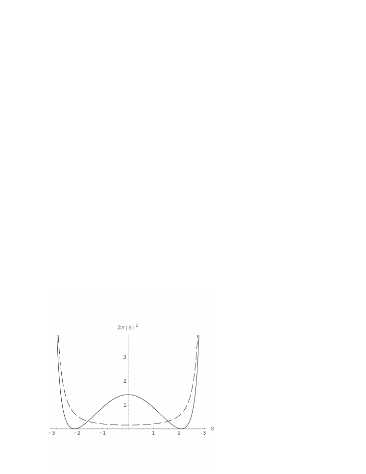
Figure 2: Dependance of $2\pi|S(k;\theta,\theta_{0})|^{2}$ on $\Theta=\theta-\theta_{0}+\pi$ (mod $2\pi$), the solid line corresponds to (14) , the dashed line corresponds to (12), $\alpha=0.5$, and $\theta_{0}$ can be arbitrary.

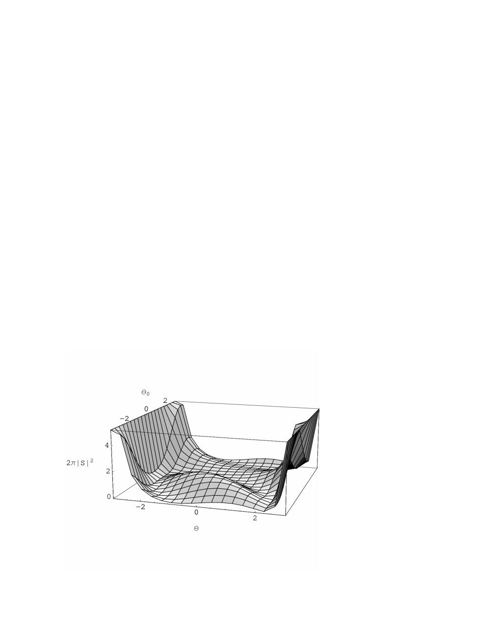
Figure 3: Dependance of $2\pi|S(k;\theta,\theta_{0})|^{2}$ on $\Theta=\theta-\theta_{0}+\pi$ (mod $2\pi$) and $\theta_{0}$ for $u=v=w=5$, , $\alpha=0.5$.

References

[1]Da̧browski L. and Šťovíček P.,
J. Math. Phys. 39 (1998) 47.
[2]Aharonov Y. and Bohm D.,
Phys. Rev. 115 485 (1959).
[3]Adami R. and Teta A.,
Lett. Math. Phys. 43 (1998) 43.
[4]Ruiseenars S.N.M.,
Ann. Phys. 146 (1983) 1.
[5]Peshkin M., Talmi I. and Tassie J.,
Ann. Phys. (N.Y.) (1961) 426.