Reasoning about Grover’s Quantum Search Algorithm using Probabilistic wp

Abstract

Grover’s search algorithm is designed to be executed on a quantum mechanical computer. In this paper, the probabilistic wp-calculus is used to model and reason about Grover’s algorithm. It is demonstrated that the calculus provides a rigorous programming notation for modelling this and other quantum algorithms and that it also provides a systematic framework of analysing such algorithms.

1 Introduction

Quantum computers are a proposed means of using quantum mechanical effects to achieve efficient computation. Quantum mechanical systems may be in superpositions of several different states simultaneously. The central idea of quantum computers is to perform operations on these superposed states simultaneously and thus achieve a form of parallel computation. These devices were proposed in the early 1980’s [Benioff, 1980, Deutsch, 1985].

One essential phenomenon of quantum mechanics is that the measurement of a superposed system forces it into a single classical state. Each superposed state is present with a certain amplitude and an observation causes it to collapse to that state with a probability that depends on its amplitude. This means that, although many computations may be performed in parallel on a quantum device, the result of only one of these may be observed. This may seem like a severe limitation, but several ingenious algorithms have been devised which work by increasing the amplitude of the desired outcome before any observation is performed and thus increasing the likelihood of the observed outcome being the desired one.

One such algorithm is Grover’s quantum search algorithm [Grover, 1997] which performs a search on an unstructured search space of size $N$ in ${\cal O}(\sqrt{N})$ steps. To find the desired search value with 100% probability in such a space, a classical computer cannot do better than a linear time search. Grover’s algorithm performs operations on a superposition of all possible search values that serve to increase the amplitude of the desired search value. Grover shows that within ${\cal O}(\sqrt{N})$ steps there is a greater than 50% chance of finding the desired search value. [Boyer et al., 1998] proved a stronger result for the algorithm showing that the correct search value can be found in ${\cal O}(\sqrt{N})$ with almost 100% probability.

In this paper, we apply the probabilistic weakest-precondition (wp) calculus of [Morgan et al., 1996] to Grover’s algorithm to redevelop the result of [Boyer et al., 1998] in a more systematic way. The probabilistic wp-calculus is an extension of Dijkstra’s standard wp-calculus [Dijkstra, 1976] developed for reasoning about the correctness of imperative programs. The extension supports reasoning about programs containing probabilistic choice. The measurement of a quantum superposition is an example of a probabilistic choice.

Use of the probabilistic wp-calculus contributes two essential ingredients to the analysis of quantum algorithms. Firstly it provides an elegant and rigorous programming language for describing quantum algorithms. The existing literature uses block diagrams and structured English which can be cumbersome and potentially ambiguous. Secondly, the probabilistic wp-calculus provides a set of rules for the systematic analysis of the correctness of algorithms. In the case of standard algorithms, the calculus is used to determine whether a program achieves some desired outcome. In the case of probabilistic algorithms, the calculus is used to reason about the probability of a program achieving some desired outcome.

This paper is not simply about re-presenting a known result about Grover’s algorithm but it also aims to demonstrate that the probabilistic wp-calculus is suitable for both modelling and reasoning about a quantum algorithm. Boyer et al have already derived the same result that we derive here but they do so in a less systematic way. Our hope is that the approach used here could be applied fruitfully to other quantum algorithms and may even aid the development of new quantum algorithms.

The paper is organised as follows. In Section 2, we give a sufficient overview of quantum theory. In Section 3, we present our approach to modelling quantum computation using the programming language of the probabilistic wp-calculus. In Section 4, we present Grover’s algorithm using the approach of Section 3. In Section 5, we give a sufficient introduction to the rules of the probabilistic wp-calculus and in Section 6, we use the wp-calculus to derive a formula for the probability of success of Grover’s algorithm.

2 Quantum Systems and Qubits

In quantum mechanics, a superposition of two states $A$ and $B$ is represented in Dirac’s notation as follows:

$$S = \alpha|A\rangle~{}+~{}\beta|B\rangle.$$

System $S$ is said to be in a superposition of $A$ and $B$. $|A\rangle$ and $|B\rangle$ are the basis states and $\alpha$ and $\beta$ are amplitudes. The amplitudes may be complex numbers.

Let $|\!|z|\!|^{2}$ be the square norm of complex number $z$. Observation of $S$ will cause the system to collapse to state $|A\rangle$ with probability $|\!|\alpha|\!|^{2}$ and to $|B\rangle$ with probability $|\!|\beta|\!|^{2}$. The probabilities must sum to 1:

$$|\!|\alpha|\!|^{2}~{}+~{}|\!|\beta|\!|^{2} = 1.$$

A qubit is a two state quantum system in which the basis states are labelled 0 and 1:

$$S = \alpha|0\rangle~{}+~{}\beta|1\rangle.$$

A classical bit has $\alpha=1$ and $\beta=0$ or $\alpha=0$ and $\beta=1$.

A qubit evolves from one superposition to another using a quantum gate (or function) $F$:

$$F(~{}\alpha|0\rangle~{}+~{}\beta|1\rangle~{}) = \alpha^{\prime}|0\rangle~{}+~{}\beta^{\prime}|1\rangle.$$

$F$ must be unitary which means that

• probabilities are preserved: $|\!|\alpha^{\prime}|\!|^{2}~{}+~{}|\!|\beta^{\prime}|\!|^{2}~{}~{}=~{}~{}|\!|\alpha|\!|^{2}~{}+~{}|\!|\beta|\!|^{2}$, and

• $F$ has an inverse.

In quantum mechanics, a transformation $F$ is usually modelled using matrix multiplication:

$$F(~{}\alpha|0\rangle~{}+~{}\beta|1\rangle~{}) = U_{F}\times\left(\begin{array}[]{l}\alpha\\ \beta\end{array}\right),$$

where $U_{F}$ is a $2\times 2$ unitary matrix. Matrix $U$ is unitary if $U.U^{\dagger}=U^{\dagger}.U=I$ where $U^{\dagger}$ is the conjugate transpose of $U$. It can be shown that such a transformation defined by unitary matrix $U_{F}$ is unitary [Bernstein and Vazirani, 1993].

A quantum superposition may have an arbitrary number of basis states, not just two. An $N$-state superposition is represented as:

$$S = \sum_{i=0}^{N-1}\alpha_{i}|i\rangle.$$

Observation of $S$ will cause it to collapse to state $|i\rangle$ with probability $|\!|\alpha_{i}|\!|^{2}$. Again, the probabilities must sum to 1:

$$\sum_{i=0}^{N-1}|\!|\alpha_{i}|\!|^{2} = 1.$$

A quantum register is a collection of qubits and an $L$-qubit register gives rise to a system with $2^{L}$ basis states. Like qubits, quantum registers evolve under unitary transformations.

For further details on quantum computation, the reader is referred to papers such as [Berthiaume, 1996, Ekert, 1994].

3 Modelling Quantum Computers

A quantum computer is a collection of quantum registers and quantum gates. In this section, we introduce ways of modelling various aspects of quantum computation using the programming language of the probabilistic wp-calculus. We use a subset of the language which includes standard assignment, probabilistic assignment, sequential composition and simple loops.

Firstly, we model an $N$-state quantum system as a function from state indices to complex numbers: $S:(0..N-1)\rightarrow{\mathbb C}$.

A superposition of the form

$$\sum_{i=0}^{N-1}\alpha_{i}|i\rangle$$

is modelled by the function $S$ where for $0\leq i<N$:

$$S(i) = \alpha_{i}.$$

A classical state $i$ is modelled by the function which is zero everywhere except at $i$ which we write as $|i\rangle$:

$$|i\rangle(j) = 1,~{}\hbox{if}~{}i=j$$

$$= 0,~{}\hbox{otherwise}.$$

Transformation of a quantum state is modelled by a standard assignment statement:

$$S~{}:=~{}F(S).$$

$F$ must be unitary for this to be a valid quantum transformation.

We shall find it convenient to use lambda abstraction to represent transformations: $(\lambda i~{}|~{}0\leq i<N\cdot E)$ represents the function that takes an argument $i$ in the range $0..N-1$ and returns the value $E$. For example, the unitary transformation that inverts the amplitude of each basis state is modelled as follows:

$$S~{}:=~{}(~{}\lambda i~{}|~{}0\leq i<N\cdot-S(i)~{}).$$

Sequencing of transformations is modelled using sequential composition: let $T_{1}$ and $T_{2}$ be transformations, then their sequential composition is written $T_{1};T_{2}$.

The loop which iterates $C$ times over a transformation $T$ is written ${\bf do}~{}C~{}{\bf times}~{}T~{}{\bf od}$.

We model the observation of a quantum system using a probabilistic assignment statement. In the simple case, this is a statement of the form:

$$x := E~{}~{}@~{}~{}p,$$

$$F~{}~{}@~{}~{}(1-p).$$

This says that $x$ takes the value $E$ with probability $p$ and the value $F$ with probability $1-p$. For example, a coin flip is modelled by

$$coin := head~{}~{}@~{}~{}0.5,$$

$$tail~{}~{}@~{}~{}0.5.$$

Observation of a two state superposition forces the system into a classical state. This is modelled with the following probabilistic assignment:

$$S := |0\rangle~{}~{}@~{}~{}|\!|S(0)|\!|^{2},$$

$$|1\rangle~{}~{}@~{}~{}|\!|S(1)|\!|^{2}.$$

A generalised probabilistic statement has the form

$$x := E_{i}~{}~{}@~{}~{}p_{i},~{}~{}~{}0\leq i<N,$$

where $(\sum_{i=0}^{N-1}p_{i})=1$.

Now observation of an $N$-state quantum system $S$ may be modelled by

$$S := |i\rangle~{}~{}@~{}~{}|\!|S(i)|\!|^{2},~{}~{}~{}0\leq i<N.$$

That is, $S$ collapses to the classical state $i$ with probability $|\!|S(i)|\!|^{2}$.

4 Grover’s Search Algorithm

The Grover search problem may be stated as follows:

Given a function $f:(0..N-1)\rightarrow\{0,1\}$ that is zero everywhere except for one argument $x_{0}$, where $f(x_{0})=1$, find that argument $x_{0}$.

The algorithm makes use of the mean of a superposition $S$, written $\overline{S}$, where

$$\overline{S} = \frac{\sum_{i=0}^{N-1}S(i)}{N}.$$

$$\begin{array}[]{ll}S~{}:=~{}(\lambda i~{}|~{}0\leq i<N\cdot\frac{1}{\sqrt{N}})~{};&\hbox{ ~{}~{}~{}{Init} }\\[6.45831pt] {\bf do}~{}C~{}{\bf times}\\[4.30554pt] ~{}~{}~{}~{}\begin{array}[]{l}S~{}:=~{}(\lambda i~{}|~{}0\leq i<N\cdot S(i)-2.f(i).S(i)~{})~{};\\[4.30554pt] S~{}:=~{}(\lambda i~{}|~{}0\leq i<N\cdot 2.\overline{S}-S(i)~{})\end{array}&\hbox{ ~{}~{}~{}{Body} }\\[4.30554pt] {\bf od}~{};\\[6.45831pt] S~{}:=~{}|i\rangle~{}~{}@~{}~{}|\!|S(i)|\!|^{2},~{}~{}~{}~{}0\leq i<N&\hbox{ ~{}~{}~{}{Measure} }\end{array}$$

Figure 1: Grover’s search algorithm.

The algorithm is represented in the programming language of the probabilistic wp-calculus in Fig. 1. The initialisation of this algorithm sets the system $S$ up in an equal superposition of all possible basis states. Successive iterations of the loop then serve to increase the amplitude of the search argument $x_{0}$ while decreasing the amplitude of the other arguments. To see why this is so, consider the case of $N=8$. The initialisation sets $S$ up in an equal superposition of the eight possible states, represented diagrammatically as follows:

The first step of the loop body replaces each $S(i)$ with $S(i)-2.f(i).S(i)$. This inverts $S(i)$ about the origin in the case that $f(i)=1$ and leaves $S(i)$ unchanged in the case that $f(i)=0$. Assuming that $f(4)=1$, this replaces our example superposition with

The second step of the loop body inverts each amplitude about the average of all the amplitudes resulting in:

The amplitude of state $|4\rangle$ has increased as a result of the two steps of the loop body, while the amplitude of the others has decreased.

After an optimum number of iterations, $C$, the amplitude of $|x_{0}\rangle$ approaches 1 while the amplitude of the other states approaches 0. An observation is then performed. Since the amplitude of $|x_{0}\rangle$ approaches 1, the probability of the observation yielding $|x_{0}\rangle$ is close to 1. $C$ depends on the number of states $N$ and, as discussed in the next section, it is ${\cal O}(\sqrt{N})$.

5 Probabilistic wp

In two-valued logic, a predicate may be modelled as a function from some state space to the set $\{0,1\}$. For example, the predicate $x>y$ evaluates to $1$ in a state in which $x$ is greater then $y$ and evaluates to $0$ in any other state. A probabilistic predicate generalises the range to the continuous space between $0$ and $1$ [Morgan et al., 1996]. For example, the probabilistic predicate $0.5\times(x>y)$ evaluates to $0.5$ in a state in which $x$ is greater then $y$ and evaluates to $0$ in any other state.

In the standard wp-calculus, the semantics of imperative programs is given using weakest-precondition formulae: for program $prog$ and postcondition $post$, $wp(prog,post)$ represents the weakest precondition (or maximal set of initial states) from which $prog$ is guaranteed to terminate and result in a state satisfying $post$.

The wp rule for assignment is given by:

$$wp(~{}x:=E,~{}post~{}) = post[x/E].$$ (4)

Here, $post[x/E]$ represents predicate $post$ with all free occurrences of $x$ replaced by $E$. For example,

$$wp(x:=7,~{}x>y) = x>y~{}[x/7]$$

$$= 7>y.$$

That is, the assignment $x:=7$ is guaranteed to establish $x>y$ provided $7>y$ initially.

The wp rule for sequential composition is given by:

$$wp(~{}prog1;prog2,~{}post~{}) = wp(~{}prog1,~{}wp(prog2,~{}post~{})~{}).$$ (5)

Both of these rules also apply in the probabilistic wp-calculus. The wp rule for simple probabilistic assignment [Morgan et al., 1996] is given by:

$$wp(~{}x~{}:=~{}E~{}@~{}p,~{}F~{}@~{}1-p~{},~{}~{}post~{})~{}=$$ (6)

$$p\times post[x/E]~{}+~{}(1-p)\times post[x/F].$$

In the case of non-probabilistic $post$, $wp(prog,post)$ represents the probability that program $prog$ establishes $post$. For example

$$wp(~{}coin~{}:=~{}head~{}@~{}0.5,~{}tail~{}@~{}0.5,~{}~{}coin=head~{})$$

$$=$$ by (6)

$$0.5\times(coin=head~{}[coin/head])~{}+~{}0.5\times(coin=head~{}[coin/tail])$$

$$=$$ substitution

$$0.5\times(head=head)~{}+~{}0.5\times(tail=head)$$

$$= 0.5\times 1~{}+~{}0.5\times 0$$

$$= 0.5.$$

That is, a coin flip establishes $coin=head$ with probability $0.5$.

The wp rule for the generalised probabilistic assignment is given by:

$$wp(~{}x~{}:=~{}E_{i}~{}@~{}p_{i},~{}0\leq i<N,~{}~{}post~{}) = \sum_{i=0}^{N-1}p_{i}\times post[x/E_{i}].$$ (7)

The only other programming construct we need in order to model Grover’s algorithm is the DO-loop. Since the algorithm only loops a constant and finite number of times, we can model ${\bf do}~{}C~{}{\bf times}~{}prog~{}{\bf od}$ as a finite sequential composition of $C$ copies of $prog$ which we write as $prog^{C}$. We have that

$$prog^{0} = skip$$ (8)

$$prog^{i+1} = prog~{};~{}prog^{i}.$$ (9)

Here, $skip$ is the statement that does nothing, with $wp(skip,post)=post$. The semantics of more general looping constructs is given by least fixed points in the usual way, but we do not need that here.

6 Reasoning about Grover

The postcondition we are interested in for the Grover algorithm is that the correct solution is found, i.e., $S=|x_{0}\rangle$. The probability that Grover establishes $S=|x_{0}\rangle$ is given by $wp(~{}Grover,~{}S=|x_{0}\rangle~{})$, so we shall calculate this.

The Grover algorithm has the following structure:

$$\begin{array}[]{l}Init~{};\\ {\bf do}~{}C~{}{\bf times}\\ ~{}~{}~{}~{}Body\\ {\bf od}~{};\\ Measure.\end{array}$$

which we shorten to

$$Init~{};~{}Body^{C}~{};~{}Measure.$$

When calculating a formula of the form $wp(~{}prog1;prog2,~{}post~{})$, we first calculate $wp(~{}prog2,~{}post~{})$ and then apply $wp(~{}prog1,\_)$ to the result of this. Thus, to calculate $wp(~{}Grover,~{}S=|x_{0}\rangle~{})$, we first calculate $wp(~{}Measure,~{}S=|x_{0}\rangle~{})$:

$$wp(~{}Measure,~{}S=|x_{0}\rangle~{})$$ (11)

$$= wp(~{}S:=|i\rangle~{}@~{}|\!|S(i)|\!|^{2},~{}0\leq i<N,~{}~{}~{}S=|x_{0}\rangle~{})$$

$$=$$ by (7)

$$\sum_{i=0}^{N-1}|\!|S(i)|\!|^{2}\times(|i\rangle=|x_{0}\rangle)$$

$$= (|i\rangle=|x_{0}\rangle) i\neq x_{0}$$ since is 0 for

$$|\!|S(x_{0})|\!|^{2}.$$

Next we calculate $wp(~{}Body^{C},~{}|\!|S(x_{0})|\!|^{2}~{})$. $Body^{C}$ is defined recursively by (8) and (9) so we shall develop recursive equations for $wp(~{}Body^{C},~{}|\!|S(x_{0})|\!|^{2}~{})$. First we look at the weakest precondition of a single iteration. Let $P[S]$ stand for a predicate $P$ containing one or more free occurrences of variable $S$ and $P[S^{\prime}]$ stand for $P$ with all free occurrences of $S$ replaced by $S^{\prime}$. It is easy to show, using (4) and (5), that

$$wp(~{}Body,~{}P[S]~{}) = P[S^{\prime}]$$ (12)

$$\hbox{where}~{}S^{\prime}(i) = 2.\overline{S}-\frac{4}{N}.S(x_{0})+(2.f(i)-1).S(i).$$

From (12), we have that

$$wp(~{}Body,~{}|\!|S(x_{0})|\!|^{2}~{}) = |\!|S^{\prime}(x_{0})|\!|^{2}$$

$$= |\!|2.\overline{S}-\frac{4}{N}.S(x_{0})+(2.f(x_{0})-1).S(x_{0})|\!|^{2}$$

$$= |\!|2.\overline{S}~{}+~{}(1-\frac{4}{N}).S(x_{0})|\!|^{2}.$$

Now this has the form $|\!|~{}A.\overline{S}~{}+~{}B.S(x_{0})~{}|\!|^{2}$ and using (12) we can again show that for any values $A,B$:

$$wp(~{}Body,~{}|\!|~{}A.\overline{S}~{}+~{}B.S(x_{0})~{}|\!|^{2}~{}) = |\!|~{}A^{\prime}.\overline{S}~{}+~{}B^{\prime}.S(x_{0})~{}|\!|^{2}$$ (13)

$$\hbox{where}~{}A^{\prime} = A+2.B$$

$$B^{\prime} = \frac{N.B-2.A-4.B}{N}.$$

This recurring structure suggests that we define $A_{i}$ and $B_{i}$ as follows:

$$A_{i+1} = A_{i}+2.B_{i}$$ (14)

$$B_{i+1} = \frac{N.B_{i}-2.A_{i}-4.B_{i}}{N},$$ (15)

to give

$$wp(~{}Body,~{}|\!|~{}A_{i}.\overline{S}~{}+~{}B_{i}.S(x_{0})~{}|\!|^{2}~{}) = |\!|~{}A_{i+1}.\overline{S}~{}+~{}B_{i+1}.S(x_{0})~{}|\!|^{2}.$$ (16)

By induction over $j$, we get

$$wp(~{}Body^{j},~{}|\!|~{}A_{i}.\overline{S}~{}+~{}B_{i}.S(x_{0})~{}|\!|^{2}~{}) = |\!|~{}A_{i+j}.\overline{S}~{}+~{}B_{i+j}.S(x_{0})~{}|\!|^{2}.$$ (17)

We take $A_{0}=0$ and $B_{0}=1$ and apply $Body^{C}$ to (11) as follows:

$$wp(~{}Body^{C},~{}|\!|S(x_{0})|\!|^{2}~{})$$

$$= A_{0}=0 B_{0}=1$$ since ,

$$wp(~{}Body^{C},~{}|\!|~{}A_{0}.\overline{S}~{}+~{}B_{0}.S(x_{0})~{}|\!|^{2}~{})$$

$$=$$ by (17)

$$|\!|~{}A_{C}.\overline{S}~{}+~{}B_{C}.S(x_{0})~{}|\!|^{2}.$$

Finally, we apply the initialisation to this:

$$wp(~{}Init,~{}|\!|~{}A_{C}.\overline{S}~{}+~{}B_{C}.S(x_{0})~{}|\!|^{2}~{})$$

$$= |\!|~{}A_{C}.\frac{1}{\sqrt{N}}~{}+~{}B_{C}.\frac{1}{\sqrt{N}}~{}|\!|^{2}$$

$$= \frac{|\!|~{}A_{C}+B_{C}~{}|\!|^{2}}{N}.$$

Thus we have shown that:

$$wp(~{}Grover,~{}S=|x_{0}\rangle~{}) = \frac{|\!|~{}A_{C}+B_{C}~{}|\!|^{2}}{N}.$$

That is, the probability, $P(C,N)$, of observing the correct value after $C$ iterations is:

$$P(C,N) = \frac{|\!|~{}A_{C}+B_{C}~{}|\!|^{2}}{N}.$$

Now using standard mathematical analysis techniques, we can derive the following closed form for $P(C,N)$:

$$P(C,N) = \sin^{2}((2.C+1).\theta_{N})$$

$$\hbox{where}~{}\theta_{N} = \arcsin\frac{1}{\sqrt{N}}.$$

This is the same as the formula presented in [Boyer et al., 1998]. The derivation of this closed form is outlined in the appendix.

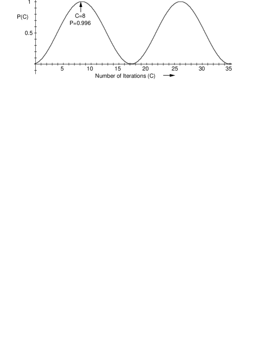
Figure 2: Probability for Grover search with $N=128$.

It is interesting to note that $P(C,N)$ is periodic in $C$. This can be seen clearly in Fig. 2 which graphs $P(C,N)$ against $C$ for $N=128$. Here, an optimum probability of success is reached after eight iterations, where $P(8,128)=0.996$. After eight iterations, the probability starts to decrease again. The reason for the decrease is that, after eight iterations, the average immediately after the inversion about the origin operation goes below zero.

We wish to determine the optimum number of iterations for a given $N$. $P$ reaches a maximum (and a minimum) for a given $N$ when:

$$\frac{d}{dx}P(x,N) = 0.$$

It is easy to show that the first maximum for a given $N$ is reached at

$$\frac{\pi}{4.\theta_{N}}-\frac{1}{2} \hbox{where}~{}\theta_{N}~{}=~{}\arcsin\frac{1}{\sqrt{N}}.$$

We call this $H(N)$. Thus the number of iterations in the Grover algorithm for a search space of size $N$ should be the closest whole number to $H(N)$. In Fig. 3, we graph $H(N)$ and indicate that it is ${\cal O}(\sqrt{N})$.

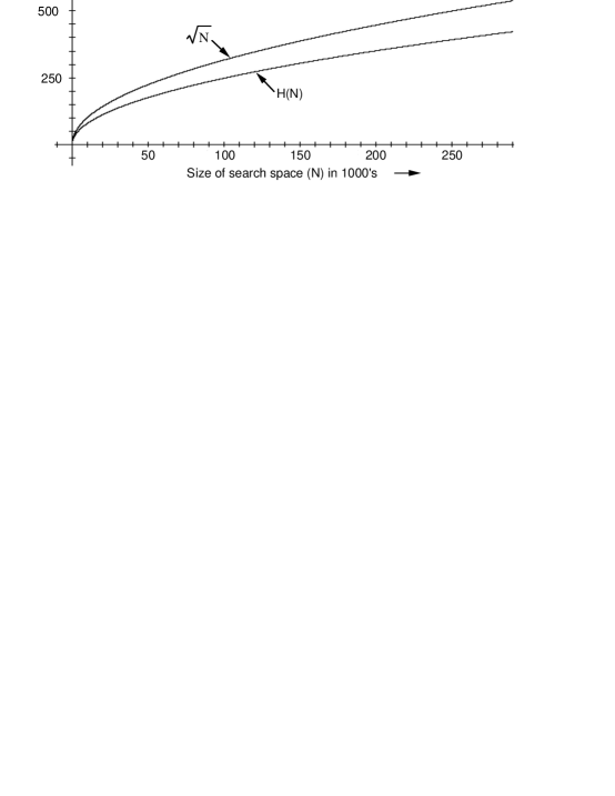
Figure 3: Optimum number of iterations versus search space size.

7 Conclusions

We have shown how Grover’s search algorithm may be represented in the programming notation of the probabilistic wp-calculus. Any quantum computation consists of unitary transformations and probabilistic measurement and these can be modelled in this notation. Thus any quantum algorithm may be modelled in the notation. We believe that this language provides a more rigorous and elegant means of describing quantum algorithms than is normally used in the literature.

We have also shown how the rules of the probabilistic wp-calculus may be used to derive a recursive formula for the probability that Grover’s algorithm finds the required solution. Using standard mathematical techniques, we were then able to then find a closed form for this probability which corresponds to the formula presented in [Boyer et al., 1998]. The wp-calculus provides a clear and systematic means of stating the required outcome and of deriving the probability of achieving it. Of course, it does not provide everything for free as we still had to use intelligence in recognising the recurring structure and in finding a closed form.

In the case of Grover, we were able to derive an exact probability for success because the algorithm iterates a fixed number of times. Some algorithms iterate until some condition is met rather a fixed number of times. One such example is a generalisation of Grover’s presented in [Boyer et al., 1998] which deals with the situation where there are an unknown number of values $x$ satisfying $f(x)=1$. In a case like this, we need to find the expected number of iterations rather than the probability of success. For future work, we intend to look at how these cases may be reasoned about using the probabilistic wp-calculus.

Appendix A Deriving a Closed Form

We outline the derivation of the closed form expression for the probability of success of Grover’s algorithm. The probability $P(C,N)$ is expressed in terms of the series $A_{i}$ and $B_{i}$, which in turn are defined by the recurrence equations (14) and (15). To find a closed form for these recurrences we first compute the generating functions for $A_{i}$ and $B_{i}$ using basic techniques [Knuth, 1973, Sect. 1.2.9]:

$$A_{i}~{}=~{}\frac{2Ni}{N+2(2-N)i+Ni^{2}} B_{i}~{}=~{}\frac{N-Ni}{N+2(2-N)i+Ni^{2}}.$$

Computing the probability involves the sum $A_{i}+B_{i}$ and it seems reasonable to examine the Taylor series expansion of the sum of the two generating functions. Assume that $z$ is such that the Taylor series expansion of $A_{z}+B_{z}$ converges:

$$A_{z}+B_{z}$$

$$= \frac{N+Nz}{N+2(2-N)z+Nz^{2}}$$

$$=$$ Taylor expansion

$$1+\frac{3N-4}{N}z+\frac{5N^{2}-20N+16}{N^{2}}z^{2}+\frac{7N^{3}-56N^{2}+112N-64}{N^{3}}z^{3}+\cdots.$$

We now observe that there is a strong similarity between the coefficients and powers of $N$ in the enumerators above and the coefficients and powers of $\sin(\theta)$ in the multiple angle formula for $\sin(n\theta)$:

$$\begin{array}[]{*{3}{@{~}l}}{}\lx@intercol\sin(1\theta)\hfil~{}&=\hfil~{}&1\sin(\theta)\\ {}\lx@intercol\sin(3\theta)\hfil~{}&=\hfil~{}&3\sin(\theta)-4\sin^{3}(\theta)\\ {}\lx@intercol\sin(5\theta)\hfil~{}&=\hfil~{}&5\sin(\theta)-20\sin^{3}(\theta)+16\sin^{5}(\theta)\\ {}\lx@intercol\sin(7\theta)\hfil~{}&=\hfil~{}&7\sin(\theta)-56\sin^{3}(\theta)+112\sin^{5}(\theta)-64\sin^{7}(\theta).\end{array}$$

This similarity suggests that we express $N$ in the form $\sin^{-2}(\theta)$ since, for example,

$$\frac{5N^{2}-20N+16}{N^{2}}[N/\sin^{-2}(\theta)] = 5-20\sin^{2}(\theta_{N})+16\sin^{4}(\theta_{N}).$$

We write $\theta$ as $\theta_{N}$ and choose it so that $\sin^{-2}(\theta_{N})=N$, i.e., $\theta_{N}=\arcsin\frac{1}{\sqrt{N}}$.

Rewriting $N$ as $\sin^{-2}(\theta_{N})$ in $A_{z}+B_{z}$ and re-calculating the Taylor series expansion gives:

$$A_{z}+B_{z} = \sum_{i=0}^{\infty}\left(1+2\sum_{j=1}^{i}\cos(2j\theta_{N})\right)z^{i}.$$

Since the Taylor series expansion has the form

$$A_{z}+B_{z} = \sum_{i=0}^{\infty}\left(A_{i}+B_{i}\right)z^{i},$$

we conclude that

$$A_{i}+B_{i} = 1+2\sum_{j=1}^{i}\cos(2j\theta_{N}).$$

The probability of success $P(C,N)$ is $|\!|~{}A_{C}+B_{C}~{}|\!|^{2}/N$. However, it is easy to see from equations (14) and (15) that for any positive naturals $C,N$, $A_{C}+B_{C}$ is real and not complex so that $|\!|~{}A_{C}+B_{C}~{}|\!|^{2}=(A_{C}+B_{C})^{2}$. We then obtain a closed form for the probability:

$$P(N,C) = |\!|~{}A_{C}+B_{C}~{}|\!|^{2}/N$$

$$= (A_{C}+B_{C})^{2}/N$$

$$= \left(1+2\sum_{j=1}^{C}\cos(2j\theta_{N})\right)^{2}/N$$

$$= \sin^{2}((2C+1)\theta_{N}).$$

References

- [Benioff, 1980] Benioff, P. (1980). The computer as a physical system: a microscopic quantum mechanical Hamiltonian model of computers as represented by Turing machines. Journal of Statistical Physics, 22:563–591.
- [Bernstein and Vazirani, 1993] Bernstein, E. and Vazirani, U. (1993). Quantum complexity theory. In 25th ACM Annual Symposium on Theory of Computing, pages 11–20.
- [Berthiaume, 1996] Berthiaume, A. (1996). Quantum computation. In Complexity Theory Retrospective II. Springer-Verlag. http://andre.cs.depaul.edu/Andre/publicat.htm.
- [Boyer et al., 1998] Boyer, M., Brassard, G., Høyer, P., and Tapp, A. (1998). Tight bounds on quantum searching. Fortschritte Der Physik, 46(4-5):493–505. Available from http://xxx.lanl.gov/abs/quant-ph/9605034.
- [Deutsch, 1985] Deutsch, D. (1985). Quantum theory, the Church-Turing principle and the universal quantum computer. In Royal Society London A 400, pages 96–117.
- [Dijkstra, 1976] Dijkstra, E. (1976). A Discipline of Programming. Prentice-Hall.
- [Ekert, 1994] Ekert, A. (1994). Quantum computation. In ICAP meeting. http://www.qubit.org/intros/comp/comp.html.
- [Grover, 1997] Grover, L. (1997). Quantum mechanics helps in searching for a needle in a haystack. Physical Review Letters, 79(2).
- [Knuth, 1973] Knuth, D. (1973). The Art of Computer Programming - Volume 1: Fundamental Algorithms. Addison-Wesley, Reading, Mass., second edition.
- [Morgan et al., 1996] Morgan, C., McIver, A., and Seidel, K. (1996). Probabilistic predicate transformers. ACM Transactions on Programming Languages and Systems, 18(3):325–353.