Tunneling Ionization Rates from Arbitrary Potential Wells

Abstract

We present a practical numerical technique for calculating tunneling ionization rates from arbitrary 1-D potential wells in the presence of a linear external potential by determining the widths of the resonances in the spectral density, $\rho(E)$, adiabatically connected to the field-free bound states. While this technique applies to more general external potentials, we focus on the ionization of electrons from atoms and molecules by DC electric fields, as this has an important and immediate impact on the understanding of the multiphoton ionization of molecules in strong laser fields.

While the behavior of atoms and molecules in strong laser fields has been studied for almost two decades, new phenomena continue to arise and a unified picture for either does not yet exist [1, 2, 3]. However, simple models for tunneling ionization [4, 5] have provided a crucial baseline for understanding atoms in strong fields, as deviations from this basic process in ion yields and electron energy spectra have pointed to new physics [1, 2, 6]. Conversely, the lack of a general tunneling model for molecules has seriously impeded the interpretation of molecular data which clearly hints at even richer phenomena [3, 7] than for atoms due to the extra degrees of freedom present in a molecule.

Ionization from even diatomic potential wells are more difficult to treat than atoms because the barrier to ionization can shift between the barrier separating the two wells and the outer barrier as a function of field strength and internuclear separation [8] (see Fig. 1). These situations are quite distinct and, indeed, this competition between barriers leads to interesting and complex behavior. Thus, it is critical for any tunneling ionization model to work for arbitrary potential wells so as to treat these different situations uniformly. Furthermore, a useful model for molecules in strong laser fields must be non-perturbative in both the rates and the Stark shifts. In this Letter we introduce a practical non-perturbative technique for computing tunneling ionization rates from an arbitrary 1-D potential well. After outlining the general method, we apply it to a single-well (‘atomic’) potential, yielding excellent agreement with existing theoretical analyses. Then we apply our method to a double-well (‘molecular’) potential, like that shown in Fig. 1, to illustrate the generality of the method and to show new features which arise due to the double-well structure. However, we emphasize that the method is exactly the same for any arbitrary shaped 1-D potential well.

The problem of determining ionization rates and Stark shifts non-perturbatively for an arbitrary potential in 1-D can be reduced to calculating the spectral density, $\rho(E)$. For potentials with strictly bound states $\rho(E)$ becomes a series of delta functions at the energy eigenvalues. Numerically integrating the Schrödinger equation (SE) determines these energies by finding the energy at which the wavefunction satisfies the given boundary conditions. This simple approach cannot be extended to the question of tunneling ionization because, by definition, the electron can escape to infinity. Given this fact, the electron’s state lies in the continuum; hence, all energies are allowed and simply integrating the SE at a particular energy provides little information, on its own. Rather, one must return to calculating $\rho(E)$ in general. In the presence of a linear potential, the delta functions in $\rho(E)$ for the bound states will evolve into Lorentzian-like resonances whose center positions reflect the Stark shift of the states and widths give their decay rates. As decay of the levels can only occur through ionization the width then directly gives the tunneling rate.

The limitation to 1-D potential wells may seem overly restrictive and requires some discussion. It is well known that ionization rates of atoms and molecules depend strongly on field strength [4]. For this reason ionization occurs overwhelmingly in the direction of the electric field, essentially reducing the problem to 1-D. For diatomic molecules, the ionization rate is much greater when the field is along the internuclear axis [9] and, again, reduces the problem to 1-D.

While a full discussion of $\rho(E)$ is rarely presented in standard books on quantum mechanics, a general approach exists for calculating $\rho(E)$, based on the Weyl-Titchmarsh-Kodaira (WTK) spectral theorem [10]. Remarkably, this approach is extremely well suited to numerical implementation. Essentially, the spectral theorem states that the “resolution of the identity” can be expressed as

$$\delta\left(x-y\right)=\sum_{i,j=1,2}\int^{\infty}_{-\infty}dE\,\phi_{i}\left(x,E\right)\phi_{j}\left(y,E\right)\rho_{ij}\left(E\right)$$ (1)

where $\phi_{1,2}(x,E)$ are two linearly independent eigenfunctions of the SE at energy $E$ and $\rho_{ij}(E)$ is the spectral density matrix. Before discussing how to calculate and interpret $\rho_{ij}(E)$, we must consider the question of normalization, as, in general, some of the states may lie in the continuum.

The usual concept of a finite square integral clearly cannot be used for the normalization of continuum wavefunctions. In the WTK approach, normalization is imposed locally by setting the Wronskian of the eigenfunctions equal to one which also ensures that $\phi_{1}$ and $\phi_{2}$ are linearly independent. Thus, we can choose the following initial conditions at any point $x=c\,$:

$$\begin{array}[]{cccc}\phi_{1}\left(c\right)=1,&\phi^{\prime}_{1}\left(c\right)=0,&\phi_{2}\left(c\right)=0,&\phi^{\prime}_{2}\left(c\right)=1.\end{array}$$ (2)

For convenience, we generally choose $x=0$. The complete functions $\phi_{i}(x)$ can now be found by numerically integrating the SE away from the origin using these initial conditions.

To construct the spectral density matrix $\rho_{ij}(E)$, we first find the linear combinations of $\phi_{1}$ and $\phi_{2}$,

$$\psi_{\pm}\left(x,\lambda\right)=\phi_{1}\left(x,\lambda\right)+m_{\pm}\left(\lambda\right)\phi_{2},$$ (3)

such that $\int_{-\infty}^{0}dx\,\left|\psi_{-}\right|^{2}$ and $\int_{0}^{\infty}dx\,\left|\psi_{+}\right|^{2}$ are both finite, where $\lambda=E+i\varepsilon$ and $\varepsilon\geq 0$. In other words, when the energy has a positive imaginary part, $\psi_{\pm}\left(x,\lambda\right)$ must decay sufficiently rapidly as $x\rightarrow\pm\infty$ to have a finite square integral on their respective half-line. This defines the functions $m_{\pm}\left(\lambda\right)$. The spectral density matrix is then [10]:

$$\rho_{ij}(E)={\frac{1}{\pi}}\lim_{\varepsilon\rightarrow 0}{\rm Im}{\frac{1}{m_{-}-m_{+}}}\left[\begin{array}[]{cc}1&{\frac{m_{-}+m_{+}}{2}}\\ {\frac{m_{-}+m_{+}}{2}}&m_{-}m_{+}\end{array}\right].$$ (4)

If the asymptotic wavefunctions of the external potential are known analytically, as is often the case, all that is needed to evaluate $m_{\pm}$ is the logarithmic derivative of the correctly decaying asymptotic wavefunctions of just the external potential, $\theta_{\pm}\left(x,\lambda\right)$: $f_{\pm}\left(x,\lambda\right)=\theta^{\prime}_{\pm}\left(x,\lambda\right)/\theta_{\pm}\left(x,\lambda\right)$ [11]. We can then solve for $m_{\pm}\left(\lambda\right)$:

$$m_{\pm}\left(\lambda\right)=-\left({\frac{\phi^{\prime}_{1}-f_{\pm}\phi_{1}}{\phi^{\prime}_{2}-f_{\pm}\phi_{2}}}\right).$$ (5)

Note that the overall normalization of the asymptotic wavefunctions is not important, as the logarithmic derivative is sufficient to determine $m_{\pm}\left(\lambda\right)$.

This entire procedure is very straightforward to implement numerically: starting with the boundary conditions in Eq. (2), $\phi_{1}$ and $\phi_{2}$ are found by integrating the SE away from the origin with a standard Runge-Kutta technique at a particular complex energy, $\lambda$. At the same time, $m_{\pm}$ are evaluated from Eq. (5). Ideally, one would integrate out to $\pm\infty$ to evaluate $m_{\pm}\left(\lambda\right)$ exactly. Since this is not possible numerically, we simply evaluate $m_{\pm}\left(\lambda\right)$ as a function of $x$ far enough from the local potential to where it converges to a constant value. At this point, $m_{\pm}\left(\lambda\right)$ have been determined as well as $\rho_{ij}(E)$ from Eq. (4).

To finish the problem, we must interpret the matrix in Eq. (4). The spectral density matrix, $\rho_{ij}(E)$, is positive definite [10] and, thus, its eigenvalues $\Lambda_{1}$ and $\Lambda_{2}$ are positive and represent scalar spectral density functions. In general, there are two functions because of the possibility of a two-fold degeneracy (corresponding, for example, to left and right moving solutions) on the whole line. However, in the case of a linear external potential (Fig. 1), one direction is inaccessible to a free particle and no degeneracy exists. In this case, either $\Lambda_{1}$ or $\Lambda_{2}$ will be on the order of $\varepsilon$ and is unimportant, leaving just one eigenvalue, resulting in a simple scalar spectral density. For problems on the half-line, $x\geq 0$, with a physical boundary condition at $x=0$, the spectral density matrix also reduces to a single spectral density function [10, 12]. Finally, we must consider taking the limit $\varepsilon\rightarrow 0$. Again, numerically, this is simple to specify: if the state can tunnel, it will have a “natural” width $\Gamma$ giving the tunneling rate and an “artificial” width determined by $\varepsilon$. One then decreases $\varepsilon$ until $\Gamma\gg\varepsilon$. We have noticed that the numerical results are surprisingly robust to changes in the various numerical parameters. We attribute this to the local specification of the normalization and initial conditions for the numerical integration and the ease in determining the $m_{\pm}$ values.

In order to test this method we considered tunneling ionization of a hydrogen atom by a DC electric field:

$$V(x)={\frac{1}{\sqrt{x^{2}+a^{2}}}}-Fx,$$ (6)

where $F$ is the field strength and $a=\sqrt{2}$ for a hydrogen atom. This 1-D form of the Coulomb potential [13] has proven to be an excellent model for strong field calculations because it preserves the long range $1/r$ dependence and has an infinite Rydberg-like series of bound states while removing the catastrophic singularity that occurs for 1-D. Furthermore, it has been used recently in direct calculations of the time-dependent Schrodinger equation for molecules [7]. Fig. 2 shows the spectral function at a moderate field strength. The first two low lying states in the Rydberg series can be seen, while the higher states have broadened and merged together. We stress that the blurring of the higher states is a real physical effect, due to the lowering of the potential barrier by the external field, and is not a limitation of the method. In a weaker field more of the excited states would be seen as well-defined peaks. Fig. 3 shows a typical unbound wavefunction at the peak of a resonance. At this point, most of the wavefunction is ”inside” the potential well, although it is still a continuum state. Fig. 4 shows the DC Stark shift as well as the first term in the second order perturbation theory expansion for the 1-D potential. Finally, Fig. 5 shows the tunneling ionization rate of the ground state as a function of field strength. In order to compare to a 3-D potential, we performed an angular average of the 1-D result:

$$\Gamma(F)={\frac{1}{2\pi}}\int d\Omega\,\Gamma\left(F\cos\theta\right).$$ (7)

As seen in Fig. 5, this averaged result agrees quite well with the standard 3-D static atomic tunneling model of ADK [4, 5]. However, the slight discrepancy at the higher intensity is intriguing. The ADK model depends on the ionization potential and the field strength, but does not take into account the DC Stark shift. While the shifts are small, ionization rates depend exponentially on ionization potential and the effect of the Stark shift on the ionization rate will increase with intensity. We recalculated the ADK rate using our calculation of the DC Stark shift, and, as seen in Fig. 5 the agreement between our angularly averaged model and the ADK result including the DC Stark shift is excellent.

The ’molecular’ or double-well potential has a much richer spectrum in an external field than an atom, and we cannot give a comprehensive treatment, here. However, as an example, we show, in Fig. 6, the effect of the separation of the double-well potential on ionization rates for both the ground and first excited states. The potential consists of two 1-D Coulomb potentials (Eq. 6) separated by a distance R, and the external field, as in Fig. 1. Using exactly the same method of calculating the spectral function and finding the widths of the peaks associated with the ground and first excited states, we find that the ionization rate is strongly dependent on the well separation, becoming greater at larger separations. Moreover, the qualitative shape of the ionization rate vs. intensity curve depends on the separation with apparently no saturation setting in for the excited state at the larger separation. In fact, these are just the conditions for electron localization and enhanced ionization predicted in Ref. [7]. These ionization rate curves can provide a framework to analyze experimental ion yield data from molecules.

In summary, we have described a practical numerical technique for calculating spectral density functions for arbitrary 1-D potentials on the whole line from which we can extract level shifts and tunneling rates. This will be of great value for interpreting data from atoms and molecules in strong laser fields.

We thank S. A. Fulling and W. P. Reinhardt for helpful discussions. We would like to acknowledge support from the NSF under grant PHY-9502935. G. N. G. was also supported through funding as a Cottrell Scholar of Research Corporation. K. J. B. was supported by the Research Experience for Undergraduates (REU) program of the NSF. G. D. acknowledges support from the DOE under grant DE-FG02-92ER40716.00.

Figure Captions

1. Molecular potential wells showing the importance of (a) the outer barrier and (b) the inner barrier.

2. Spectral density function for a model atom in an external field.

3. Potential in an external field with wavefunction on resonance.

4. Comparison of the 2nd order Stark shift calculation with perturbation theory, in atomic units.

5. Comparison of the angularly-averaged WTK tunneling rate model with a 3-D calculation (ADK) from Ref. [4].

6. Ionization rate of the ground and first excited state of a double-well potential for two different separations.

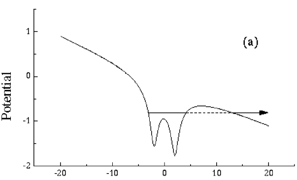
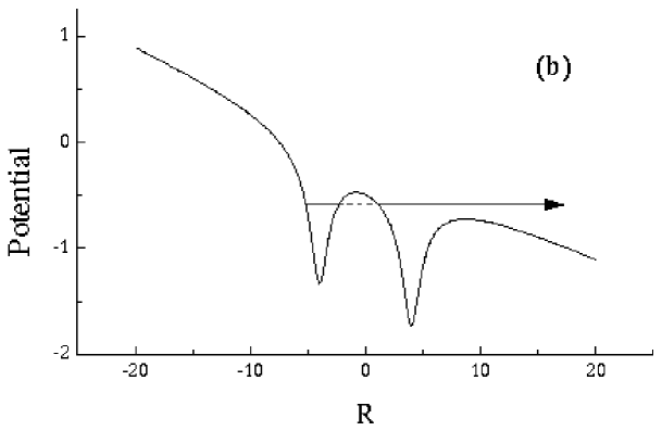
Figure 1: Molecular potential wells showing the importance of (a) the outer barrier and (b) the inner barrier.

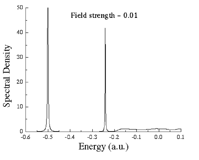
Figure 2: Spectral density function for a model atom in an external field.

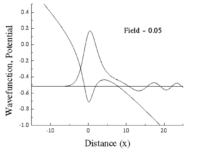
Figure 3: Potential in an external field with wavefunction on resonance.

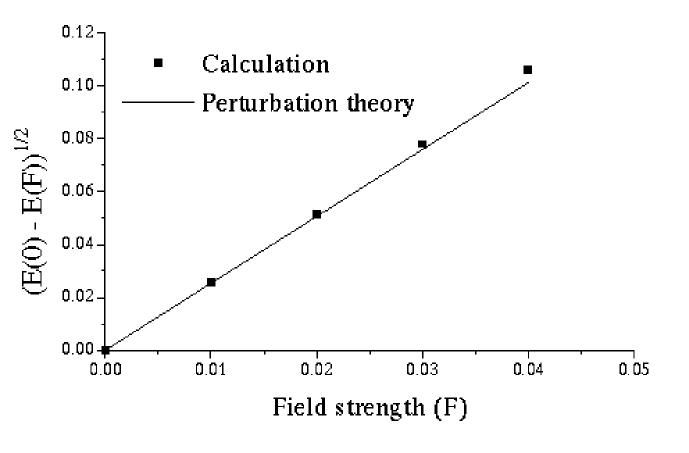
Figure 4: Comparison of the 2nd order Stark shift calculation with perturbation theory, in atomic units.

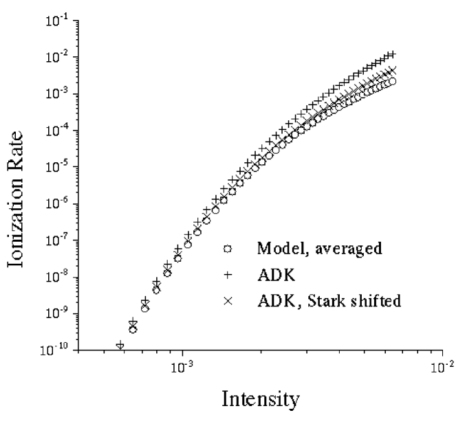
Figure 5: Comparison of the angularly-averaged WTK tunneling rate model with a 3-D calculation (ADK) from Ref. [4].

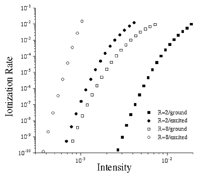
Figure 6: Ionization rate of the ground and first excited state of a double-well potential for two different separations.

References

- [1] B. Walker, B. Sheehy, L. F. DiMauro, P. Agostini, K. J. Schafer, and K. C. Kulander, Phys. Rev. Lett. 73, 1227 (1994).
- [2] P. Hansch, M. A. Walker, and L. D. Van Woerkom, Phys. Rev. A 55, R2535 (1997).
- [3] Such effects include: Non-sequential double ionization: A. Talebpour, S. Larochelle, and S. L. Chin, J. Phys. B 30, L245 (1997); Direct excitation: G. Gibson, T. S. Luk, A. McPherson, K. Boyer, and C. K. Rhodes, Phys. Rev. A 40, 2378 (1989); Stabilization: M. Schmidt, D. Normand, and C. Cornaggia, Phys. Rev. A 50, 5037 (1994); Dissociative recombination: A. Talebpour, C.-Y. Chien, and S. L. Chin, J. Phys. B 29, L677 (1996).
- [4] M. V. Ammosov, N. B. Delone, and V. P. Krainov, Sov. Phys. JETP 64, 1191 (1986).
- [5] P. B. Corkum, N. H. Burnett, and F. Brunel, Phys. Rev. Lett. 62, 1259 (1989).
- [6] P. B. Corkum, Phys. Rev. Lett. 71, 1994 (1993).
- [7] T. Seideman, M. Yu. Ivanov, and P. B. Corkum, Phys. Rev. Lett. 75, 2819 (1995).
- [8] K. Codling, L. J. Frashinski, and P. A. Hatherly, J. Phys. B, 22, L321 (1989).
- [9] P. Dietrich, D. T. Strickland, M. Laberge, Phys. Rev. A 47, 2305 (1993).
- [10] Eigenfunction Expansions Associated with Second-Order Differential Equations, Vols. I and II, E. C. Titchmarsh (Oxford University Press, Oxford, 1946); K. Kodaira, Am. J. Math 71, 921 (1949).
-
[11]
For a linear potential , the asymptotic
solutions are Airy functions, so
where and . - [12] For an interesting analytically solvable model on the half-line, see: C. E. Dean and S. A. Fulling, Am. J. Phys. 50, 540 (1982).
- [13] J. Javanainen, J. H. Eberly, and Q. Su, Phys. Rev. A 38, 3430 (1988).