Cavity-induced coherence effects in spontaneous emission from pre-Selection of polarization

Abstract

Spontaneous emission can create coherences in a multilevel atom having close lying levels, subject to the condition that the atomic dipole matrix elements are non-orthogonal. This condition is rarely met in atomic systems. We report the possibility of bypassing this condition and thereby creating coherences by letting the atom with orthogonal dipoles to interact with the vacuum of a pre-selected polarized cavity mode rather than the free space vacuum. We derive a master equation for the reduced density operator of a model four level atomic system, and obtain its analytical solution to describe the interference effects. We report the quantum beat structure in the populations.

PACS No. : 42.50.Ct, 42.50.Md

I Introduction

It is well known that the decay of close lying states in atomic systems can be quite different from that of the decay of an isolated state [1, 2, 3, 4, 5, 6, 7, 8, 9, 10]. This is because in the former case the transition amplitudes arising from each state can interfere with each other. This interference occurs provided the transition dipole matrix elements ($\vec{d}_{\alpha\beta}$) satisfy certain conditions[1]. To be more specific, let us consider two excited states $|i\rangle$ and $|j\rangle$ decaying to a common ground state $|g\rangle$. The condition for the interference between the two decay channels is

$$\vec{d}_{ig}.\vec{d}_{jg}^{*}\neq 0.$$ (1)

As a consequence of (1) the populations and coherences get coupled in the density matrix equation [1]:

$$\frac{\partial\rho_{ii}}{\partial t}=-2\gamma_{i}\rho_{ii}-(\Gamma\rho_{ji}+\Gamma^{*}\rho_{ij})~{}~{};$$ (2)

where $2\gamma_{i}$ is the decay rate of the level $|i\rangle$ and $\Gamma\propto\vec{d}_{ig}.\vec{d}_{jg}^{*}$. This coupling leads to some remarkable consequences as discussed in various references [1, 2, 3, 4, 5, 6, 7, 8, 9, 10, 11]. For example, such coupling leads to quantum beats [2, 3], phase dependent line shapes [4, 5, 8], quenching of spontaneous emission [6, 7], lasing without inversion [9], and interference in decay of nuclear levels [11] etc.

The question arises - what are the systems for which the condition (1) holds ? Consider for example the $j=1\rightarrow j=0$ transition in an atomic system. Let $|i\rangle$, $|j\rangle$ and $|g\rangle$ in the above example denote the states $|j=1,m=1\rangle$, $|j=1,m=-1\rangle$ and $|j=0,m=0\rangle$ respectively. In this case, simple algebra shows that

$$\langle 0,0|\vec{d}|1,1\rangle.\langle 1,-1|\vec{d}|0,0\rangle=-|d|^{2}(\hat{x}+i\hat{y}).(\hat{x}-i\hat{y})^{*}=0,$$ (3)

where $d$ is the reduced dipole matrix element. Thus, the interference between two decay channels $|1,1\rangle\rightarrow|0,0\rangle$ and $|1,-1\rangle\rightarrow|0,0\rangle$ will not occur. Xia et. al. [6] found states in Sodium dimer where the spin-orbit coupling makes the dipole matrix elements non-orthogonal as the states get mixed. Several proposals have been made [10] to obtain non-orthogonality. However, it is desirable to examine how the condition (1) can be bypassed. The condition (1) arises from the fact that spontaneous emission occurs in two orthogonal modes of polarization. Therefore if we pre-select the polarization mode, then we do not need the condition (1) for interference to occur. In order to pre-select the polarization, we consider the problem of spontaneous emission in a mode selective cavity. It is of course known that the cavity can provide a good way to manipulate the spontaneous emission from an excited atom [12].

FIG. 1.: A possible configuration for the pre-selection of polarizations of the cavity modes that can give rise to new coherences. The propagation vectors of the cavity modes $\vec{k}_{a},\vec{k}_{b}$ are along the Y-direction and cavity polarizations $\hat{\epsilon}_{a},\hat{\epsilon}_{b}$ are along the X-direction, with the quantization axis (Z-direction) fixed by the direction of the magnetic field $\vec{B}$.

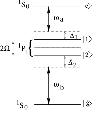
FIG. 2.: A four-level model scheme (say of ${}^{40}Ca$) with closely lying intermediate levels $|1\rangle\equiv|j=1,m=1\rangle$ and $|2\rangle\equiv|j=1,m=-1\rangle$. Here $\omega_{a}~{}(\omega_{b})$ is the frequency of the cavity field coupling $|e\rangle$ to $|1\rangle$ and $|2\rangle$ ($|1\rangle$ and $|2\rangle$ to the state $|g\rangle$). $2\Omega$ is the spacing between intermediate levels and the various detunings are defined by $\Delta_{j}=\omega_{ej}-\omega_{a}$, $\Delta_{j}^{\prime}=\omega_{jg}-\omega_{b}$.

In this paper, we demonstrate the possibility of restoring quantum interference effects in spontaneous emission of an excited atom inside a cavity with its modes selected suitably, and thus avoid the condition (1). A possible configuration is shown in Fig.1. In Section II, we describe the model atom which consists of two near-degenerate intermediate levels and orthogonal dipoles. The atom interacts with the cavity modes which are selected a priori. We consider the bad cavity limit and derive a master equation which shows evolution of quantum coherence between the degenerate or near degenerate levels. We obtain quantum beats in the populations of the intermediate states as well as the ground state. We present the solution of the master equation in Section III. We observe a decrease in the ground state population for some range of parameters. We compare these results obtained with and without interference terms. In Section IV, we show that, suitable selection of cavity polarization plays vital role in determining the occurrence of interference. Finally in Section V, we make some concluding remarks.

II Dynamics of a Four Level System in a Cavity

We consider a two-mode cavity containing a four-level atomic scheme with say, two near-degenerate Zeeman split magnetic sub-levels $|1\rangle\equiv|j=1,m=1\rangle$ and $|2\rangle\equiv|j=1,m=-1\rangle$ as its intermediate states (shown in Fig.2). The “$a$-mode” (“$b$-mode”) couples $|e\rangle\leftrightarrow|m\rangle$ ($|m\rangle\leftrightarrow|g\rangle$) transitions (for $m=\pm 1$). The scheme could be ${}^{40}Ca$-cascade, as shown by the symbols in the left hand side of the figure. The total Hamiltonian for the atomic system, and the cavity fields is

$$H=H_{A}+H_{F}+H_{AF},$$ (4)

where,

$$H_{A} = \hbar(\omega_{eg}A_{ee}+\omega_{1g}A_{11}+\omega_{2g}A_{22}),$$ (5)

$$H_{F} = \hbar(\omega_{a}a^{\dagger}a+\omega_{b}b^{\dagger}b),$$ (6)

$$H_{AF} = -\vec{d}.\vec{E}_{cav}$$ (7)

$$= -i\hbar\sum_{j=1}^{2}\left(G_{je}a^{\dagger}A_{je}+G_{gj}b^{\dagger}A_{gj}\right)+h.c.~{}.$$ (8)

Here state $|g\rangle$ is assumed to be the ground state; $\hbar\omega_{jg}=({\cal E}_{j}-{\cal E}_{g})$ (for $j\equiv e,1,2$) defines the energy of the atomic state $|j\rangle$ with respect to $|g\rangle$ and $A_{ij}=|i\rangle\langle j|$ are the atomic operators that denote populations (coherences) for $i=j$ ($i\neq j$). Further, $a,b$ ($a^{\dagger},b^{\dagger}$) are annihilation (creation) operators for the cavity field modes with frequencies $\omega_{a}$ and $\omega_{b}$ respectively. $E_{cav}$ is the quantized two mode cavity field. The atom-cavity mode coupling constants are given by

$$G_{je}=\left(\frac{2\pi\hbar\omega_{a}}{V}\right)^{1/2}\frac{\vec{d}_{je}.\hat{\epsilon}_{a}}{\hbar},G_{gj}=\left(\frac{2\pi\hbar\omega_{b}}{V}\right)^{1/2}\frac{\vec{d}_{gj}.\hat{\epsilon}_{b}}{\hbar},$$ (9)

with $V$ being the cavity volume and $\hat{\epsilon}_{a}$ and $\hat{\epsilon}_{b}$ being the polarizations of the cavity modes. We work in the interaction picture. The Hamiltonian in the interaction picture is given by

$$H_{I}(t) = e^{\frac{i}{\hbar}(H_{A}+H_{F})t}H_{AF}e^{-\frac{i}{\hbar}(H_{A}+H_{F})t}$$ (10)

$$= -i\hbar\sum_{j=1}^{2}\left(G_{je}a^{\dagger}A_{je}e^{-i\Delta_{j}t}+G_{gj}b^{\dagger}A_{gj}e^{-i\Delta_{j}^{\prime}t}\right)$$ (12)

$$+h.c.,~{}~{}j=1,2;$$

where, $\Delta_{j}=\omega_{ej}-\omega_{a}$ and $\Delta_{j}^{\prime}=\omega_{jg}-\omega_{b}$ are the detunings. The above Hamiltonian describes the reversible interactions between the atom and the cavity field. However we should also take into account the irreversible processes due to coupling of the cavity field with the outside world via cavity mirrors. We denote the leakage rates of the photons in the cavity modes by $\kappa_{a}$ and $\kappa_{b}$. At optical frequencies we can neglect the thermal photons. We further work in the bad cavity limit. The density matrix equation in the the interaction picture for the combined atom-field system contains two parts: (a) coherent evolution described by the Liouvillian $\Lambda$, and (b) the field relaxation part described by $\Lambda_{F}$ [13]

$$\frac{\partial\rho}{\partial t}=(\Lambda+\Lambda_{F})\rho,$$ (13)

where,

$$\Lambda\rho = -\frac{i}{\hbar}\left[H_{I}(t),\rho\right],$$ (14)

$$\Lambda_{F}\rho = -\kappa_{a}(a^{\dagger}a\rho-2a\rho a^{\dagger}+\rho a^{\dagger}a)$$ (16)

$$-\kappa_{b}(b^{\dagger}b\rho-2b\rho b^{\dagger}+\rho b^{\dagger}b).$$

To get useful information about the evolution of the atomic system, we derive the Master equation for the reduced atomic operator by approximately eliminating the cavity field using the standard projection operator techniques [1, 13]. In the following, we outline some of the important steps. We rewrite Eq.(8) as

$$\frac{\partial{\tilde{\rho}}}{\partial t}={\tilde{\Lambda}}(t){\tilde{\rho}}(t),$$ (17)

by transforming to a new frame with the transformations,

$${\tilde{\rho}}\equiv e^{-\Lambda_{F}t}\rho,~{}~{}{\tilde{\Lambda}}\equiv e^{-\Lambda_{F}t}\Lambda e^{\Lambda_{F}t}.$$ (18)

We define the projection operator to be ${\cal P}...\equiv\rho_{F}(0)Tr_{F}...$ and write Eq.(10) as,

$$\frac{\partial{\tilde{\rho}}}{\partial t}={\tilde{\Lambda}}{\cal P}{\tilde{\rho}}+{\tilde{\Lambda}}(1-{\cal P}){\tilde{\rho}}.$$ (19)

The assumptions that we make are (a) at $t=0$, $\rho(0)$ can be factorised into a product of atom and field density operators, (b) the photons emitted can not react back with the atom i.e., we use the Born approximation and (c) the Markoff approximation $G^{2}\kappa^{-1}\ll\kappa$ ($G$ refers to vacuum Rabi frequencies) which ensures that the system has a short memory. Using (10) and the above approximations and tracing over the field states Eq.(12) reduces to,

$$\frac{\partial{\rho_{a}}}{\partial t} = -\frac{1}{\hbar^{2}}$$ (20)

$$\times \lim_{t\rightarrow\infty}\int_{0}^{t}d\tau Tr_{F}\left[H_{I}(t),e^{\Lambda_{F}\tau}[H_{I}(t-\tau),\rho_{F}(0){\rho_{a}}]\right].$$ (21)

For convenience, $\tilde{\rho_{a}}$ is replaced by $\rho_{a}$ in (13) and in subsequent calculations.

The trace over the field operators inside the integral is calculated using the following relations. For arbitrary field operators $A$ and $B$, simple trace algebra and the definition of adjoints give

$$Tr_{F}\left[Ae^{\Lambda_{F}\tau}B\rho_{F}(0)\right]=\langle A(\tau)B\rangle,$$ (22)

$$Tr_{F}\left[Ae^{\Lambda_{F}\tau}\rho_{F}(0)B\right]=\langle BA(\tau)\rangle.$$ (23)

Further, the time correlations for the cavity fields in the absence of the interaction with the atom are known to be

$$\langle aa^{\dagger}(\tau)\rangle=\langle a(\tau)a^{\dagger}\rangle=e^{-\kappa_{a}\tau},$$ (24)

$$\langle bb^{\dagger}(\tau)\rangle=\langle b(\tau)b^{\dagger}\rangle=e^{-\kappa_{b}\tau},$$ (25)

with all other second order correlation functions being zero.

Substituting the complete Hamiltonian from Eq.(7) in (13) and using the relations (14), the trace inside the integral is expressed in terms of field correlations. Further using (15) and evaluating the integral in Eq.(13), we obtain the master equation for the atomic density operator

   

$$\frac{\partial{\rho}_{a}}{\partial t}= - i(\delta_{1}+\delta_{2})[A_{ee},{\rho}_{a}]-i[(\delta_{1}^{\prime}A_{11}+\delta_{2}^{\prime}A_{22}),\rho_{a}]$$ (26)

$$- \left\{\Gamma_{1}(A_{ee}{\rho}_{a}-2A_{11}{\rho}_{ee}+{\rho}_{a}A_{ee})+\Gamma_{1}^{\prime}(A_{11}{\rho}_{a}-2A_{gg}{\rho}_{11}+{\rho}_{a}A_{11})+1\rightarrow 2\right\}$$ (27)

$$+ \left\{2G_{1e}G_{2e}^{*}\frac{\kappa_{a}+i\Omega}{(\kappa_{a}+i\Delta_{2})(\kappa_{a}-i\Delta_{1})}A_{12}{\rho}_{ee}e^{2i\Omega t}+h.c.\right\}+\left\{2G_{g1}G_{g2}^{*}\frac{\kappa_{b}-i\Omega}{(\kappa_{b}+i\Delta_{2}^{\prime})(\kappa_{b}-i\Delta_{1}^{\prime})}A_{gg}{\rho}_{12}e^{-2i\Omega t}+h.c.\right\}$$ (28)

$$- \left\{G_{g1}^{*}G_{g2}e^{2i\Omega t}\left(\frac{1}{\kappa_{b}-i\Delta_{2}^{\prime}}A_{12}{\rho}_{a}+\frac{1}{\kappa_{b}+i\Delta_{1}^{\prime}}{\rho}_{a}A_{12}\right)+h.c.\right\}$$ (29)

where,

$$\Gamma_{j} = |G_{je}|^{2}\kappa_{a}/(\kappa_{a}^{2}+\Delta_{j}^{2}),~{}~{}\Gamma_{j}^{\prime}=|G_{gj}|^{2}\kappa_{b}/(\kappa_{b}^{2}+{\Delta_{j}^{\prime}}^{2}),~{}\Omega=(\omega_{1g}-\omega_{2g})/2,$$ (30)

$$\delta_{j} = |G_{je}|^{2}\Delta_{j}/(\kappa_{a}^{2}+\Delta_{j}^{2}),~{}~{}\delta_{j}^{\prime}=|G_{gj}|^{2}\Delta_{j}^{\prime}/(\kappa_{b}^{2}+{\Delta_{j}^{\prime}}^{2}),~{}~{}j=1,2~{}.$$ (31)

Here $\Gamma$ and $\Gamma^{\prime}$’s represent various decay constants from different levels and $\delta$ and $\delta^{\prime}$’s are the frequency shifts of atomic levels resulting from interaction with the vacuum field in a detuned cavity. This is the key equation of this paper and will be used in the subsequent analysis to study the coherence effects induced by the cavity.

To understand the meaning of various terms in the Master equation (26) we write the equations explicitly for the density matrix elements:

$$\frac{\partial\rho_{ee}}{\partial t}= - 2(\Gamma_{1}+\Gamma_{2})\rho_{ee},$$ (32)

$$\frac{\partial\rho_{11}}{\partial t}= - 2\Gamma_{1}^{\prime}\rho_{11}+2\Gamma_{1}\rho_{ee}-\eta~{}\frac{G_{g1}^{*}G_{g2}}{\kappa_{b}-i\Delta_{2}^{\prime}}\rho_{21}e^{2i\Omega t}-\eta~{}\frac{G_{g1}G_{g2}^{*}}{\kappa_{b}+i\Delta_{2}^{\prime}}\rho_{12}e^{-2i\Omega t},$$ (33)

$$\frac{\partial\rho_{12}}{\partial t}= - \left(\Gamma_{1}^{\prime}+\Gamma_{2}^{\prime}+i(\delta_{1}^{\prime}-\delta_{2}^{\prime})\right)\rho_{12}+2\eta~{}G_{1e}G_{2e}^{*}\frac{\kappa_{a}+i\Omega}{(\kappa_{a}+i\Delta_{2})(\kappa_{a}-i\Delta_{1})}\rho_{ee}e^{2i\Omega t}$$ (34)

$$- \eta~{}G_{g1}^{*}G_{g2}\left(\frac{\rho_{22}}{\kappa_{b}-i\Delta_{2}^{\prime}}+\frac{\rho_{11}}{\kappa_{b}+i\Delta_{1}^{\prime}}\right)e^{2i\Omega t},$$ (35)

$$\frac{\partial\rho_{gg}}{\partial t}= 2 \Gamma_{1}^{\prime}\rho_{11}+2\Gamma_{2}^{\prime}\rho_{22}+2\eta~{}G_{g1}G_{g2}^{*}\frac{\kappa_{b}-i\Omega}{(\kappa_{b}+i\Delta_{2}^{\prime})(\kappa_{b}-i\Delta_{1}^{\prime})}\rho_{12}e^{-2i\Omega t}+2\eta~{}G_{g1}^{*}G_{g2}\frac{\kappa_{b}+i\Omega}{(\kappa_{b}-i\Delta_{2}^{\prime})(\kappa_{b}+i\Delta_{1}^{\prime})}\rho_{21}e^{2i\Omega t}.$$ (36)

Equation for $\dot{\rho}_{22}$ is the same as for $\dot{\rho}_{11}$ with $1\leftrightarrow 2$ and $\Omega\rightarrow-\Omega$. Note the presence of oscillating components in (32). If $\Omega$ is large compared to damping constants $\Gamma$’s or detunings $\delta$’s, then these exponentials average out (shown explicitly in the discussion following Eq.(22)) leading to

$$\frac{\partial\rho_{ee}}{\partial t}= - 2(\Gamma_{1}+\Gamma_{2})\rho_{ee},$$ (37)

$$\frac{\partial\rho_{11}}{\partial t}= - 2\Gamma_{1}^{\prime}\rho_{11}+2\Gamma_{1}\rho_{ee},$$ (38)

$$\frac{\partial\rho_{12}}{\partial t}= - \left(\Gamma_{1}^{\prime}+\Gamma_{2}^{\prime}+i(\delta_{1}^{\prime}-\delta_{2}^{\prime})\right)\rho_{12},$$ (39)

$$\frac{\partial\rho_{gg}}{\partial t}= 2 \Gamma_{1}^{\prime}\rho_{11}+2\Gamma_{2}^{\prime}\rho_{22}.$$ (40)

These equations can be compared with the equations for emission in free space. Under the initial condition that the atom is in the state $|e\rangle$, equations (19) admit simple solutions:

$$\rho_{ee}(t) = \exp[{-2(\Gamma_{1}+\Gamma_{2})t}],$$ (41)

$$\rho_{11}(t) = \frac{\Gamma_{1}}{\Gamma_{1}+\Gamma_{2}-\Gamma_{1}^{\prime}}\left(\exp[{-2\Gamma_{1}^{\prime}t}]-\exp[{-2(\Gamma_{1}^{\prime}+\Gamma_{2}^{\prime})t}]\right),$$ (42)

$$\rho_{gg}(t) = 1-\rho_{ee}-\rho_{11}(t)-\rho_{22}(t),$$ (43)

and $\rho_{22}(t)$ is same as $\rho_{11}(t)$ with $1\leftrightarrow 2$.

For $\Omega$ comparable to $\Gamma$’s and $\Delta$’s, the exponential terms are important. The dynamical equations involve coupling of populations to coherences and vice-versa. Such couplings give rise to new coherence effects. Accordingly, let us introduce an interference parameter $\eta$ in Eq.(32), so that $\eta=1(=0)$ would refer to the presence (absence) of coherence effects.

III Quantum Coherences and Solution of The Master Equation

(a) Cavity Induced Intermediate State Coherence:

It is clear from Eq.(32) that, for $\eta=0$, the coherence between the intermediate levels is never established; i.e. $\rho_{ij}=0$ for all times. When $\eta$ is unity, there is a two-fold possibility for the coherence to evolve - (a) the second term in the equation for $\dot{\rho}_{12}$ causes evolution of coherence due to coupling of the states $|1\rangle$ and $|2\rangle$ to the excited state by the cavity vacuum field “$a$” and (b) the third term that arises from the coupling of $|1\rangle$ and $|2\rangle$ to the state $|g\rangle$ by the cavity vacuum field “$b$”. The resulting evolution of coherence is shown in Fig.3. For degenerate intermediate levels $|j\rangle$ $(j=1,2)$, and $\omega_{a}$ ($\omega_{b}$) in resonance with $|e\rangle\rightarrow|j\rangle$ ($|j\rangle\rightarrow|g\rangle$) transition, no such oscillation is seen - though coherence evolves.

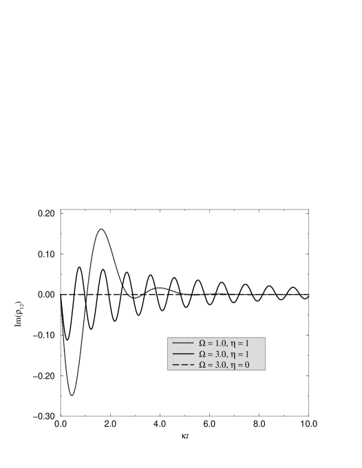
FIG. 3.: The time evolution of coherence between the intermediate states is plotted. All frequencies are scaled with $\kappa_{a}=\kappa_{b}=\kappa$. We choose $G_{je}\equiv G_{gj}=\kappa$, $\Delta_{1}^{\prime}=-\Delta_{2}^{\prime}=\Omega=-\Delta_{1}=\Delta_{2}$. For $\eta=0$, no coherence is produced, and for $\eta=1$, as $\Omega$ increases, the frequency of oscillation increases but the amplitude of coherence decreases.

(b) Cavity Induced Quantum Beats in Atomic Populations:

For $\eta=1$, the populations in Eq.(32) can be obtained analytically. For simplicity, assume that $\Gamma_{i}\equiv\Gamma_{i}^{\prime}\equiv\Gamma$, $G_{ie}\equiv G_{gi}\equiv G$, $\kappa_{a}\equiv\kappa_{b}=\kappa$ and the cavity field $\omega_{a}(\omega_{b})$ is tuned to the center of the two intermediate states and the excited (ground) state. Then, the solution of Eq.(32) is found to be

$$\rho_{ii}( t )=-\left(1+\frac{2|\alpha|^{2}}{\Gamma^{2}+f^{2}}\right)e^{-4\Gamma t}+\left(1+\frac{|\alpha|^{2}}{f^{2}}\right)e^{-2\Gamma t}$$ (44)

$$- \frac{2|\alpha|^{2}}{\Gamma^{2}+f^{2}}e^{-2\Gamma t}\left[\left(\frac{\Gamma^{2}}{f^{2}}-1\right)\cos(2ft)+\frac{2\Gamma}{f}\sin(2ft)\right],$$ (45)

$$\rho_{gg}( t )=1-\rho_{ee}(t)-2\rho_{ii}(t),i=1,2.$$ (46)

Here, the parameter $\alpha=GG^{*}/(\kappa+i\Omega)$ corresponds to the cross terms in Eq.(32). It can therefore be seen that for $|\alpha|=0$, Eq.(21) reduces to Eq.(20). The argument of the trigonometric functions in Eq.(44) gives the beat frequency

$$2f=2\left[(\delta^{\prime}+\Omega)^{2}-|\alpha|^{2}\right]^{1/2}.$$ (47)

The condition for the beats to occur is $(\delta^{\prime}+\Omega)^{2}>|\alpha|^{2}$. For various values of $\Omega$, we show the time dependence of $\rho_{ii}$ and $\rho_{gg}$ in Fig.4 assuming $|G|$ to be of the order of $\kappa$. If the intermediate levels are degenerate ($\Omega=0$), then $f$ is purely imaginary and therefore the trigonometric functions in Eq.(44) change to hyperbolic functions - ceasing the oscillations in the populations. Again, for $\Omega\ll\kappa$, $f$ is imaginary and hence there is no beating. However, for $\Omega\sim\kappa$, the beating in population is prominently seen. An increase in $\Omega$ leads to increase in the beat frequency. For $\Omega$ very large compared to $\kappa$, the beat frequency $2f\gg\kappa$ - leading to fast oscillations, the average of which leads to Eq.(20).

FIG. 4.: The time dependence of the populations in the ground state $\rho_{gg}$ (represented by I) and the intermediate states $\rho_{11}(=\rho_{22})$ (represented by II). The dashed lines represent $\eta=0$ where we see no oscillation. The solid lines represent $\eta=1$. The plots for various values of $\Omega$: (A) $\Omega=0$ - no beat structure is seen, (B) $\Omega=0.5\kappa$, (C) $\Omega=1.0\kappa$ and (D) $\Omega=3.0\kappa$ - where the population in the ground state decreases during $t\sim\kappa^{-1}$.

Further we note that for $\Omega(\sim 3\kappa)$, the ground state population decreases for a small time interval implying a population transfer to the intermediate levels. It should be borne in mind that, we work in the low-Q cavity limit where cavity vacuum is not strong enough to cause the vacuum field Rabi oscillation [14]. To interpret the decrease in population, we go back to Eq.(26). The 4th line of Eq.(26) suggests that the ground state population couples the intermediate state coherences via $G_{g1}G_{g2}^{*}$ (and $G_{g1}^{*}G_{g2}$); e.g., an emission followed by absorption of the same photon on a different transition. The corresponding transitions would correspond to $|1\rangle\rightarrow|g\rangle\rightarrow|2\rangle$ (and $|2\rangle\rightarrow|g\rangle\rightarrow|1\rangle$). The various transitions of $G_{ij}G_{il}^{*}$ type and various interference paths are illustrated in Fig.5. In particular from Fig.5(B), one understands the decrease in the ground state population.

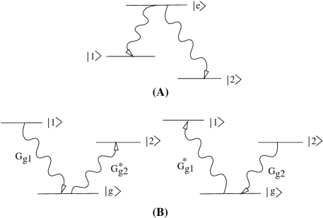
FIG. 5.: The various interference paths are shown by considering upper and lower transitions. (A) The upper $\Lambda$ like part: both transitions share a single reservoir of cavity vacuum - contributing to the coherence between the states $|1\rangle$ and $|2\rangle$. (B) The lower $V$ like part: to the lowest order interaction, photons emitted by $|1\rangle\leftrightarrow|g\rangle$ transition can be absorbed by $|g\rangle\leftrightarrow|2\rangle$ transition and vice versa - explaining the decrease in population of state $|g\rangle$.

IV Origin of Cavity Induced Coherences

We now examine the question - what leads to such coherences which otherwise do not occur. It is clear from Eq.(32) that, the coherence terms are related to matrix elements like

$$G_{g1}G_{g2}^{*}=\left(\frac{2\pi\omega_{b}}{\hbar V}\right)(\vec{d}_{g1}.\hat{\epsilon}_{b})(\vec{d}_{g2}^{*}.\hat{\epsilon}_{b}^{*}).$$ (48)

For the choosen geometry of Fig.1, Eq.(48) reduces to

$$G_{g1}G_{g2}^{*}=\left(\frac{2\pi\omega_{b}}{\hbar V}\right)(\vec{d}_{g1})_{x}(\vec{d}_{g2}^{*})_{x}.$$ (49)

The later is non-vanishing; as for $\sigma_{\pm}$ transitions, $\vec{d}_{g1}\equiv-|d|(\hat{x}+i\hat{y})$, $\vec{d}_{g2}=|d|(\hat{x}-i\hat{y})$. Note further that if polarization can not be pre-selected, then we have to sum Eq.(48) over the two possible polarization modes leading to

$$\sum_{pol}G_{g1}G_{g2}^{*} = \left(\frac{2\pi\omega_{b}}{\hbar V}\right)\sum_{pol}(\vec{d}_{g1}.\hat{\epsilon}_{b})(\vec{d}_{g2}^{*}.\hat{\epsilon}_{b}^{*})$$ (50)

$$= \left(\frac{2\pi\omega_{b}}{\hbar V}\right)(\vec{d}_{g1}.\vec{d}_{g2}^{*}).$$ (51)

Under these conditions the coherence term can survive only if the dipole matrix elements are non-orthogonal. It is thus clear that, in order to see the interferences or beats at $2\Omega$, one has to make a pre-selection of polarization so that coherence between $|1\rangle$ and $|2\rangle$ can be produced by spontaneous emission. Note that this is different from the usual quantum beat spectroscopy [15, 16] where coherence is produced by excitation with an external field of appropriate band width.

V Conclusions

In conclusion, we have shown: (a) how the pre-selection of polarization leads to certain types of interference effects which otherwise are missing unless the dipole matrix elements are non-orthogonal; (b) how the pre-selection of polarization can be achieved in a cavity. We demonstrate this in the context of a four level atomic system in a bimodal cavity in the limit of a bad cavity. We hope to consider the effect of the cavity quality on intermediate states coherences elsewhere.

REFERENCES

[1] G.S. Agarwal, “Quantum Statistical Theories
of Spontaneous Emission and their relation to other approaches”, Springer
Tracts in Modern Physics: Quantum Optics (Springer-Verlag, 1974), Sec.15.
[2]
D.A. Cardimona, M.G. Raymer, and C.R. Stroud Jr., J. Phys. B15,
55 (1982);
A. Imamoğlu, Phys. Rev. A40, 2835 (1989).
[4]
For studies of such coherence effects in the context of system see
J. Javanainen, Europhys. Lett. 17, 407 (1992);
S. Menon, and G.S. Agarwal, Phys. Rev. A57, 4014 (1998).
[5]
For studies on -systems, see [1];
P. Zhou, and S. Swain, Phys. Rev. Lett. 77, 3995 (1996);
ibid, 78, 832 (1997);
Phys. Rev. A56, 3011 (1997);
E. Paspalakis, S.Q. Gong, and P.L. Knight, Optics Commn. 152, 293 (1998).
[6]
H.R. Xia, C.Y. Ye, and S.Y. Zhu, Phys. Rev. Lett. 77, 1032 (1996);
G.S. Agarwal, Phys. Rev. A55, 2457 (1997).
[7]
S.Y. Zhu, R.C.F. Chan, and C.P. Lee, Phys. Rev. A52, 710 (1995);
S.Y. Zhu, and M.O. Scully, Phys. Rev. Lett. 76, 388 (1996);
H. Lee, P. Polynkin, M.O. Scully, and S.Y. Zhu, Phys. Rev. A55,
4454 (1997).
[8]
M.A.G. Martinez, P.R. Herczfeld, C. Samuels, L.M. Narducci, and C.H. Keitel,
Phys. Rev. A55, 4483 (1997);
E. Paspalakis, and P.L. Knight, Phys. Rev. Lett. 81, 293, (1998).
[9]
A. Imamoğlu, and S.E. Harris, Opt. Lett. 14, 1344 (1989);
S.E. Harris, Phys. Rev. Lett. 62, 1033 (1989).
[10]
We also note that several other methods have been suggested in
the literature to overcome the problem of orthogonal dipole matrix elements.
These include the application of d.c., r.f., or even optical fields depending
on the situation at hand. Here the non-orthogonality is obtained from
mixing of energy levels. The details can be found in
H. Schmidt, and A. Imamoğlu, Opt. Commn. 131, 333 (1996);
A. K. Patnaik, and G. S. Agarwal, J. Mod. Opt. 45, 2131 (1998);
E. Paspalakis, C. H. Keitel, and P. L. Knight, “Fluorescence control through
multiple interference mechanisms”, LANL preprint, quant-ph/9810072;
P. R. Berman, “An analysis of dynamical supression of spontaneous emission”,
LANL preprint, physics/9809005.
[11]
Coherence effects in the context of the decay of nuclear levels are discussed
in R. Coussement, M.V. Bergh, G. S’heeren, G. Neyens, and R. Nouwen,
Phys. Rev. Lett. 71, 1824 (1993).
[12]
For an excellent review and references on theories and experiments on cavity
induced changes of spontaneous emission, see S. Haroche, and D. Kleppner,
Phys. Today, January, 1989, p. 24.
For more recent reviews on this subject, see J.J. Childs, Kyungwon An.,
R.R. Dasari, and M.S. Feld in “Cavity Quantum
Electrodynamics”, ed. P.R. Berman (Academic Press, 1993), p. 325.
[13]
See the appendix in R.K. Bullough, Hyperfine Interaction 37, 71 (1987).
[14]
E.T. Jaynes, and F.W. Cummings, Proc. IEEE 51, 89 (1963);
G.S. Agarwal, J. Opt. Soc. Am. B2, 480 (1985);
H.I. Yoo and J.H. Eberly, Phys. Rep. 118, 239 (1985).
[15] Y.R. Shen, “The Principles of Non-linear Optics”,
(John Wiley & Sons, Inc., 1984), chap.13.
[16]
B. M. Garraway, and P. L. Knight [Phys. Rev. A54, 3592 (1996)] examined
the modifications in quantum beats of a -system, where the system is placed
in a cavity and is prepared in a coherent superposition of two excited
states.