Field purification in the intensity-dependent Jaynes-Cummings model

Abstract

We have found that, in the intensity-dependent Jaynes-Cummings model, a field initially prepared in a statistical mixture of two coherent states, $|\alpha\rangle$ and $|-\alpha\rangle$, evolves toward a pure state. We have also shown that an even-coherent state turns

periodically a into rotated odd-coherent state during the evolution.

I Introduction

The generation of nonclassical light and its interaction with matter are subjects of intense investigation in quantum optics. The increasing control of atoms and electromagnetic fields achieved nowadays has opened up exciting possibilities in this field. Details of the matter-field interaction have been investigated over the past thirty years, specially after the introduction of the Jaynes-Cummings model [1]. Despite of the simplicity of the model, it allows generalizations that may be applied to different circumstances and regimes [2]. One of these generalizations is the intensity dependent Jaynes-Cummings model, introduced by Buck and Sukumar [3]. Because of the commensurability of the Rabi frequencies which arises from such a coupling, this model presents absolutely periodic revivals, contrary to what happens in the ordinary Jaynes-Cummings model. Moreover, the state-vector representing the evolution of the system is periodic itself. This means that there will be periodic evolution for any expectation value. What has not been acknowledged is that this behaviour leads to such an enhancement of certain effects that would be otherwise difficult to notice within the realm of the original Jaynes-Cummings model. Because of this enhancement it is possible to have the generation of well-defined Schrödinger cat-like states during the evolution of the field in the intensity-dependent model, as it has been already discussed [4]. We would like to remark that the approach to a (almost) pure state at half of the revival time occurs in the ordinary Jaynes-Cummings model, as it is well known [5, 6], if we start with the field in a pure state. For an initial statistical mixture, however, only a tendency of purification occurs, instead of perfect purification.

In this paper we are going to be concerned with the dynamical change of field states, namely superpositions of coherent states. Of particular importance is the purification, i.e., the transformation of a statistical mixture of two coherent states, for instance, into a quantum superposition of coherent states. We know that normally processes such as the interaction of a field with its environment (leading to dissipation), and the resonant interaction of a field with atoms leads to important loss of coherence, which represents the destruction of the quantum properties of a field state. It is therefore important to look for ways of overcoming these very common demolition processes. Surprisingly enough we have found that the resonant intensity-dependent Jaynes Cummings model provides a possible purification procedure. This is connected to the intrinsic periodicity of the model, and it is easy to see how this reorganization occurs from the phase-space point of view. On the other hand, if we start with the field prepared in a (pure) even-coherent state, the model shows periodic revivals which occur at half of the time of the revivals for an initial coherent state [7]. Because the full periodicity of the model again, the atom returns to its initial state (the excited state, for instance) at the second revival. However, at the first revival the atom will invert its state, i.e., it will appear in the ground state. The atom-field disentanglement (with relatively high intensity fields) at that time guarantees that the field will be in a pure state, but due to the change in the atomic state, we expect that not to be the even-coherent state. In fact, the field at that first revival time becomes a rotated odd-coherent state, as we are going to show.

This paper is organized as follows: in Section II we present the solution of the model in terms of the density operator. We also show the evolution of the field purity. In Section III we discuss the purification procedure from the phase space point of view. In Section IV we analyze the evolution of fields initially prepared in pure states (even and odd coherent states).

II Density operator solution and the field purity

The Hamiltonian for the intensity-dependent Jaynes-Cummings model [3] under the RWA is given by

$$\hat{H}=\frac{\hbar\omega}{2}\sigma_{z}+\hbar\omega\left(\hat{a}^{\dagger}\hat{a}+\frac{1}{2}\right)+\hbar\lambda\left(\hat{R}\sigma_{+}+\sigma_{-}\hat{R}^{\dagger}\right),$$ (1)

where $\lambda$ is the usual atom-field coupling constant, $\sigma_{+}=\left|e\right\rangle\left\langle g\right|$ and $\sigma_{-}=\left|g\right\rangle\left\langle e\right|$ are the atomic creation and annihilation operators respectively and $\hat{R}=\hat{a}\left(\hat{a}^{\dagger}\hat{a}\right)^{1/2}$, $\hat{R}^{\dagger}=\left(\hat{a}^{\dagger}\hat{a}\right)^{1/2}\hat{a}^{\dagger}$. Because of the factor $\left(\hat{a}^{\dagger}\hat{a}\right)^{1/2}$, the interaction term is no longer linear in the field variables and represents an intensity-dependent coupling. Let us assume that the initial state of the system is the product state $\rho_{af}\left(0\right)=\rho_{a}\left(0\right)\otimes\rho_{f}\left(0\right)$, with the atom initially in the upper state, or $\rho_{a}\left(0\right)=|e\rangle\langle e|$. The solution for the time-dependent density operator is analogous to the one in the ordinary Jaynes-Cummings model [5, 8], so that the evolution operator in the (two-state) atomic basis is

$$U^{\dagger}(t)=\left[\begin{array}[]{cc}\hat{C}_{n+1}(t)&i\hat{S}_{n+1}(t)\hat{R}\\ i\hat{S}_{n}(t)\hat{R}^{\dagger}&\hat{C}_{n}(t)\end{array}\right],$$ (2)

where

$$\hat{C}_{n+1}=\cos\left(\lambda t\sqrt{\hat{R}\hat{R}^{\dagger}}\right),\ \ \ \ \ \ \hat{S}_{n+1}=\frac{\sin\left(\lambda t\sqrt{\hat{R}\hat{R}^{\dagger}}\right)}{\sqrt{\hat{R}\hat{R}^{\dagger}}},$$ (3)

and having the same expressions for $\hat{C}_{n}$ and $\hat{S}_{n}$ but with $\hat{R}^{\dagger}\hat{R}$ instead of $\hat{R}\hat{R}^{\dagger}$.

Therefore the time-evolved density operator will read

$$\hat{\rho}_{af}(t)=U(t)\hat{\rho}_{af}(0)U^{\dagger}(t)=\left[\begin{array}[]{cc}\hat{A}(t)\hat{\rho}_{f}(0)\hat{A}^{\dagger}(t)&\hat{A}(t)\hat{\rho}_{f}(0)\hat{B}^{\dagger}(t)\\ \hat{B}(t)\hat{\rho}_{f}(0)\hat{A}^{\dagger}(t)&\hat{B}(t)\hat{\rho}_{f}(0)\hat{B}^{\dagger}(t)\end{array}\right],$$ (4)

where $\hat{A}(t)=\hat{C}_{n+1}$ and $\hat{B}(t)=-i\hat{R}^{\dagger}\hat{S}_{n+1}$. After tracing over the atomic variables we obtain the reduced field density operator, or $\hat{\rho}_{f}(t)=Tr_{a}\left[\hat{\rho}_{af}(t)\right]$, which is given by

$$\hat{\rho}_{f}(t)=\hat{A}(t)\hat{\rho}_{f}(0)\hat{A}^{\dagger}(t)+\hat{B}(t)\hat{\rho}_{f}(0)\hat{B}^{\dagger}(t).$$ (5)

If the state of the initial field is an equally-weighted statistical mixture of two coherent states, or

$$\hat{\rho}_{f}(0)=\frac{1}{2}\left(|\alpha\rangle\langle\alpha|+|-\alpha\rangle\langle-\alpha|\right),$$ (6)

we have that

$$\hat{\rho}_{f}(t) = \frac{1}{2}\sum_{n,m}\frac{e^{-|\alpha|^{2}}}{\sqrt{m!}\sqrt{n!}}\alpha^{n}\alpha^{*}{}^{m}\left[1+(-1)^{n+m}\right]\Big{\{}\cos\left[\lambda t(n+1)\right]\cos\left[\lambda t(m+1)\right]|n\rangle\langle m|$$ (7)

$$+ \frac{\sqrt{n+1}}{\alpha}\sin\left[\lambda t(n+1)\right]\sin\left[\lambda t(m+1)\right]|n+1\rangle\langle m+1|\Big{\}}.$$ (8)

For the sake of simplicity we are going to consider the amplitude $\alpha$ as real. At half of the revival time ($t=\pi/2\lambda$), we note that, for $\overline{n}\gg 1$, each one of the terms in Eq. (8) become exactly equal to

$$\hat{A}(\pi/2\lambda)\hat{\rho}_{f}(0)\hat{A}^{\dagger}(\pi/2\lambda)=\hat{B}(\pi/2\lambda)\hat{\rho}_{f}(0)\hat{B}^{\dagger}(\pi/2\lambda)=\frac{1}{4}\left(|i\alpha\rangle-|-i\alpha\rangle\right)\left(\langle i\alpha|-\langle-i\alpha|\right),$$ (9)

so that he resulting field state will be equal to

$$\hat{\rho}_{f}(\pi/2\lambda)=\frac{1}{2}\left(|i\alpha\rangle-|-i\alpha\rangle\right)\left(\langle i\alpha|-\langle-i\alpha|\right),$$ (10)

which is a Schrödinger cat state rotated $\pi/2$ relatively to the initial states. This is an unexpected organization, because according to what it is normally found in the literature, the field returns to its initial state at most, which is a mixed one in this case.

In order to illustrate this peculiar behaviour, we can follow the evolution of the field purity, defined as

$$\zeta_{f}(t)=1-Tr_{f}\left[\widehat{\rho}_{f}^{2}(t)\right].$$ (11)

For an initial statistical mixture we have that

$$\zeta_{f}(t)=1-\left(T_{1;+}^{2}+T_{1;-}^{2}+T_{2;+}^{2}+T_{2;-}^{2}+2\left|T_{3;+}\right|^{2}+2\left|T_{3;-}\right|^{2}\right),$$ (12)

where

$$T_{1;\pm} = \sum_{n=0}^{\infty}P_{n}^{M}\left(\pm 1\right)^{n}C_{n+1}^{2},\ \ \ \ T_{2;\pm}=\sum_{n=0}^{\infty}P_{n}^{M}\left(\pm 1\right)^{n+1}\left(\frac{n}{\alpha^{2}}S_{n}^{2}\right),$$ (13)

$$T_{3;\pm} = \sum_{n=0}^{\infty}P_{n}^{M}\left(\pm 1\right)^{n+1}C_{n+1}\left(\frac{i\sqrt{n}}{\alpha}S_{n}\right),$$ (14)

and $P_{n}^{M}$ is the Poisson distribution $P_{n}^{M}=e^{-|\alpha|^{2}}|\alpha|^{2n}/n!$.

As we see in Fig. 1, because the field is initially in a mixed state, $\zeta(0)=0.5$. As time goes on we note a growth in $\zeta$, followed by a sudden decrease, almost down to zero at half of the revival time. Of course the total atom-field state can not have its purity diminished, which means that as the field becomes more pure the atomic state must be closer to a mixed state. Although this behaviour is not obvious, exists a neat explanation from the phase space point of view, as we are going to show below.

III Phase space approach

The representation of fields in phase space has been providing new insights of the Jaynes-Cummings field dynamics [7, 9, 10]. Perhaps the most convenient quasiprobability to be used in this kind of problem is the $Q$-function, defined as

$$Q(x,y;t)=\frac{1}{\pi}\langle\beta|\hat{\rho}_{f}(t)|\beta\rangle;\ \ \ \ \ \ \beta=x+iy.$$ (15)

For the specific initial state in Eq.(6), the corresponding $Q$-function will be given by

$$Q(x,y;t)=\frac{1}{2\pi}\left(\left|S_{1,+}\right|^{2}+\left|S_{1,-}\right|^{2}+\left|S_{2,+}\right|^{2}+\left|S_{2,-}\right|^{2}\right),$$ (16)

where the terms $S_{i,\pm}$ are

$$S_{1,\pm} = \left\langle\beta\right|\widehat{A}\left|\pm\alpha\right\rangle=\sum_{n=0}^{\infty}\frac{\exp\left[-\left(\left|\beta\right|^{2}+\alpha^{2}\right)/2\right]}{n!}\left(\beta^{*}\alpha\right)^{n}\left(\pm 1\right)^{n}C_{n+1}(t)$$ (17)

$$S_{2,\pm} = \left\langle\beta\right|\widehat{B}\left|\pm\alpha\right\rangle=\sum_{n=0}^{\infty}\frac{\exp\left[-\left(\left|\beta\right|^{2}+\alpha^{2}\right)/2\right]}{n!}\left(\beta^{*}\alpha\right)^{n}\left(\pm 1\right)^{n}\left[-\frac{i\beta^{*}S_{n+1}(t)}{\sqrt{n+1}}\right].$$ (18)

The $Q$-function shows a very clear picture of the field dynamics. It is already well-known that for an initial coherent state the collapse is associated to a split of the $Q$-function in two branches, and that at half of the revival time, when the field becomes very close to a pure state, the two branches are most far apart [7, 9]. In the case of an initial statistical mixture as in Eq.(6) (Fig. 2a), there will be counter-propagating branches (Fig. 2b), which “collide” at half of the revival time $(t=\pi/2\lambda)$, as it is illustrated in Fig. 2c. Because we start with an statistical mixture, this means that we have either one possibility or the other. It happens that exactly at half of the revival time, there is a complete overlap of the $Q$-functions representing both possibilities, and also at this time the field will be in a pure state for each one of them. Because of that overlap, there is only one possible state, which happens to be a pure state (Schrödinger cat).

IV Transition from even to odd-coherent states

It is worth analysing how would be the dynamics like if the initial field was a Schrödinger cat state, or

$$\hat{\rho}_{f}(0)=|\Phi\rangle\langle\Phi|;\ \ \ \ \ \ |\Phi\rangle={\cal N}^{1/2}\left(|\alpha\rangle+r|-\alpha\rangle\right),$$ (19)

being $r=\pm 1$ (even and odd-coherent state, respectively).

In this case, the time evolution will be such that

$$\hat{A}|\Phi\rangle = {\cal N}^{1/2}\sum_{n}\frac{e^{-|\alpha|^{2}/2}}{\sqrt{n!}}\alpha^{n}\left[[1+r(-1)^{n}\right]\cos\left[\lambda t(n+1)\right]|n\rangle,$$ (20)

$$\hat{B}|\Phi\rangle = {\cal N}^{1/2}\sum_{n}\frac{\sqrt{n}}{\alpha}\frac{e^{-|\alpha|^{2}/2}}{\sqrt{n!}}\alpha^{n}\left[[1-r(-1)^{n}\right]\sin\left[\lambda tn\right]|n\rangle.$$ (21)

The highly oscillating photon number distribution of the even (odd) coherent state,

$$P_{n}^{S}=\frac{\exp\left(-|\alpha|^{2}\right)|\alpha|^{2n}\left[1+r(-1)^{n}\right]^{2}}{n!\left[1+r^{2}+2r\exp\left(-2|\alpha|^{2}\right)\right]},$$ (22)

is nonzero only at even (odd) photon numbers, and therefore the first revival with this initial field occurs at half of the time ($t_{r}^{even}$) than for a coherent state ($t_{r}^{cohe}$) [7, 11], or

$$t_{r}^{even}\left[2\lambda t\left(\overline{n}+2\right)-2\lambda t\overline{n}\right]\approx 2\pi\ \ \ \ \ \ t_{r}^{even}=\frac{t_{r}^{cohe}}{2}=\frac{\pi}{2\lambda}.$$ (23)

The expressions in Eq.(19) become, at the revival time $t_{r}=\pi/2\lambda$ and in the limit of $\overline{n}\gg 1$,

$$\hat{A}|\Phi\rangle = \frac{i{\cal N}^{1/2}}{2}(1-r)\left(|i\alpha\rangle-|-i\alpha\rangle\right)$$ (24)

$$\hat{B}|\Phi\rangle = \frac{{\cal N}^{1/2}}{2i}(1+r)\left(|i\alpha\rangle-|-i\alpha\rangle\right).$$ (25)

We see that for an initial even coherent state $r=1$, the field state will become

$$|\psi\rangle=\frac{1}{\sqrt{2}}\left(|i\alpha\rangle-|-i\alpha\rangle\right),$$ (26)

i.e., a kind of odd-coherent state. However, at the second revival time $(t=\pi/\lambda)$, the field will return to its initial state (even-coherent state). There will be then a periodic change between odd and even coherent states of the field. Because those states differ by one photon, we expect the atom also to change state, i.e., to be found in the ground state when the field is in an odd-coherent state. This is confirmed if we follow the time-evolution of the (periodic) atomic population inversion $W(t)=<\sigma_{z}>$, that can be written in a closed form as follows

$$W(t) = \left[1+r^{2}+2r\exp\left(-2|\alpha|^{2}\right)\right]^{\left(-1/2\right)}\{\left(1+r^{2}\right)\exp[-2|\alpha|^{2}\sin^{2}(\lambda t)]\cos[|\alpha|^{2}\sin(2\lambda t)+2\lambda t]$$ (27)

$$+ 2r\exp[-2|\alpha|^{2}\cos{}^{2}(\lambda t)]\cos[|\alpha|^{2}\sin(2\lambda t)-2\lambda t]\}.$$ (28)

In Fig. 3 we have a plot of the atomic inversion as a function of $\lambda t$, where we see the flip from the upper to lower state occurring periodically. On the other hand, if the field is initially prepared in an odd-coherent state $(r=-1)$, there is never a transformation onto an even-coherent state; the field returning periodically to its initial state, as we easily see from Eq.(25).

V Conclusions

We have shown that the dynamics of the intensity-dependent Jaynes-Cummings model makes possible, for sufficient strong fields, to transform a statistical mixture of two coherent states into a Schrödinger cat state. This is a consequence of the intrinsic periodicity of the model, and can be readily explained from the phase-space point of view. We may ask why this behaviour has not been noticed by considering the field evolution in the ordinary Jaynes-Cummings model. The answer is that despite of the fact that the overlap (at half of the revival time) in phase space somehow occurs also in that case, the precise match between the clockwise and the counter-clockwise branches hardly happens. This is due to deformations of the branches as time goes on, and the less than perfect overlap means that we continue having two possible (mixed) states, although there is a tendency of purification. Nevertheless, perfect purification is not achieved in this case.

Regarding the transformation of the field from an even-coherent state to an odd-coherent state, the atom must change its state not only for energy conservation reasons, but also for parity conservation in the atom-field system. Both atom and field have well defined parity, and the change of atomic parity due to the transition from the excited state to the ground state is compensated by the change of the field from the even-coherent state to the (rotated $\pi/2$) odd-coherent state.

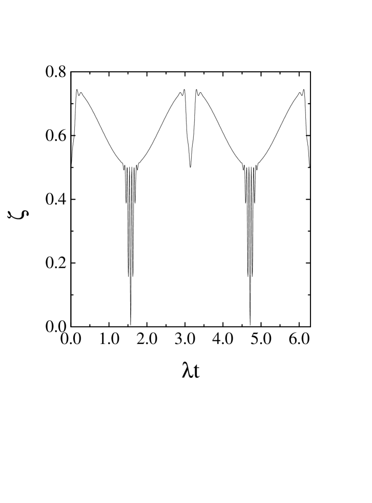
FIG. 1.: Field purity parameter $\zeta$ as a function of time for an initial statistical mixture of two coherent states $|\alpha\rangle$ and $|-\alpha\rangle$ ($\alpha=5$).

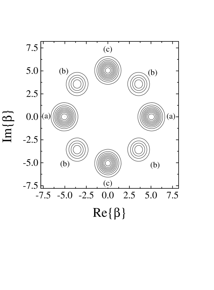
FIG. 2.: $Q$-function for an initial statistical mixture of two coherent states $|\alpha\rangle$ and $|-\alpha\rangle$ ($\alpha=5$), at different times, (a) $t=0$, (b) $t=\pi/4\lambda$ and (c) $t=\pi/2\lambda$.

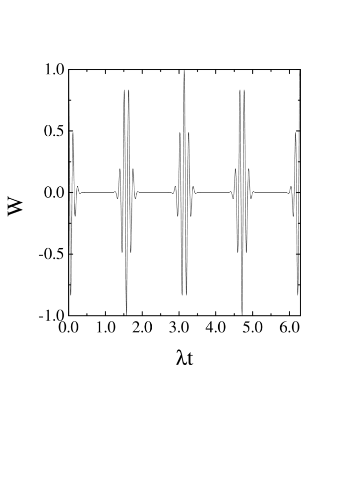
FIG. 3.: Atomic population inversion for the field initially prepared in an even-coherent state and the atom in the excited state with $\overline{n}=25$.

- [1] E.T. Jaynes and F.W.Cummings, IEEE 51 (1963) 89.
- [2] B.W. Shore and P.L. Knight, J. Mod. Opt. 40 (1993) 1195.
- [3] B. Buck and C.V. Sukumar, Phys. Lett. A 81 (1981) 132.
- [4] K. Zaheer and M.R.B. Wahiddin, J. Mod. Opt. 41 (1994) 150.
- [5] S.J.D. Phoenix and P.L. Knight, Ann. Phys. (N.Y.) 186 (1988) 381.
- [6] J. Gea-Banacloche, Phys. Rev. A 44 (1991) 5913.
- [7] A. Vidiella-Barranco, H. Moya-Cessa and V. Bǔzek, J. Mod. Opt. 39 (1992) 1441.
- [8] S. Stenholm, Phys. Rep. C 6 (1973) 1;
- [9] J. Eiselt and H. Risken, Phys. Rev A 43 (1991) 346.
- [10] K. Matsuo, Phys. Rev. A 50 649 (1994).
- [11] C.C. Gerry and E.E. Hach, Phys. Lett. A 179 (1993) 1.