Superluminal Signals: Causal Loop Paradoxes Revisited

Abstract

Recent results demonstrating superluminal group velocities and tachyonic dispersion relations reopen the question of superluminal signals and causal loop paradoxes. The sense in which superluminal signals are permitted is explained in terms of pulse reshaping, and the self-consistent behavior which prevents causal loop paradoxes is illustrated by an explicit example.

I Introduction

The idea of “tachyons”, i.e., particles that travel in the vacuum faster than light, has been the source of controversy for many years. Although special relativity does not strictly outlaw tachyons [1, 2, 3], the interaction of tachyons with ordinary matter does raise difficult questions. One of these is the possibility of violating the familiar relativistic prohibition of faster-than-light (superluminal) signals. A closely related concern is that any interaction of tachyons with ordinary matter would lead to logical inconsistencies through the formation of closed causal loops [4, 5, 6]. The participants in the ongoing debates are at liberty to hold their various views largely because of the complete absence of any experimental data. This unsatisfactory situation persists as far as true tachyons are concerned, but not with regard to “quasitachyons”, i.e., excitations in a material medium exhibiting tachyon-like behavior. Theoretical considerations have shown that superluminal and even negative group velocities are physically meaningful [7, 8, 9, 10], and that excitations with tachyonic dispersion relations exist [11, 12, 13, 14]. Superluminal group velocities have been experimentally observed for propagation through an absorbing medium [15], for microwave pulses[16, 17, 18] , and for light transmitted through a dielectric mirror [19, 20] . There has been a parallel theoretical controversy over the possibility of superluminal behavior in quantum tunneling of electrons and photons. Recent experiments using photons as the tunneling particles [19, 21, 22, 23] have confirmed Wigner’s early prediction that the time required for a particle to traverse a tunneling barrier of width $d$ can indeed be less than $d/c$.

The existence of superluminal group velocities and quasitachyons raises questions of the same general kind as those sparked by the previous speculations about tachyons. Is there any conflict with special relativity? Can these phenomena be used to send superluminal signals? What mechanism prevents logical contradictions through the formation of closed causal loops? In order to arrive at reasonably sharp and concise answers to these questions we will restrict the following discussion primarily to classical phenomena. The answer to the first question is straightforward. In all cases considered so far, the propagation of excitations in a medium is described by theories, e.g., Maxwell’s equations, which are consistent with special relativity; therefore, the predictions cannot violate special relativity. The remaining questions require somewhat more discussion. Superluminal signaling will be examined in Sec. II, in the context of choosing an appropriate definition of signal propagation speed. In Sec. III we investigate the issue of causality paradoxes in a somewhat simpler context. Finally the lessons drawn from these considerations will be discussed in Sec. IV.

II Superluminal signals

A common, if loosely worded, statement of an important consequence of special relativity is:“No signal can travel faster than light.” The more sweeping statement,“Nothing can travel faster than light.”, is contradicted by the familiar example of the spot of light thrown on a sufficiently distant screen by a rotating beacon [24]. The apparent velocity of the spot of light can exceed $c$, but this does not contradict special relativity since there is no causal relation between successive appearances of the spot. Any discussion of the first statement requires a definition of what is meant by a “signal” and what is meant by “signal velocity”. For our purposes it is sufficient to define a signal as the emission of a well defined pulse, e.g., of electromagnetic radiation, at one point and the detection of the same pulse at another point.

The classic analysis of Sommerfeld and Brillouin [25] identified five different velocities associated with a finite-bandwidth pulse of electromagnetic radiation propagating in a linear dispersive medium. We will consider here only the “front velocity”, the velocity of the “front”, i.e., the boundary separating the region in which the field vanishes identically from the region in which the field assumes nonzero values, and the “group velocity”, which describes the overall motion of the pulse envelope. It is worth noting that the definition of the front does not require a jump discontinuity at the leading edge of the pulse. Discontinuities of this kind are convenient idealizations suggested by the difficulty of following the behavior of the pulse at very short time scales, but they can always be replaced by smooth behavior. An envelope function which is sufficiently smooth at the front, e.g., the function and its first derivative vanish there, will have a finite bandwidth in the precise sense that the rms dispersion of the frequency, calculated from the power spectrum, will be finite. This definition of bandwidth is the one used in the uncertainty relation. The existence of the front has an important consequence which is best described in the simple example of one-dimensional propagation. If the incident wave arrives at $x=\mathrm{0}$ at $t=\mathrm{0}$ and the envelope, $u\left({\mathrm{x},t}\right)$, satisfies $u\left({\mathrm{0},t}\right)=\mathrm{0}$ for $t<\mathrm{0}$, then physically plausible assumptions for the behavior of the medium guarantee that the front propagates precisely at $c$, the velocity of light in vacuo[26]. On the other hand, the group velocity can take on any value. Indeed it has been shown that “abnormal” (either superluminal or negative) group velocities are required by the Kramers-Kronig relation for some range of carrier frequencies away from a gain line or within an absorption line[9].

The principle of relativistic causality states that a source cannot cause any effects outside its forward light cone. Since the front of a pulse emitted by the source traces out the light cone, this means that no detection can occur before the front arrives at the detector. A general signal will be a linear superposition of the elementary signals described above. The simplest model of this general behavior is that the pulse envelope $u\left({\mathrm{x},t}\right)$ is sectionally analytic in $t$, i.e., the front is a point of nonanalyticity separating two regions in which the pulse envelope has different analytic forms. The values of the pulse envelope on any finite segment in the interior of a domain of analyticity determine, by the uniqueness theorem for analytic functions, the pulse envelope up to the next point of nonanalyticity. It is therefore tempting to associate the arrival of new data with the points of nonanalyticity [22] in the pulse envelope. From this point of view, it is reasonable to identify the signal velocity with the front velocity. A happy consequence of this choice is that superluminal signals are uniformly forbidden, but this conceptual tidiness is purchased at a price in terms of experimental realism. By definition, the field vanishes at the front, and for smooth pulses will remain small for some time thereafter. Thus the front itself cannot be observed by a detector with finite detection threshold. Nevertheless, an operational definition of the front velocity can be given in terms of a limiting procedure in which identical pulses are detected by a sequence of detectors, ${D}_{n}$ , with decreasing thresholds ${S}_{n}$ . Let the pulse be initiated at $t=\mathrm{0}$ and denote by ${t}_{n}$ the time of first detection by ${D}_{n}$ , then the effective signal velocity is ${v}_{n}=d/{t}_{n}$,where $d$ is the distance from the source to the detector. The front velocity would then be defined by extrapolating ${v}_{n}$ as ${S}_{n}\mathrm{\rightarrow}\mathit{\mathrm{missing}}0$. While physically and logically sound, this procedure is scarcely practical.

We now turn from consideration of a series of increasingly sensitive detectors to a single detector with threshold close to the expected peak strength of the signal, ${S}_{\mathrm{0}}\mathrm{\ }\approx\mathit{\left missing}|{{u}_{peak}}\right|$ . We also assume that the pulse is not strongly distorted during propagation. Under these circumstances the pulse envelope propagates rigidly with the group velocity ${v}_{g}$. This suggests identifying the signal velocity with the group velocity. This is an attractive choice from the experimental point of view, but this benefit also has a price. First note that the peak cannot overtake the front [25] and that the front travels with velocity $c$. This prompts the question. In what sense is the signal superluminal even if ${v}_{g}>c$? To answer this, consider an experiment in which the original signal is divided, e.g., by use of a beam splitter. One copy is sent through the vacuum and the other through a medium, and the firing times of identical detectors placed at the ends of the two paths, each of length d, are then recorded. The difference between the two times, the “group delay”, is given by

$${t}_{g}={\frac{d}{{v}_{g}}}-{\frac{d}{c}}~{}.$$ (1)

The group delay is positive for normal media ($\mathrm{0}\mathit{<}{v}_{g}<c$ ), and negative for abnormal media, (${v}_{g}>c$ or ${v}_{g}<0$). It is only in this sense that the abnormally propagated signal is superluminal. With these definitions it is then correct to say that special relativity does not prohibit superluminal signals. This is a fairly innocuous complication of the usual discussion, but there are more serious problems related to the robustness of the definition. For example, if a more sensitive detector were used the measured group delay could be significantly smaller than that given by (1). Indeed as the threshold of the detector approaches zero, the group delay would approach zero. In other words the signal velocity would approach the front velocity. The only simple way to remove this ambiguity would be to identify the arrival of the pulse with the arrival of the peak. This would seem to attribute an unwarranted fundamental significance to the peak.

III Causal loop paradoxes

Causal loop paradoxes are usually introduced by considering two observers, A and B, each equipped with transmitters and receivers for tachyons. At time ${t}_{A}$, A sends a tachyonic message to B who then sends a return message to A timed to arrive at ${t}_{A}^{\mathrm{{}^{\prime}}}<{t}_{A}$, where both times are measured in A’s restframe. The paradox occurs if the return message activates a mechanism which prevents A from sending the original message [4]. Our next task is to reexamine this issue in the context of the two definitions of signal velocity discussed above. No paradoxical behavior is possible if the signal velocity is identified with the front velocity, since the signal velocity then equals the velocity of light. When the signal velocity is equated to the group velocity, more discussion is needed, since negative group delays are possible.

The core of the tachyon paradox is the ability to send messages into the past. It is therefore sufficient to devise a situation in which messages can be sent to the past at a single point in space [5]. A concrete example can be constructed by using an electronic circuit, for which the light transit time across the system is negligible compared to all other time constants. Propagation effects are then irrelevant, and the system can be described by a function, $V\left({t}\right)$, which depends only on time. For these systems we can use the principle of elementary causality which states that the output signal depends only on past values of the input signal. We will assume that both the input and the output pulse have well defined peaks occurring at ${t}_{in}$ and ${t}_{out}$ respectively. The time difference ${t}_{g}={t}_{out}-{t}_{in}$ is called the group delay by analogy to (1). Analyzing the relation between input and output in this way is analogous to choosing the group velocity to represent the signal velocity in the propagative problem. We can attempt to create the paradox by designing a circuit with negative group delay, i.e., the output peak leaves the amplifier beforethe input peak has entered. A low frequency bandpass amplifier with this rather bizarre property has been experimentally demonstrated [27], and it will be used in the following discussion. To get a message from the future it is necessary to construct a feedback loop in which the output of the amplifier is used to modulate the input, as shown in Fig. 1. If the amplifier produces a negative group delay this arrangement could apparently be used to turn off the input prematurely, e.g., before the peak.

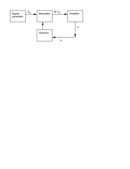
FIG. 1.: Feedback circuit: The modulator multiplies the input signal by $M(t)$ when the detector fires. The amplifier parameters are ${\mathrm{\omega}}_{r}=\mathrm{5}\mathit{\mathrm{missing}}1\mathit{H}z$ ,$\mathrm{\gamma}\mathit{=}\mathrm{1}\mathit{\mathrm{missing}}5\mathit{s}^{-\mathrm{1}\mathit{}}$ ,${T}_{\mathrm{0}}=\mathrm{2}\mathit{.}\mathrm{9}\mathit{\mathrm{missing}}4\mathit{m}s$

The Green’s function of the amplifier, i.e., the Fourier transform of the frequency-domain transfer function, is

$$G\left({t}\right)=\mathrm{\ }\delta\left({\mathit{t}}\right)\mathit{+}G\mathrm{{}^{\prime}}\left({\mathit{t}}\right)~{},$$ (2)

$$G\mathrm{{}^{\prime}}\left({\mathit{t}}\right)\mathit{\mathrm{missing}}\equiv\mathit{G}_{\mathrm{0}}\mathrm{\gamma}\mathit{\mathrm{missing}}\theta\left({\mathit{t}}\right)\mathit{e}^{-\mathrm{\ }\gamma\mathit{t}}\left[{\cos\left({{\mathrm{\omega}}_{r}t}\right)+{\frac{\mathrm{\gamma}}{{\omega}_{\mathit{r}}}}\sin\left({{\mathrm{\omega}}_{r}t}\right)}\right]~{},$$ (3)

where $\mathrm{\theta}\left({\mathit{t}}\right)$ is the step function, $\mathrm{\gamma}$ and ${\mathrm{\omega}}_{r}$ are respectively the damping rate and resonant frequency of the amplifier, and the dimensionless parameter ${G}_{\mathrm{0}}$ describes the overall amplification [27]. The presence of the step function in (3) imposes the retarded Green’s function and guarantees elementary causality. In the absence of feedback the output signal is

$${V}_{out}\left({t}\right)={V}_{in}\left({t}\right)+\int_{-\mathrm{\ }\infty}^{t}d\mathrm{\tau}\mathit{G}\mathrm{{}^{\prime}}\left({\mathit{t}-\mathrm{\ }\tau}\right)\mathit{V}_{in}\left({\mathrm{\tau}}\right)~{}.$$ (4)

A simple example of an input signal which has a continuous first derivative everywhere and vanishes outside a finite interval, is given by

$${V}_{in}\left({t}\right)={V}_{\mathrm{0}}\mathrm{\theta}\left({{\mathit{T}}_{\mathit{f}}\mathit{-}\left|{t}\right|}\right)\mathit{\cos}\left({{\mathrm{\omega}}_{c}t}\right){\cos}^{\mathrm{2}\mathit{}}\left({{\frac{\mathrm{\pi}\mathit{t}}{\mathrm{2}\mathit{T}_{f}}}}\right)~{}.$$ (5)

In the interior of the interval $\left({-{T}_{f},{T}_{f}}\right)$, this signal resembles a Gaussian pulse peaked at $t=\mathrm{0}$, and modulated at carrier frequency ${\mathrm{\omega}}_{c}$ . An example of negative group delay for this input is shown in Fig. 2.

FIG. 2.: $V_{out}(t)/V_{0}$(solid) and $V_{in}(t)/V_{0}$ (dashed) vs. time. Input pulse parameters ${\mathrm{\omega}}_{c}=\mathrm{0}$ , ${T}_{f}=\mathrm{4}\mathit{\mathrm{missing}}1\mathit{m}s$. This shows negative group delay, $t_{g}=-3.7ms$, for the parameters of Fig1.

In the feedback circuit the detector, with threshold set to ${S}_{\mathrm{0}}$, triggers the modulator which in turn multiplies the input voltage by a factor $M\left({t}\right)$. The input to the amplifier is then $M\left({t}\right){V}_{in}\left({t}\right)$, and the signal $V\left({t}\right)$ satisfies

$$V\left({t}\right) = M\left({t}\right){V}_{in}\left({t}\right)$$ (7)

$$+\int_{-\mathrm{\ }\infty}^{t}d\mathrm{\tau}\mathit{G}\mathrm{{}^{\prime}}\left({\mathit{t}-\mathrm{\ }\tau}\right)\mathit{M}\left({\mathrm{\tau}}\right){V}_{in}\left({\mathrm{\tau}}\right)~{}.$$

This seems to open the way for a variant of the time travel paradox in which the traveller journeys to the past and kills his grandfather before his own father is born. The analogous situation for the feedback circuit would be to employ the output peak to turn off the input before it has reached its peak. Fig. 2 shows that this seems to be possible. If there is a paradox, the integral equation (7) should fail to have a solution when the modulation function is chosen in this way. In an attempt to produce the paradoxical situation we choose the modulating function $M\left({t}\right)$ as follows. For any signal $V\left({t}\right)$ which rises smoothly from zero, define ${t}_{\mathrm{1}\mathit{}}$ and ${t}_{\mathrm{2}\mathit{}}$ as the first two times for which $\left|{V\left({t}\right)}\right|={S}_{\mathrm{0}}$. The first peak of the amplitude exceeding $S_{0}$ is guaranteed to lie between these two times, provided that the value of $S_{0}$ is below the absolute maximum value of the feedback signal. The modulating function is then chosen as

$$M\left({t}\right)=\mathrm{\ }\theta\left({{\mathit{t}}_{\mathit{\mathrm{missing}}2}\mathit{-}t}\right)~{}.$$ (8)

Thus the input is unmodulated until the peak of the feedback signal has passed and the detector again registers $S_{0}$. At this time the input is set to zero. The integral equation (7) for the signal is now

$$V\left({t}\right) = \mathrm{\theta}\left({{\mathit{t}}_{\mathit{\mathrm{missing}}2\mathit{}}\mathit{-}t}\right)\mathit{V}_{in}\left({t}\right)$$ (10)

$$+\int_{-\mathrm{\ }\infty}^{t}d\mathrm{\tau}\mathit{G}\mathrm{{}^{\prime}}\left({\mathit{t}-\mathrm{\ }\tau}\right)\mathit{\mathrm{missing}}\theta\left({{\mathit{t}}_{\mathit{\mathrm{missing}}2\mathit{}}\mathit{\mathrm{missing}}\tau}\right)\mathit{V}_{in}\left({\mathrm{\tau}}\right)~{}.$$

For times $t<{t}_{\mathrm{2}}$, the modulation function in both terms of (10) is unity, and comparison with (4) shows that $V\left({t}\right)={V}_{out}\left({t}\right)$ for $t<{t}_{\mathrm{2}}$ . Thus the time ${t}_{\mathrm{2}}$ is determined by the simple output function ${V}_{out}$, and the solution to (10) is

$${V}\left({t}\right) = \mathrm{\ }\theta\left({{\mathit{t}}_{\mathit{\mathrm{missing}}2\mathit{}}\mathit{-}t}\right)\mathit{V}_{out}\left({t}\right)+\mathrm{\theta}\left({\mathit{t}-{t}_{\mathrm{2}\mathit{}}}\right)\mathit{}$$ (12)

$$\times\int_{-\mathrm{\ }\infty}^{t}d\mathrm{\tau}\mathit{G}\mathrm{{}^{\prime}}\left({\mathit{t}-\mathrm{\tau}}\right)\mathit{\mathrm{missing}}\theta\left({{\mathit{t}}_{\mathit{\mathrm{missing}}2\mathit{}}\mathit{-}\mathrm{\tau}}\right)\mathit{V}_{in}\left({\mathrm{\tau}}\right)~{},$$

where $t_{2}$ is determined by $V_{out}$. A computer simulation of the solution, using the same parameters as in Fig. 1 , is plotted in Fig. 3. The self-consistent signal follows the amplifier output until the detector is triggered. This occurs after the output signal has reached its peak but before the input achieves its peak. The sudden termination of the input then sets off a damped oscillation. The existence of a self-consistent solution shows that there is no paradox; i.e., the theory does not suffer from internal contradictions. This feature is shared with previous resolutions of apparent paradoxes associated with tachyons [5, 6], or with the use of advanced Green’s functions in the Wheeler-Feynman radiation theory [28].

FIG. 3.: $V(t)/V_{0}$ and $V_{in}(t)/V_{0}$ vs time. Solution of the feedback equation (10) with $S_{0}=1.12V_{0}$. Input signal turned off 1.5 ms before its peak. Other parameters as in Fig. 1

IV Discussion and conclusions

In Sec. II we considered only two candidates for the signal velocity. While they may not be the only possibilities, the front and group velocities do seem to have the strongest a priori claims. Furthermore there is a form of complementarity between them. The front velocity is conceptually simple but operationally complex, and the group velocity is conceptually complex but operationally simple. Each alternative has strengths and weaknesses which we now discuss.

Identification of the front velocity as the signal velocity uniformly forbids the appearance of any superluminal signals, either in the vacuum or in a medium. This definition is Lorentz invariant, and it automatically excludes the possibility of any causal loop paradoxes. For a given distance $d$ between source and detector, the predicted arrival time $d/c$ represents the earliest possible time for detection. This interpretation is related to the most serious drawback of the definition, namely a detector with finite threshold cannot respond until some time $t>d/c$. Thus the arrival time $d/c$ can only be approximated by a limiting procedure such as that discussed in Sec. II. This objection is not fatal, since definitions of fundamental notions in terms of a limiting procedure are common, e.g., the definition of an electric field as the ratio of the force on a test charge to the charge as the charge approaches zero. An additional drawback is that the front-velocity definition mandates that all signals travel exactly at $c$, whether in the vacuum or in a medium. In particular this means that signals travel exactly at $c$ in normal dielectrics, not slower than $c$. This is not in accord with our usual usage and intuitions.

Identification of the group velocity with the signal velocity has the advantage of easy experimental realization, but there are also disadvantages. For example, one can imagine signals transmitted by pulses lacking a well defined group velocity, e.g., in the presence of strong group velocity dispersion. Furthermore, this definition actually requires the existence of superluminal signals, in the sense of negative group delays. In view of this, it is natural to wonder how superluminal signals can be consistent with special relativity. To begin, recall that special relativity is based on two postulates: (A) The laws of physics have the same form in all inertial frames. (B) The velocity of light in vacuo is independent of the velocity of the source. The first postulate is already present in Newtonian mechanics, so it is the second that leads to characteristically relativistic phenomena. Neither postulate says anything directly about the propagation of excitations in a material medium. The implications of special relativity for this question can only be found by using a theory of the medium, e.g., the macroscopic form of Maxwell’s equations, which is consistent with special relativity. In all such theories the response of the medium to the incident wave is described by retarded propagators, in accordance with both relativistic and elementary causality. With this in mind, superluminal propagation of electromagnetic fields can be understood as reshaping of the pulse envelope by interaction with the medium [10]. For propagation in a linear medium, it has long been known that the peak of the pulse can never overtake the front[25]. This conclusion holds for nonlinear media as well, e.g., superluminal propagation in a laser amplifier [29]. In all cases the pulse shape will become increasingly distorted as it asymptotically attempts to overtake the front.

The would-be paradoxical feedback circuit analyzed in Sec. III at first appears to present a puzzle. With the choice of parameters in Fig. 3, the peak of the feedback signal is used to turn off the input signal before it achieves its peak. This would seem to satisfy the requirements of the paradox, but the feedback problem does have a self-consistent solution. The apparent difficulty here stems from the natural assumption that the output peak is causally related to the input peak. This assumption has been criticized previously [24], and recent experimental results [27] , as well as the simulation results shown in Fig. 3, show it to be false. In order for event A to be the cause of event B, it must be that preventing A also prevents B. Both experiment and theory show that preventing the peak in the input does not prevent the peak in the output, therefore the peaks are not causally related. The peak in the output is however causally related to earlier parts of the input, since cutting off the input sufficiently early will prevent the output peak from appearing [30]. This shows that the analytic continuation of an initial part of the smooth pulse, discussed in Sec. II, is not just a theoretical artifact; the experimental apparatus actually performs the necessary extrapolation. However the apparatus cannot send a signal to any time prior to the initiation of the input signal. In other words, the output signal vanishes identically for $t<-{T}_{f}$; this is guaranteed by the use of retarded propagators.

The discussion so far has been carried out at the classical level, but there are general arguments suggesting that there will be no surprises at the quantum level. The relevant setting here is quantum field theory. In the Heisenberg picture the operator field equations have the same form as the classical field equations, so it is plausible that the solutions will be described by the same propagators. In particular, the electromagnetic field operators arising from an electric current localized in a small space-time region will be related to the source by the standard retarded propagator which vanishes outside the light cone. Indeed the solution to the point source problem involves only the retarded propagator even for models with tachyonic dispersion relations [31]. Explicit calculations for one such model display the same pulse reshaping features as the classical case [32]. A rigorous, general argument has been given by Eberhard and Ross [33], who show that if classical influences satisfy relativistic causality, then no signals outside the forward light cone will be observed in a fully quantal calculation. The essential point for their argument is the postulate that operators localized in space-like separated regions commute. This is used to show that actions performed in one region cannot change the probability distributions for measurements in a space-like separated region.

The first conclusion to be drawn from this discussion is that there is no completely compelling argument that would allow a choice between the proposed definitions of signal velocity. The front-velocity definition eliminates all superluminal signals and causality problems at a single stroke, but at the expense of an indirect operational definition. The group-velocity definition is operationally simple, but it provides a well defined sense in which superluminal signalling is allowed by relativity and by elementary causality, namely in those media allowing negative group delay. The description of negative group delay as superluminal propagation is, to some extent, a question of language. The values of the group delay, whether positive or negative, come from pulse reshaping effects. Thus one could speak of “group advance” for abnormal propagation and “group retardation” for normal propagation. The choice between “superluminal signal” and “group advance” is a matter of taste, but it should be kept in mind that the group delay is a measurable quantity and that negative values have been observed. Another point to consider is that before the work of Garrett and McCumber[7] the possibility of negative group delays would have been rejected as obviously forbidden by relativity. The second conclusion is that the superluminal propagation allowed by the group-velocity definition does not give rise to any causal loop paradoxes. The third conclusion is that no fundamental modifications in physics are needed to explain these phenomena. Finally the possibility of interesting applications of superluminal signals (in the sense of negative group delays) is an open question.

REFERENCES

- [1] O. M. Bilaniuk, V. K. Deshpande, and E. C. G. Sudarshan, Am. J. Phys. 30, 718 (1962).
- [2] S. Tanaka, Prog. Theor. Phys. 24, 171 (1960).
- [3] G. Feinberg, Phys. Rev. 159, 1089 (1967).
- [4] G. A. Benford, D. L. Book, and W. A. Newcomb, Phys. Rev. D 2, 263 (1970).
- [5] A. Peres and L. S. Schulman, Int. J. Theor. Phys. 6, 377 (1972).
- [6] L. S. Schulman, Am. J. Phys. 39, 481 (1971).
- [7] C. G. B. Garrett and D. E. McCumber, Phys. Rev. A 1, 305 (1969).
- [8] R. Y. Chiao, Phys. Rev. A 48, R34 (1993).
- [9] E. Bolda, R. Y. Chiao, and J. C. Garrison, Phys. Rev. A 48, 3890 (1993).
- [10] E. Bolda, J. C. Garrison, and R. Y. Chiao, Phys. Rev. A 49, 2938 (1994).
- [11] R. Y. Chiao, A. E. Kozhekin, and G. Kurizki, Phys. Rev. Lett. 77, 1254 (1996).
- [12] M. Blaauboer, A. E. Kozhekin, A. G. Kofman, et al., Opt. Commun. 148, 295 (1998).
- [13] M. Blaauboer, A. G. Kofman, A. E. Kozhekin, et al., Phys. Rev. A to appear (1998).
- [14] G. Kurizki, A. Kozhekin, and A. G. Kofman, preprint (1998).
- [15] S. Chu and S. Wong, Phys. Rev. Lett. 48, 738 (1982).
- [16] A. Enders and G. Nimtz, J. Phys. I 2, 1693 (1993).
- [17] G. Nimtz and W. Heitmann, Superluminal photonic tunneling and quantum electronics, in Progress in Quantum Electronics. 1997, p. 81.
- [18] A. Ranfagni, P. Fabeni, G. P. Pazzi, et al., Phys. Rev. E 48, 1453 (1993).
- [19] A. M. Steinberg, P. G. Kwiat, and R. Y. Chiao, Phys. Rev. Lett. 71, 708 (1993).
- [20] C. Spielmann, R. Szipocs, A. Stingl, et al., Phys. Rev. Lett. 73, 2308 (1994).
- [21] A. M. Steinberg and R. Y. Chiao, Phys. Rev. A 51, 3525 (1995).
- [22] R. Y. Chiao and A. M. Steinberg, Tunneling times and superluminality, in Progress in Optics, E. Wolf, Editor. 1997, Elsevier: New York. p. 347.
- [23] R. Y. Chiao and A. M. Steinberg, in Proceedings of the Nobel Symposium, edited by E. B. Karlsson and E. Braendas (Physica Scripta, Gimo, Sweden, 1997), Vol. 104.
- [24] R. Landauer, Nature (London) 365, 692 (1993).
- [25] L. Brillouin, Wave Propagation and Group Velocity (Academic Press, New York, 1960).
- [26] J. D. Jackson, Classical Electrodynamics (John Wiley and Sons, Inc., New York, 1975).
- [27] M. W. Mitchell and R. Y. Chiao, Phys. Let. A 230, 133 (1997).
- [28] J. A. Wheeler and R. P. Feynman, Rev. Mod. Phys. 21, 425 (1949).
- [29] A. Icsevgi and W. E. Lamb, Phys. Rev. 185, 517 (1969).
- [30] G. Diener, Phys. Let. A 223, 327 (1996).
- [31] Y. Aharonov, A. Komar, and L. Susskind, Phys. Rev. 182, 1400 (1969).
- [32] P. W. Milonni, K. Furuya, and R. Y. Chiao, preprint (1998).
- [33] P. H. Eberhard and R. R. Ross, Found. Phys. Lett. 2, 127 (1989).