Quantum observables associated with Einstein localisation

1 Introduction

Time and space are basic elements of our physical comprehension of the world. They are also among the physical quantities which are measured with the greatest accuracy. Yet their precise status raises questions in physical theory and different notions of time and space are used depending on the problem which is considered.

This idea is clearly emphasised by the following quotations from Newton’s Principia  [?]:

“Absolute, true, and mathematical time, of itself, and from its own nature, flows equably without relation to anything external, and by another name is called duration”

“Relative, apparent and common time, is some sensible and external measure of duration by the means of motion, which is commonly used instead of true time”

“Absolute space, in its own nature, without relation to anything external, remains always similar and immovable”

“Relative space is some movable dimension or measure of the absolute spaces; which our senses determine by its position to bodies; and which is commonly taken for immovable space”

These quotations show that theoretical physics has been built on at least two different notions of time and space from its very beginning. On one hand, time and space are defined as the mathematical parameters used to write down the equations of motion of theoretical physics. On the other hand, time and space are physical quantities which are obtained through measurements.

When he introduced relativistic conceptions of space-time, Einstein emphasised that true physical notions were that of observables. A physical time has to be associated with an event such as the tick of a clock or the click of a detector. He then demonstrated that time and space observables are relativistic observables. In particular, time and space observables are mixed under Lorentz frame transformations so that the notion of simultaneity is no longer absolute  [?].

Remote clocks have to be synchronised through the transfer of time references. A particularly important concept introduced by Einstein is that of clock synchronisation through the transfer of light pulses. This synchronisation procedure and the related localisation procedure which consists in the exchange of several time references between different observers  [?] are nowadays used for practical applications such as the Global Positioning System  [?] or the definition of reference systems  [?].

The previous arguments refer to classical theory of relativity but it should be obvious that time and space observables certainly belong to the quantum domain. The modern metrological definition of time and space has its roots in atomic physics and is hence based on quantum theory. The time delivered by an atomic clock is nothing but the phase of a quantum oscillator. Electromagnetic signals used in synchronisation or localisation procedures are quantum fields. As a consequence, any practical realisation of time has to meet quantum limitations at some level of accuracy  [?].

This discussion revives the basic idea contained in Newton’s quotations reproduced above, now in the context of physical theories of 20^th century. Physicists deal with two different notions of time and space. The equations of motion of classical physics, but also those of quantum field theory and of general relativity, are written in terms of coordinate parameters, i.e. classical numbers which map space-time. A basic assumption of general relativity is that this mapping is arbitrary. These classical coordinate parameters necessarily differ from time and space observables involved in any physical measurements. Space-time observables are relativistic observables which are mixed under frame transformations as well as quantum observables which have quantum fluctuations and cannot be represented as classical numbers.

In this context arises the particularly acute problem of ‘quantum time’. Since it is often argued that standard quantum formalism does not allow for time being treated as an operator  [?], the very status of time in quantum theory remains a matter of debate  [?]. The formalism does not provide a precisely stated energy-time Heisenberg inequality which should rely on a quantum commutation relation. Meanwhile, time has a different description from space which spoils the attempts to conciliate quantum definition of observables with relativistic behaviour under Lorentz transformations  [?]. These inconsistencies between quantum formalism and relativistic requirements are known to be knotty points in the attempts to include gravity in quantum theory  [?].

Einstein introduced the principle of relativity a few months after having proposed the hypothesis of light quanta  [?]. He incidentally noticed that energy and frequency of the electromagnetic field change in the same manner in a transformation from one inertial frame to another  [?]. This remark may be considered as the first demand for consistency between quantum and relativistic theories. Two years later, Einstein laid down the principle of equivalence of gravity and acceleration and predicted the existence of gravitational redshifts. He again noticed that energy and frequency change in the same manner under frame transformations  [?].

In modern quantum theory, the similarity of energy and frequency shifts has to be interpreted as an invariance property for particle number. This property is well known for Lorentz transformations but usually not admitted for transformations to accelerated frames. The latter are commonly represented by Rindler transformations  [?] which do not preserve the propagation equations of electromagnetic fields and result in a transformation of vacuum into a thermal bath  [?,?,?]. Since the concepts of particle number and vacuum play a central role in the interpretation of quantum field theory, this fact spoils the attempts to interpret the Einstein equivalence principle in the quantum domain  [?,?].

2 Outline

The basic idea underlying our approach is that relativistic effects can no longer be described by classical relativity. A new theoretical framework has to be built up where quantum and relativistic requirements are treated simultaneously and consistently. Our proposal for building up such a ‘quantum relativity’ is to import the conception of relativistic effects built on symmetries from classical theory into a quantum algebraic theory.

A basic property of relativistic observables is that they undergo shifts under frame transformations. These shifts are however perfectly compatible with invariance properties. In fact, they result from symmetries of the laws of physics in such a manner that the relations between observables have their form preserved under transformations. To be more precise, symmetries are described by algebraic techniques which ensure that relations between observables are universal, i.e. are independent of the specific frame in which they are written. Theoretical constraints associated with invariance are related to, but also distinct from, covariance constraints corresponding to the arbitrariness of coordinate mapping. A historical account of the relativistic approaches emphasising respectively invariance and covariance properties may be found in  [?].

To make the discussion more concrete, let us consider a synchronisation procedure where an emitter sends a light pulse to a remote receiver (see Figure 1).

Figure 1: Einstein synchronisation: two remote observers, each with a clock at his disposal, transfer a time reference by exchanging a light pulse.

The two observers respectively encode and retrieve a time information in the light pulse. In other words, they share a field observable which is easily identified in a classical context as the light-cone variable $u$ defined along the line of sight

$$t_{e}-\frac{x_{e}}{c}=u=t_{r}-\frac{x_{r}}{c}$$ (1)

$t_{e}$ and $t_{r}$ are the emission and reception times, as delivered to the emitter and receiver by their own clocks; $x_{e}$ and $x_{r}$ are the space coordinates of the emitter and receiver, as measured along the line of sight; $c$ is the velocity of light. Clearly, such a synchronisation relies on a symmetry of physics, the existence of a universal propagation velocity $c$. Meanwhile the time reference shared by the two observers is a quantity preserved by field propagation, namely the light-cone variable $u$.

The localisation of an event in space-time may then be operationally defined as the result of several time transfers corresponding to different propagation directions (see Figure 2).

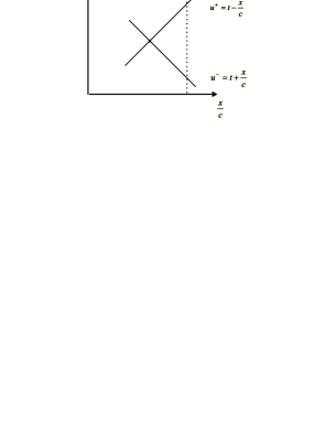
Figure 2: Einstein localisation represented on a space-time diagram: space and time correspond respectively to horizontal and vertical axis; light rays are indicated by straight lines making a $45^{\circ}$-angle with the axis; a motionless observer is represented by a vertical time-like trajectory; by operating two time transfers along two different directions, he is able to get positions in space and time of an event.

A motionless observer obtains the positions in time and space of an event by measuring two light-cone variables

$$t-\frac{x}{c}=u^{+} t+\frac{x}{c}=u^{-}$$

$$t=\frac{u^{-}+u^{+}}{2} \frac{x}{c}=\frac{u^{-}-u^{+}}{2}$$ (2)

It follows from the previous arguments that the relativistic notion of space-time is ultimately based upon the Poincaré symmetry of field propagation. These discussions look familiar since the invariance of Maxwell equations under Lorentz transformations played a prime role in Einstein’s introduction of classical relativity. They have been repeated here to prepare the reader to their quantum counterparts.

In quantum theory, the field observables can no longer be defined as classical numbers. Taking into account this essential difference, most preceding discussions are still relevant. In particular, the time references used in synchronisation and localisation procedures have to be observables preserved under propagation, that is also quantities built on the generators of the symmetries of field propagation. We will give below the definitions of synchronisation and localisation observables in terms of symmetry generators.

Symmetries also play a primary role in fundamental metrology. Translation symmetry allows one to transport metrological standards from one place to another. Lorentz symmetry permits one to use standards in different inertial frames and to derive a length unit from the time unit. The role played by dilatation is less often discussed although the invariance of Maxwell equations under dilatations has been known for a long time  [?]. Dilatations are naturally involved in comparisons of lengths or durations with different scales.

Meanwhile the metrological definition of units is more and more evolving towards the use of quantum standards. This is not only a result of technological progress but, more basically, of efforts to improve the universality of the definition of units. Dilatation symmetry plays a central role in this context as soon as dilatation is understood as a correlated change of time, space and mass scales which preserves the velocity of light and the Planck constant  [?,?,?]. A correlated variation of time and mass scales under dilatations is just the expression of the equivalence principle or, equivalently in a metrological context, of a consistent definition of units  [?].

These ideas may be applied to accelerated frames as soon as the latter are given a conformal representation. The interest of this representation relies on conformal invariance of Maxwell equations  [?,?]. Moreover, conformal coordinate transformations fit the motion of uniformly accelerated observers like Lorentz transformations fit the motion of inertial observers  [?]. Conformal invariance also means that propagation of electromagnetic fields is not sensitive to a conformal variation of the metric tensor, that is a change of space-time scale preserving the velocity of light  [?]. Hence, light propagates along straight lines while frequencies are preserved under propagation. Of course, redshifts are still present since clocks rates are affected by the conformal factor.

Conformal invariance can be rigorously established for quantum electromagnetic fields  [?]. Moreover, the definition of photon number is conformally invariant  [?]. The concept of photon and, in particular, the concept of vacuum  [?] are thus the same for inertial and uniformly accelerated observers which opens the way to an extension of ‘quantum relativity’ to accelerated frames  [?,?,?,?].

3 Clock synchronisation

We now address the problem of clock synchronisation performed with quantum fields. We focus our attention on quantum dispersions of energy density along the line of sight (see eq. (1)). We may therefore consider at this stage the simple theory of a scalar massless field propagating along a single direction in a two-dimensional (2d) space-time. The light pulse used as a time reference is schematically represented on Figure 3.

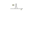
Figure 3: Dispersion along the line of sight of a pulse used as a time reference in synchronisation: the energy density $e$ of the quantum field is represented as a function of the light cone variable $u$.

A free massless scalar field $\phi$ in 2d space-time is the sum of two counterpropagating components

$$\phi\left(x\right) = \varphi^{+}\left(u^{+}\right)+\varphi^{-}\left(u^{-}\right)$$

$$u^{+} = x^{0}-x^{1}$$

$$u^{-} = x^{0}+x^{1}$$ (3)

From now on, we use natural space-time units ($c=1$) and we denote $x^{0}$ and $x^{1}$ the time and space coordinates. For the synchronisation problem, we consider only one of the two counterpropagating components, that we simply denote $\varphi\left(u\right)$

$$\varphi\left(u\right)=\int_{0}^{\infty}\frac{d\omega}{2\pi}\sqrt{\frac{\hbar}{2\omega}}\left(a_{\omega}e^{-i\omega u}+a_{\omega}^{\dagger}e^{i\omega u}\right)$$ (4)

$u$ is the light-cone variable and $\omega$ represents the frequency. $a_{\omega}$ and $a_{\omega}^{\dagger}$ are the annihilation and creation operators

$$\left[a_{\omega},a_{\omega^{\prime}}^{\dagger}\right]=2\pi\delta\left(\omega-\omega^{\prime}\right)$$ (5)

$\delta$ is the Dirac distribution. The energy density $e(u)$ is defined as a quadratic form of the fields

$$e(u)=:(\partial_{u}\varphi(u))^{2}:$$ (6)

The symbol $:~{}:$ prescribes a normal ordering of products of operators, so that energy density vanishes in vacuum.

The total number of photons in the field state

$$N=\int_{0}^{\infty}\frac{d\omega}{2\pi}a_{\omega}^{\dagger}a_{\omega}$$ (7)

is invariant under conformal transformations to accelerated frames. In other words, these transformations amount to a redistribution of particles in the frequency domain without any change of the total number  [?]. Invariance of the photon number under conformal transformations may be written

$$\left(E,N\right)=\left(D,N\right)=\left(C,N\right)=0$$ (8)

where $E$, $D$ and $C$ are the symmetry generators defined as moments of energy density  [?]

$$E = \int e(u)du$$

$$D = \int ue(u)du$$

$$C = \int u^{2}e(u)du$$ (9)

$E$ is the energy-momentum, that is also the translation operator associated with the light-cone variable $u$. $D$ corresponds to dilatations of this variable and $C$ to transformations to accelerated frames. Throughout the paper, quantum commutators are denoted by using the following notation

$$\left(A,B\right)=\frac{1}{i\hbar}\left[A,B\right]=\frac{AB-BA}{i\hbar}$$ (10)

We also take care of non commutativity of operator products by introducing a symmetrised product represented by a dot symbol

$$A\cdot B=\frac{AB+BA}{2}$$ (11)

The commutators of the symmetry generators play a key role. Most forthcoming computations are based on conformal algebra, that is the set of these commutators

$$\left(E,D\right) = E$$

$$\left(E,C\right) = 2D$$

$$\left(D,C\right) = C$$ (12)

To begin with the simplest example, we write an operator $U$ defined as a quantum analog of the classical light-cone variable $u$

$$U=D\cdot\frac{1}{E}$$ (13)

Using the first commutation relation in (12), one deduces the shifts of $U$ under frame transformations associated with $E$ and $D$

$$\left(E,U\right) = 1$$

$$\left(D,U\right) = U$$ (14)

These quantum shifts laws have the same form as classical expressions. The shift under translations just means that the operator $U$ is a time observable canonically conjugated to the energy $E$. $U$ has the simple classical interpretation of the mean value of $u$ in the quantum distribution $e\left(u\right)$ of Figure 3. But it has also a proper quantum definition (13) which holds in any field state orthogonal to vacuum ($E\neq 0$). This definition has a simple form because we consider a scalar field theory or, equivalently, spin-$0$ particles  [?].

The shifts of energy are easily derived from (12)

$$\left(E,E\right) = 0$$

$$\left(D,E\right) = -E$$

$$\left(C,E\right) = -2D=-2E\cdot U$$ (15)

Energy is preserved under translations and undergoes a shift proportional to energy under dilatations. The shifts under dilatations of energy and time are inverse to each other. Then, energy is shifted in a position dependent manner under transformations to accelerated frames. This quantum redshift law fits exactly the form of the classical Einstein law  [?]. It is nevertheless written in a fully consistent quantum framework.

At this point a few remarks are worth of consideration. The operator $U$ is preserved under propagation like the classical variable $u$. As explained in the introductory parts (see eq. (1)), this is the reason why it can be used as a time reference for transfering information between remote observers. $U$ is preserved under propagation but shifted under frame transformations. The laws written above express these relativistic shifts. Meanwhile they describe also the quantum commutation relations between observables. This means that we have brought basic relativistic properties of space-time observables within a quantum framework. A fact of great interest for the physical analysis of time-frequency transfer is that these expressions are available in the same theoretical framework where quantum fluctuations of the various physical quantities may be analyzed. Hence, they may be considered as setting the quantum limits in time-frequency transfer  [?].

The shifts of $U$ under $E$ and $D$ as well as the transformations of $E$ under $E$, $D$ and $C$ are identical to expectations from classical relativity. This is no longer the case for the shift of $U$ under $C$ which may also be derived from conformal algebra (12)

$$C=UEU+\frac{\alpha^{2}}{E}$$

$$\left(C,U\right)=U^{2}-\frac{\alpha^{2}}{E^{2}}$$

$$\alpha^{2}=C\cdot E-D^{2}+\frac{\hbar^{2}}{4}$$ (16)

The two first relations appear as sums of a classical looking term and of a quantum correction. The quantum corrections are written in terms of a Casimir invariant $\alpha^{2}$ of the conformal algebra  [?]

$$\left(E,\alpha^{2}\right)=\left(D,\alpha^{2}\right)=\left(C,\alpha^{2}\right)=0$$ (17)

This invariant has a minimum value $\frac{\hbar^{2}}{4}$ which is attained by $1$-photon states

$$\alpha^{2} \geq \frac{\hbar^{2}}{4}$$

$$N=1\quad\Longrightarrow\quad\alpha^{2} = \frac{\hbar^{2}}{4}$$ (18)

As a consequence, the quantum corrections never vanish.

4 Space-time localisation

We come now to the problem of space-time localisation sketched on Figure 2. The basic equations (2) mean that Einstein localisation amounts to the transfer of two time references along different directions. This has a simple implementation in 2d quantum field theory since we have only to duplicate the previous definitions for the two counterpropagating directions. The more realistic problem of defining localisation observables in 4d space-time will be addressed in the next section.

We introduce two sets of conformal generators, $E^{+}$, $D^{+}$ and $C^{+}$ on one hand and $E^{-}$, $D^{-}$ and $C^{-}$ on the other hand, which correspond to the two propagation directions. The two sets commute with each other. We then define two quantum light-cone variables (13)

$$U^{+} = D^{+}\cdot\frac{1}{E^{+}}$$

$$U^{-} = D^{-}\cdot\frac{1}{E^{-}}$$ (19)

and interpret them as defining a position in time and a position in space as in classical equations (2)

$$X^{0} = \frac{U^{-}+U^{+}}{2}$$

$$X^{1} = \frac{U^{-}-U^{+}}{2}$$ (20)

Clearly, these observables are associated with the physical event defined by the intersection of the two light pulses of Figure 2. These observables obey canonical conjugation relations with momentum operators. More generally, the shifts they undergo under the action of $E^{+}$, $E^{-}$, $D^{+}$ and $D^{-}$ have a classical form.

To the aim of rewriting these results in an explicitly Lorentz covariant manner, we introduce generators $P_{\mu}$ which represent translations along the various axis and, also, generators $J_{\mu\nu}$ for rotations, $D$ for dilatation and $C_{\mu}$ for conformal transformations to uniformly accelerated frames. Equations (19) are thus rewritten

$$J^{\mu\nu} = P^{\mu}\cdot X^{\nu}-P^{\nu}\cdot X^{\mu}$$

$$D = P_{\mu}\cdot X^{\mu}\equiv P\cdot X$$ (21)

Meanwhile position observables (20) are read

$$X^{\mu}=\frac{P^{\mu}}{P^{2}}\cdot D-\frac{P_{\nu}}{P^{2}}\cdot J^{\mu\nu}$$ (22)

The Minkowski tensor $\eta^{\mu\nu}$ is used to raise or lower indices with a $+$ signature for time components and a $-$ signature for space ones.

In (22), $P^{2}$ is the squared mass associated with the field state according to the usual relativistic definition  [?]

$$P^{2}=P_{\nu}P^{\nu}$$ (23)

$P^{2}=E^{+}E^{-}$ differs from zero as soon as the field contains energy propagating in the two different propagation directions. Space-time positions $X^{\mu}$ may be defined in this case only. A vanishing mass indeed indicates a field state with a single propagation direction which can be used for synchronisation but not for localisation purposes.

The definition (22) of space-time positions associated with the field state is quite analogous to Einstein’s classical definition of spatial positions  [?]. However, it involves not only the rotation generators $J^{\mu\nu}$ but also the dilatation generator $D$. As a result, a position in time $X^{0}$ is defined together with a position in space $X^{1}$. Furthermore, these definitions hold in the quantum domain, with the particularly important outcome that the space-time observables are canonically conjugated to energy-momentum operators. We will come back to these properties after having given a more general treatment of Einstein localisation.

5 Localisation and spin

The description of Einstein localisation given in the previous section heavily relies on a specific feature of 2d field theories, namely the existence of an a priori decomposition of fields in counterpropagating directions. In 4d space-time in contrast, such a natural decomposition is not available. Furthermore, light rays have an intrinsic transverse extension due to diffraction and two light rays do not necessarily cross each other. The description of localisation procedures may nonetheless be given following the same line of thought.

Poincaré transformations are now described by $10$ generators, namely the $4$ components $P_{\mu}$ representing translations and the $6$ independent components of the antisymmetric tensor $J_{\mu\nu}=-J_{\nu\mu}$ representing rotations and Lorentz boosts. The commutators between these symmetry generators constitute the Poincaré algebra

$$\left(P_{\mu},P_{\nu}\right)=0$$

$$\left(J_{\mu\nu},P_{\rho}\right)=\eta_{\nu\rho}P_{\mu}-\eta_{\mu\rho}P_{\nu}$$

$$\left(J_{\mu\nu},J_{\rho\sigma}\right)=\eta_{\nu\rho}J_{\mu\sigma}+\eta_{\mu\sigma}J_{\nu\rho}-\eta_{\mu\rho}J_{\nu\sigma}-\eta_{\nu\sigma}J_{\mu\rho}$$ (24)

This algebra has two Casimir invariants, the squared mass $P^{2}$ and the squared spin $S^{2}$. Spin observables are introduced in a Lorentz covariant manner through the Pauli-Lubanski vector $W^{\mu}$

$$W^{\mu} \equiv -\frac{1}{2}\epsilon^{\mu\nu\rho\sigma}J_{\nu\rho}P_{\sigma}$$

$$\left(P_{\mu},W_{\rho}\right) = 0$$

$$\left(J_{\mu\nu},W_{\rho}\right) = \eta_{\nu\rho}W_{\mu}-\eta_{\mu\rho}W_{\nu}$$ (25)

$\epsilon_{\mu\nu\lambda\rho}$ is the completely antisymmetric Lorentz tensor  [?]

$$\epsilon_{{\rm 0123}} = -\epsilon^{{\rm 0123}}=+1$$

$$\epsilon_{\mu\nu\rho\sigma} = -\epsilon_{\mu\nu\sigma\rho}=-\epsilon_{\mu\rho\nu\sigma}=-\epsilon_{\nu\mu\rho\sigma}$$ (26)

The commutators between components of the spin vector may be written in terms of a spin tensor $S_{\mu\nu}$

$$\left(W_{\mu},W_{\nu}\right)=P^{2}S_{\mu\nu}=\epsilon_{\mu\nu\rho\sigma}W^{\rho}P^{\sigma}$$ (27)

The spin tensor can be extracted from this equation only for a non vanishing mass. Spin observables commute with momentum and they are transverse with respect to momentum

$$P^{\mu}S_{\mu\nu}=P_{\mu}W^{\mu}=0$$ (28)

The squared spin is a Lorentz scalar that we can write in its standard form in terms of a spin number $s$ taking integer or half-integer values

$$S^{2}=\frac{W^{2}}{P^{2}}=\frac{1}{2}S_{\mu\nu}S^{\nu\mu}=-\hbar^{2}s\left(s+1\right)$$ (29)

Dilatation symmetry is described by enlarging Poincaré algebra (24) by a generator $D$

$$\left(D,P_{\mu}\right)=P_{\mu}\qquad\left(D,J_{\mu\nu}\right)=0$$ (30)

Generally speaking, commutation relations with $D$ define the conformal weight of observables. This weight vanishes for $J_{\mu\nu}$ but not for $P_{\mu}$.

To build up position observables, we write quantum generalisations of equations (21)

$$J^{\mu\nu} = P^{\mu}\cdot X^{\nu}-P^{\nu}\cdot X^{\mu}+S_{\mu\nu}$$

$$D = P_{\mu}\cdot X^{\mu}\equiv P\cdot X$$ (31)

The angular momenta $J_{\mu\nu}$ are now sums of orbital and spin contributions. They fix the part of position observables transverse to momentum while the expression of $D$ determines their longitudinal part. As soon as the field contains photons propagating in at least two different directions, the squared mass differs from zero and equations (31) may be solved to obtain the space-time observables. Their expression remains identical to (22).

The shifts of these observables under translations, dilatation and rotations are shown from (24,30) to fit exactly the shifts of coordinate parameters under the corresponding transformations of classical relativity

$$\left(P_{\mu},X_{\nu}\right) = -\eta_{\mu\nu}$$

$$\left(D,X_{\mu}\right) = -X_{\mu}$$

$$\left(J_{\mu\nu},X_{\rho}\right) = \eta_{\nu\rho}X_{\mu}-\eta_{\mu\rho}X_{\nu}$$ (32)

The first equation also means that observables $X_{\mu}$ are conjugated to energy-momentum operators. This entails that canonical commutation relations are embodied in the symmetry algebra.

Commutators between different components of positions (22) may also be deduced

$$P^{2}\cdot\left(X_{\mu},X_{\nu}\right)=S_{\mu\nu}$$ (33)

These commutators do not vanish in general which is reminiscent in the present approach of the known problem of localisability of particles with spin  [?,?]. Clearly concepts originating from classical conceptions of space-time have to be modified in a fully quantum theoretical framework.

The observable $X_{\mu}$ is a position in time for $\mu=0$ and in space for $\mu=1,2,3$. All definitions and relations written above obey an explicit Lorentz covariance. In particular a time observable has been defined which is conjugate to energy in the same manner as space observables are conjugate to spatial momenta. Observables are built on conserved quantities and do not evolve due to field propagation. In particular, the time observable $X_{0}$ represents a date, that is the position of an event in time.

Once again, position observables can be defined only when the squared mass does not vanish. Therefore, the domain of definition of localisation observables does not cover the space of all field states so that these hermitic observables are not self-adjoint  [?]. This does not forbid one to build up a rigorously consistent treatment as exemplified by the formalism of positive operator valued measures  [?,?]. The present paper is based on a quantum algebraic calculus operating in the algebra of observables. This calculus is rigorously defined as soon as divisions by $P^{2}$ are manipulated with care which, of course, restricts the domain of validity of some relations to massive states  [?].

6 Redshifts and metric factors

As already discussed, conformal symmetry allows us to deal with accelerated frames. To this aim, we introduce $4$ additional conformal generators $C_{\mu}$ which represent transformations to accelerated frames.

Conformal algebra contains commutators (24,30) complemented by the following ones

$$\left(C_{\mu},C_{\nu}\right)=0$$

$$\left(D,C_{\mu}\right)=-C_{\mu}$$

$$\left(P_{\mu},C_{\nu}\right)=-2\eta_{\mu\nu}D-2J_{\mu\nu}$$

$$\left(J_{\mu\nu},C_{\rho}\right)=\eta_{\nu\rho}C_{\mu}-\eta_{\mu\rho}C_{\nu}$$ (34)

The generators $C_{\mu}$ are commuting components of a Lorentz vector with a conformal weight opposite to that of momenta. Commutators $\left(P_{\mu},C_{\nu}\right)$ describe the redshifts of momenta and thus constitute quantum versions of the Einstein redshift law.

We also introduce the generic generator $\Delta_{a}$ of transformations to accelerated frames

$$\Delta_{a}=\frac{a\cdot C}{2}$$ (35)

where the vector $a^{\mu}$ contains accelerations along four space-time directions. The redshift of squared mass has exactly the form expected from Einstein classical law  [?]

$$\left(\Delta_{a},P^{2}\right)=2P^{2}\cdot\left(a\cdot X\right)$$ (36)

It is indeed proportional to $P^{2}$ and to a gravitational potential $a\cdot X$ depending linearly on the position measured along the acceleration. It may also be read as a conformal metric factor arising in transformations to accelerated frames and depending on observables $X$ as the classical metric factor depends on classical coordinates  [?].

In contrast the redshifts of momenta differ from the classical law since they depend on spin observables

$$\left(\Delta_{a},P_{\nu}\right) = a_{\nu}D-a^{\mu}J_{\mu\nu}$$ (37)

$$= a_{\nu}P\cdot X-a^{\mu}P_{\mu}\cdot X_{\nu}+a^{\mu}X_{\mu}\cdot P_{\nu}-a^{\mu}S_{\mu\nu}$$

When applied to momenta, Einstein redshift law should therefore be regarded as a classical approximation valid in the limiting case where spin contributions are negligible. Notice that spin dependence disappears in the mass redshift (36) as a consequence of transversality of spin and momentum vectors. Both redshift laws (36-37) have a universal form dictated by conformal algebra, although the latter form differs from the classical one.

Interesting insights on the universality of relativistic transformations are obtained as consequences of the preservation of canonical commutators under frame transformations. Precisely the commutators $\left(P_{\mu},X_{\nu}\right)$ are classical numbers which commute with generators $\Delta_{a}$

$$\left(\Delta_{a},\left(P_{\mu},X_{\nu}\right)\right)=0$$ (38)

The following identity is then obtained from the Jacobi identity, a general consequence of (10)

$$\left(\left(\Delta_{a},P_{\mu}\right),X_{\nu}\right)=\left(\left(\Delta_{a},X_{\nu}\right),P_{\mu}\right)$$ (39)

We may also evaluate the first expression from (37)

$$\left(\left(\Delta_{a},P_{\mu}\right),X_{\nu}\right)=-a_{\mu}X_{\nu}-\eta_{\mu\nu}a\cdot X+a_{\nu}X_{\mu}$$ (40)

Identity (39) proves that the relativistic transformations of space-time scales and energy-momentum redshifts are consistent with each other. It thus extends to quantum relativity a set of consistency rules which are well known in classical relativity. Furthermore identity (40) shows that these expressions have a classical form although the shifts $\left(\Delta_{a},P_{\mu}\right)$ and $\left(\Delta_{a},X_{\nu}\right)$ both differ from classical predictions.

An even more remarkable result is obtained when the previous equations are symmetrised in the exchange of the two indices $\mu$ and $\nu$

$$\left(\left(\Delta_{a},P_{\mu}\right),X_{\nu}\right)+\left(\left(\Delta_{a},P_{\nu}\right),X_{\mu}\right) = -2\eta^{\mu\nu}a\cdot X$$

$$\left(\left(\Delta_{a},X_{\nu}\right),P_{\mu}\right)+\left(\left(\Delta_{a},X_{\mu}\right),P_{\nu}\right) = -2\eta^{\mu\nu}a\cdot X$$ (41)

The last relation has exactly the form of the classical definition of the metric factor. As a matter of fact, $\left(\Delta_{a},X_{\mu}\right)$ is the shift of position under the generator $\Delta_{a}$ and $\left(\left(\Delta_{a},X_{\mu}\right),P_{\nu}\right)$ is the variation of this shift under an infinitesimal translation. The resulting expression only depends on the conformal factor $a\cdot X$ which already appears in the mass redshift (36). This factor is identical to the classical expression but now written in terms of quantum positions.

In the particular case $\mu=\nu=0$ for example, the preceding expressions give informations about the redshifts of energy and of clock rates. Yet these properties have been derived from conformal symmetry without the addition of any further assumption, like the ‘clock hypothesis’ of classical relativity. This means that conformal symmetry is sufficient to force properly defined observables to have their relativistic transformations determined by the metric factors of classical relativity.

Let us now summarise the main results which have been obtained in this new ‘quantum relativity’ framework. An algebra of quantum observables has been defined as the enveloping division ring built upon the symmetry algebra. Quantum and relativistic properties have then been obtained through algebraic computations which naturally embody symmetry properties. In particular, this quantum algebraic calculations have allowed us to define the localisation observables, write down their commutation relations, derive their relativistic shifts and to begin to describe metric properties in a quantum theoretical framework.

References

- [1]
- [2] I. Newton, Principia (University of California Press, 1962) [Philosophiae Naturalis Principia Mathematica 1687]
- [3] A. Einstein, Annalen der Physik 17 891 (1905).
- [4] Special Issue on Time and Frequency, Proceedings of IEEE 79 891-1079 (1991); in particular T.J. Quinn p. 894, G.A.R. Winkler p. 1029 and R.F.C. Vessot p.1040.
- [5] W. Lewandowski and C. Thomas in ref. [?] p.991; S. Leschiutta ibidem p.1001.
- [6] G. Petit and P. Wolf, Astron. and Astroph. 286 971 (1994); P. Wolf and G. Petit, ibid. 304 653 (1995).
- [7] H. Salecker and E.P. Wigner, Phys. Rev. 109 571 (1958).
- [8] A lot of viewpoints and references on this problem may be found in M. Jammer, The Philosophy of Quantum Mechanics (Wiley, 1974) ch.5.
- [9] W.G. Unruh and R.M. Wald, Phys. Rev. D40 2598 (1989).
- [10] E. Schrödinger Sitz. preuss. Akademie Wissenschaften 418 (1930); ibid. 63, 144, 238 (1931); Ann. Inst. Henri Poincaré 19 269 (1932).
- [11] C. Rovelli, Phys. Rev. D42 2638 (1990), D43 442 (1991); Class. and Quant. Grav. 8 297, 317 (1991).
- [12] A. Einstein, Annalen der Physik 17 132 (1905).
- [13] A. Einstein, Jahrb. Radioakt. Elektron. 4 411 (1907).
- [14] W. Rindler, Essential Relativity (Springer, 2nd edition, 1977).
- [15] P.C.W. Davies, J. of Phys. A 8 609 (1975).
- [16] W.G. Unruh, Phys. Rev. D 14 870 (1976).
- [17] N.D. Birrell and P.C.W. Davies, Quantum Fields in Curved Space (Cambridge, 1982).
- [18] W.G. Unruh and R.M. Wald, Phys. Rev. D 29 1047 (1984).
- [19] V.L. Ginzburg and V.P. Frolov, Sov. Phys. Usp. 30 1073 (1987) [Uspekhi Fiz. Nauk 153 633 (1987)].
- [20] J.D. Norton, Rep. Progr. Phys. 56 791 (1993).
- [21] Early references may be found in A. Pais, Subtle is the Lord… (Oxford University Press, 1982) ch. 6b.
- [22] R.H. Dicke, Phys. Rev. 125 2163 (1962).
- [23] A.D. Sakharov, Sov. Phys. JETP Lett. 20 81 (1974) [Pisma Zh. Eksp. Teor. Fis. 20 189 (1974)].
- [24] F. Hoyle, Astroph. J. 196 661 (1975).
- [25] B. Guinot, Metrologia 34 261 (1997).
- [26] H. Bateman, Proc. London Math. Soc. 8 223 (1909).
- [27] E. Cunningham, ibid. 8 77 (1909).
- [28] T. Fulton, F. Rohrlich and L. Witten, Rev. Mod. Phys. 34 442 (1962) and Nuovo Cimento 26 653 (1962).
- [29] B. Mashhoon and L.P. Grishchuk, Astroph. J. 236 990 (1980).
- [30] B. Binegar, C. Fronsdal and W. Heidenreich J. Math. Phys. 24 2828 (1983).
- [31] L. Gross J. Math. Phys. 5 687 (1964).
- [32] M.T. Jaekel and S. Reynaud, Quant. Semiclass. Opt. 7 499 (1995).
- [33] M.T. Jaekel and S. Reynaud, Phys. Rev. Lett. 76 2407 (1996).
- [34] M.T. Jaekel and S. Reynaud, Phys. Lett. A220 10 (1996).
- [35] M.T. Jaekel and S. Reynaud, EuroPhys. Lett. 38 1 (1997).
- [36] M.T. Jaekel and S. Reynaud, Found. of Phys. 28 439 (1998).
- [37] C. Itzykson and J.-B. Zuber, Quantum Field Theory (McGraw Hill, 1985).
- [38] M.T. Jaekel and S. Reynaud, Brazilian J. Phys. 25 315 (1995).
- [39] T.D. Newton and E. Wigner, Rev. Mod. Phys. 21 400 (1949).
- [40] A. Einstein, Annalen der Physik 20 627 (1906).
- [41] M.H.L. Pryce, Proc. Roy. Soc. A195 62 (1948).
- [42] G.N. Fleming, Phys. Rev. 137 B188 (1965).
- [43] N.N. Bogolubov, A.A. Logunov and G. Todorov, Introduction to Axiomatic Quantum Field Theory (Benjamin, 1975).
- [44] J.-M. Lévy-Leblond, Annals of Phys. 101 319 (1976).
- [45] P. Busch, M. Grabowski and P.J. Lahti, Phys. Lett. A191 357 (1994); Annals of Phys. 237 1 (1995).
- [46] M. Toller, preprint quant-ph/9805030 (1998).