Mixed state dense coding and its relation to entanglement measures

Abstract

Ideal dense coding protocols allow one to use prior maximal entanglement to send two bits of classical information by the physical transfer of a single encoded qubit. We investigate the case when the prior entanglement is not maximal and the initial state of the entangled pair of qubits being used for the dense coding is a mixed state. We find upper and lower bounds on the capability to do dense coding in terms of the various measures of entanglement. Our results can also be reinterpreted as giving bounds on purification procedures in terms of dense coding capacities.

1 Introduction

One of the many suprising applications of shared entanglement [1] is superdense coding introduced by Bennett and Wiesner [2]. In the simplest example of this protocol, two people (Alice and Bob) share a pair of entangled qubits (spin half particles or any other two state systems) in a Bell state. Alice can then perform any of the four unitary operations given by the identity ${\bf I}$ or the Pauli matrices ${\bf{\sigma_{1}}}({\bf{\sigma_{x}}}),{\bf{\sigma_{2}}}({\bf{\sigma_{y}}})$ and ${\bf{\sigma_{3}}}({\bf{\sigma_{z}}})$ on her qubit. Each of these four unitary operations map the initial state of the two qubits to a different member of the Bell state basis. Clearly, these four orthogonal and therefore fully distinguishable states can be used to encode two bits of information. After encoding her qubit, Alice sends it off to Bob who can extract these two bits of information by performing a joint measurement on this qubit and his original qubit. This apparent doubling of the information conveying capacity of Alice’s qubit because of prior entanglement with Bob’s qubit is referred to as superdense coding (which we shall henceforth refer to as just dense coding). Dense coding has been implemented experimentally with polarization entangled photons [3]. Some generalizations of the scheme to pairs of entangled N-level systems in non-maximally entangled states (as opposed to qubits in Bell states) [4, 5] and to distributed multiparticle entanglement [6] have also been studied.

In the simplest example, the power of the method stems from the accessibility of all the four possible Bell states through local operations done by Alice alone on her qubit [2, 3]. Obviously this accessibility is related to the fact that the qubits shared by Alice and Bob are in an entangled state. So an important question to ask is: In what way does the capacity of conveying information through dense coding depend upon the degree of entanglement of the initial shared pair of qubits? Barenco and Ekert [4] and Hausladen et al. [5] have investigated this question when the initial shared entangled state is a pure state. Their analysis shows that the amount of information conveyed by the dense coding procedure decreases monotonically from its maximum value (two bits per qubit) with the decrease of the magnitude of the shared entanglement. It becomes one bit per qubit when the entanglement becomes zero.

Recently, there has been a lot of work in quantifying the entanglement of systems in mixed states [7, 8, 9, 10]. These measures of entanglement have their physical interpretation in the process of entanglement purification [11, 12, 13]. A natural question to ask is: in what way does the capacity to do dense coding depend on the degree of entanglement as specified by these measures? Answering such a question, in effect, would mean linking up the apparently disconnected concepts of purification and channel capacity. In this paper we take a step in this direction by obtaining bounds on the number of bits of information conveyed per qubit (let us call this C after capacity) during dense coding in terms of the various measures of entanglement. It should be noted that C is a classical capacity as it quantifies number of bits of information, but the carriers of the information are quantum (qubits).

We also invert our results so that the value of C gives us information about the range within which the initial shared entanglement lies. In other words, bounds on entanglement measures (and hence on purification procedures) can be expressed in terms of the classical capacity C. This might be helpful, because, as we shall show, the classical capacity for dense quantum coding is readily calculable for certain special classes of dense coding protocols.

2 The Holevo function as a measure of C

Suppose, Alice has a set of mixed quantum states $W_{i}$ at her disposal to convey some classical information (sequences of ones and zeros) to Bob. Each state $W_{i}$ can be regarded as a separate letter. Also suppose that Alice sends the state $W_{i}$ to Bob with an a priori probability $p_{i}$. The ensemble that Alice uses to communicate with Bob is therefore given by

$$W=\sum p_{i}W_{i}.$$ (1)

In the above case, the average number of bits of information that Alice can convey to Bob per transmission of a letter state is bounded from above by the Holevo function [14]

$$H=S(W)-\sum p_{i}S(W_{i}),$$ (2)

where $S(\rho)=-\mbox{Tr}~{}\rho\log\rho$ denotes the von Neumann entropy of the state $\rho$ (Here, and throughout the rest of the paper, $\log$ stands for $\log_{2}$). Using a different notation, the Holevo function can be rewritten as

$$H=\sum p_{i}S(W_{i}||W),$$ (3)

where $S(\sigma||\rho)$ stands for $\mbox{Tr}\{\sigma\log\sigma-\sigma\log\rho\}$ and is known as the quantum relative entropy between the states $\sigma$ and $\rho$ [15]. It was recently shown that this bound can be achieved in the limit of an infinite ensemble by appropriate Block coding (grouping together and pruning long strings of letter states to represent messages) at Alice’s end and appropriate measurements at Bob’s end [16].

Now consider the case of dense coding. Alice and Bob initially share an entangled pair of qubits in some state $W_{0}$, which may be mixed. Alice then performs local unitary operations on her qubit to put this shared pair of qubits in either of the states $W_{0},W_{1},W_{2}$ or $W_{3}$. In general, Alice may use a completely arbitrary set of unitary operations to generate these states:

$$W_{i}={\bf U_{i}}\otimes{\bf I}~{}W_{0}~{}{\bf U_{i}}\otimes{\bf I}.$$ (4)

In the above equation, ${\bf U_{i}}$ acts on Alice’s qubit and ${\bf I}$ acts on Bob’s qubit. By sending her encoded qubit to Bob, Alice is essentially communicating with Bob using the states $W_{0},W_{1},W_{2}$ and $W_{3}$ as separate letters. The number of bits she can communicate to Bob using this procedure is thus bounded by the holevo function $H$ given in Eq.(3). Moreover, if some block coding is done on a large enough collection of qubits in addition to the dense coding, then the number of bits of information communicated is equal to the Holevo function. We will thus take

$$\mbox{\bf C}=H,$$ (5)

assuming that any additional necessary block coding will automatically be done to supplement the dense coding. Exactly the same assumption has been used in Ref.[5] to calculate the capacity for dense coding in the case of pure letter states. Eqs.(4) and (5) define the most general version of dense coding and we shall refer to this as completely general dense coding (CGCD).

A simpler example of dense coding is the case when the letter states are generated from the initial shared state $W_{0}$ by

$$W_{0}={\bf I}\otimes{\bf I}~{}W_{0}~{}{\bf I}\otimes{\bf I},$$ (6)

$$W_{1}={\bf\sigma_{1}}\otimes{\bf I}~{}W_{0}~{}{\bf\sigma_{1}}\otimes{\bf I},$$ (7)

$$W_{2}={\bf\sigma_{2}}\otimes{\bf I}~{}W_{0}~{}{\bf\sigma_{2}}\otimes{\bf I},$$ (8)

$$W_{3}={\bf\sigma_{3}}\otimes{\bf I}~{}W_{0}~{}{\bf\sigma_{3}}\otimes{\bf I}.$$ (9)

In the above set of equations, the first operator of the combination ${\bf\sigma_{i}}\otimes{\bf I}$ acts on Alice’s qubit and the second operator acts on Bob’s qubit. We shall refer to this case (i.e when the letter states are generated by Eqs.(6)-(9)) as simply general dense coding (GDC). The generality present in GDC is that Alice is allowed to prepare the different letter states with unequal probabilities. In other words, one has to use Eqs.(1)-(5) to estimate the capacity C.

In the more special case when Alice not only generates the four letter states according to Eqs.(6)-(9)) but also with equal probability, the ensemble is given by

$$W=\frac{1}{4}\sum_{i=0}^{3}W_{i}.$$ (10)

and the capacity becomes

$$\mbox{\bf C}=\frac{1}{4}\sum_{i=0}^{3}S(W_{i}||W).$$ (11)

We shall call this simplest case special dense coding (SDC). Among all the possible ways of doing GDC, SDC is the optimal way to communicate when $W_{0}$ is a pure state (as we shall show in the next section) or a Bell diagonal state. However, we do not know the optimal way to communicate when $W_{0}$ is a completely general state and CGCD is allowed. For most of our paper, we shall obtain bounds on the classical capacity C for SDC only. But we shall point out those results which are valid for GDC and CGDC as well. Though the main aim of this paper is to establish bounds on the capacity ${\bf C}$ when the letters are mixed states, we shall begin with a calculation of ${\bf C}$ for pure letter states.

3 C for SDC with pure letter states

Consider the initial shared pure state $W_{0}$ to be,

$$|\psi_{0}\rangle=(a|00\rangle+b|11\rangle).$$ (12)

Then, according to Eqs.(6)-(9), the other letter states are given by

$$|\psi_{1}\rangle=(a|10\rangle+b|01\rangle),$$ (13)

$$|\psi_{2}\rangle=-i(a|10\rangle-b|01\rangle),$$ (14)

$$|\psi_{3}\rangle=(a|00\rangle-b|11\rangle),$$ (15)

from which we obtain $W_{i}=|\psi_{i}\rangle\langle\psi_{i}|$. As all $W_{i}$ are pure states we have

$$S(W_{i})=0.$$ (16)

Thus from Eqs.(2) and (5) we have

$$\mbox{\bf C}=S(W).$$ (17)

We will consider only the case of SDC. Thus the ensemble used is obtained from Eq.(10) to be

$$W = \frac{|a|^{2}}{2}|00\rangle\langle 00|+\frac{|b|^{2}}{2}|01\rangle\langle 01|$$ (18)

$$+ \frac{|a|^{2}}{2}|10\rangle\langle 10|+\frac{|b|^{2}}{2}|11\rangle\langle 11|.$$

Thus from Eq.(17) for the capacity C, we get

C $$= -(|a|^{2}\log\frac{|a|^{2}}{2}+|b|^{2}\log\frac{|b|^{2}}{2})$$ (19)

$$= 1-(|a|^{2}\log|a|^{2}+|b|^{2}\log|b|^{2}).$$ (20)

Now we should recall that a good measure of entaglement for a pure state of a system composed of two subsystems A and B is given by the von Neumann entropy of the state of either of the subsystems [13, 17]. Let us call this measure the von Neumann entropy of entanglement and label it by $E_{v}$. Thus

$$E_{v}(|\psi\rangle\langle\psi|_{\mbox{\scriptsize}{A+B}})=S{\large(}\mbox{Tr}_{\mbox{\scriptsize}{A}}(|\psi\rangle\langle\psi|_{\mbox{\scriptsize}{A+B}}){\large)},$$ (21)

where $\mbox{Tr}_{\mbox{\scriptsize}{A}}$ stands for partial trace over states of system A. Therefore, for all the states $W_{i}$,

$$E_{v}(W_{i})=-(|a|^{2}\log|a|^{2}+|b|^{2}\log|b|^{2}).$$ (22)

Thus,

$$\mbox{\bf C}=1+E_{v}(W_{i}).$$ (23)

We now prove that for pure states, SDC (using all alphabet states with equal a priori probability) is the optimal way to communicate among all possible ways of doing GDC (i.e when the letter states are generated by Eqs.(6)-(9)). Consider the general case when the states $W_{i}$ are sent with probabilities $p_{i}$. Then from Eq.(1) we have

$$W=\rho_{1}+\rho_{2},$$ (24)

where

$$\rho_{1} = (p_{0}+p_{3})|a|^{2}|00\rangle\langle 00|+(p_{0}+p_{3})|b|^{2}|11\rangle\langle 11|$$ (25)

$$+ (p_{0}-p_{3})a^{*}b|11\rangle\langle 00|+(p_{0}-p_{3})ab^{*}|00\rangle\langle 11|,$$

and

$$\rho_{2} = (p_{1}+p_{2})|a|^{2}|10\rangle\langle 10|+(p_{1}+p_{2})|b|^{2}|01\rangle\langle 01|$$ (26)

$$+ (p_{1}-p_{2})a^{*}b|01\rangle\langle 10|+(p_{1}-p_{2})ab^{*}|10\rangle\langle 01|.$$

Therefore, $\rho_{1}$ and $\rho_{2}$ form separate blocks inside the matrix $W$ and

$$S(W)=S(\rho_{1})+S(\rho_{2}).$$ (27)

Eq.(17) indicates that we need to choose the probabilities $p_{i}$ in such a way that $S(W)$ is maximized. Density matrices with same diagonal elements have the highest von Neumann entropy when the nondiagonal elements are zero. Applying this fact to Eqs.(25) and (26) we get

$$p_{0}=p_{3},$$ (28)

$$p_{1}=p_{2}.$$ (29)

Using Eqs.(28) and (29) in the expressions for $\rho_{1}$ and $\rho_{2}$ and calculating the entropy $S(W)$ gives

$$S(W) = -\sum_{i=0}^{1}2p_{i}(|a|^{2}\log 2p_{i}|a|^{2}+|b|^{2}\log 2p_{i}|b|^{2})$$ (30)

$$= -\sum_{i=0}^{1}2p_{i}\log 2p_{i}-(|a|^{2}\log|a|^{2}+|b|^{2}\log|b|^{2}),$$

where the normalizations of the state amplitudes and the probabilities $p_{i}$ have been used. From analysis of von Neumann entropies it is well known that the expression $-\sum_{i=0}^{1}2p_{i}\log 2p_{i}$ has a maximum value when both $p_{0}$ and $p_{1}$ are equal. Thus $S(W)$, and hence the classical capacity C is maximized when

$$p_{0}=p_{1}=p_{2}=p_{3}=\frac{1}{4}.$$ (31)

Thus, among all the possible ways of performing GDC, SDC is the optimal way to communicate when pure states are being used as letters. From the above result and Eq.(23) we can conclude that in the case of GDC with pure letter states we have

$$\mbox{\bf C}\leq 1+E_{v}(W_{i}).$$ (32)

This result (Eq.(32)) had also been obtained in Ref.[5] from logical arguments. Following a procedure analogous to the above proof it can be shown that for Bell diagonal letter states SDC is again the optimal way to communicate among all the possible ways of doing GDC.

4 Nature of the ensemble used in SDC

In order to derive a lower bound on the classical capacity C for SDC we need to prove a crucial lemma concerning the nature of the ensemble used in SDC:

For states $W_{i}$ defined in accordance to Eqs.(6)-(9), the ensemble $W$ for SDC as defined in Eq.(10) is a disentangled state irrespective of the nature of $W_{0}$.

To prove this, we have to start by assuming $W_{0}$ to be a most general state of two qubits. This is given by [18]

$$W_{0} = \frac{1}{4}[I\otimes I+\sum_{m}r_{m}\sigma_{m}\otimes I$$ (33)

$$+ I\otimes\sum_{m}s_{m}\sigma_{m}+\sum_{m,n}t_{mn}\sigma_{m}\otimes\sigma_{n}],$$

where the indeces $m$ and $n$ take on values from $1$ to $3$. Substituting $W_{0}$ from Eq.(33) into Eqs.(6)-(9) we get

$$W_{1} = \frac{1}{4}[I\otimes I+r_{1}\sigma_{1}\otimes I-\sum_{m\neq 1}r_{m}\sigma_{m}\otimes I+I\otimes\sum_{m}s_{m}\sigma_{m}$$ (34)

$$+ \sum_{n}t_{1n}\sigma_{1}\otimes\sigma_{n}-\sum_{m\neq 1,n}t_{mn}\sigma_{m}\otimes\sigma_{n}],$$

$$W_{2} = \frac{1}{4}[I\otimes I+r_{2}\sigma_{2}\otimes I-\sum_{m\neq 2}r_{m}\sigma_{m}\otimes I+I\otimes\sum_{m}s_{m}\sigma_{m}$$ (35)

$$+ \sum_{n}t_{2n}\sigma_{2}\otimes\sigma_{n}-\sum_{m\neq 2,n}t_{mn}\sigma_{m}\otimes\sigma_{n}],$$

$$W_{3} = \frac{1}{4}[I\otimes I+r_{3}\sigma_{3}\otimes I-\sum_{m\neq 3}r_{m}\sigma_{m}\otimes I+I\otimes\sum_{m}s_{m}\sigma_{m}$$ (36)

$$+ \sum_{n}t_{3n}\sigma_{3}\otimes\sigma_{n}-\sum_{m\neq 3,n}t_{mn}\sigma_{m}\otimes\sigma_{n}].$$

Using expressions for $W_{i}$ from Eqs.(33)-(36) in Eq.(10) we get

$$W=I\otimes\frac{1}{4}[I+\sum_{m}s_{m}\sigma_{m}].$$ (37)

This is very clearly a disentangled state. A plausible physical argument to support this result can be as follows. We know that an equal mixture of the four Bell states is a disentangled state. So it seems highly likely that an equal mixture of less entangled states will be disentangled as well. This result is, of course, valid only for SDC, where the equal probabilities of the letter states result in the careful cancellation of all the entanglement carrying terms. It allows us to easily derive a lower bound on C for SDC in terms of one of the measures of entanglement.

5 The relative entropy of entanglement as a lower bound on C

To investigate quantitatively the relationship between entanglement and C for arbitrary mixed letter states, it is necessary to use some measure of entanglement for mixed states. One such measure of entanglement, the relative entropy of entanglement, has been introduced in Ref.[8]. It has been shown to have a statistical interpretation [9] as well as a physical interpretation [10, 19] in forming bounds on the process of entanglement purification [7, 11, 12, 13]. We will use the symbol $E_{R}$ to represent this measure of entanglement. For an arbitrary mixed state $\sigma$ it is given by

$$E_{R}(\sigma)=\min_{\rho\in{\cal D}}S(\sigma||\rho),$$ (38)

where ${\cal D}$ is the set of disentangled states. A property which has to be satisfied by any legitimate entanglement measure is its invariance under local unitary operations [10]. $E_{R}(\sigma)$ is thus invariant under local unitary operations of the state $\sigma$.

As the state $W$ of the ensemble used for SDC has been shown to be a disentangled state $(i.e.~{}W\in{\cal D})$ in the previous section, we have

$$S(W_{i}||W)\geq\min_{\rho\in{\cal D}}S(W_{i}||\rho)=E_{R}(W_{i}).$$ (39)

Using the above inequality in Eq.(11) for C of SDC we get

$${\bf\mbox{C}}=\frac{1}{4}\sum_{i=0}^{3}S(W_{i}||W)\geq\frac{1}{4}\sum_{i=0}^{3}E_{R}(W_{i}).$$ (40)

As each of the states $W_{i}$ are derived from $W_{0}$ via local unitary operations only, we have

$$E_{R}(W_{i})=E_{R}(W_{0})$$ (41)

for all values of $i$. Combining Eqs.(41) and (40) we get

$${\bf\mbox{C}}\geq E_{R}(W_{0}).$$ (42)

This means that the classical capacity C for SDC is bounded from below by the relative entropy of entanglement of the initial shared mixed state. This result is however, not generalizable to GDC as it relies crucially on $W$ for SDC being a disentangled state.

6 Average distinguishability as an upper bound on C

In this section, we are going to divert a little bit from the main theme linking C to entanglement measures and point out another interesting bound on C stemming from the mutual distinguishability of the letter states $W_{i}$. It is known that the relative entropy $S(W_{i}||W_{j})$ is a kind of statistical measure of the distinguishability between the quantum states $W_{i}$ and $W_{j}$ [9]. Thus for GDC one can define an average mutual distinguishability function as

$$\delta(p_{i},W_{i})=\sum_{i}\sum_{j}p_{i}p_{j}S(W_{i}||W_{j}).$$ (43)

We show below that this average mutual distinguishability function forms an upper bound on C. Putting $W$ from Eq.(1) into Eq.(5) we obtain

C $$= \sum_{i=0}^{3}p_{i}~{}S(W_{i}||\sum_{j=0}^{3}p_{j}~{}W_{j})$$ (44)

$$= \sum_{i=0}^{3}p_{i}~{}S(\sum_{j=0}^{3}p_{j}~{}W_{i}||\sum_{j=0}^{3}p_{j}~{}W_{j}),$$

where the factor $\sum_{j=0}^{3}~{}p_{j}$ has been inserted before $W_{i}$ in the second step as its value equals unity. We now use the joint convexity property of the relative entropy

$$S(\sum\lambda_{i}\sigma_{i}||\sum\lambda_{i}\rho_{i})\leq\sum\lambda_{i}S(\sigma_{i}||\rho_{i})$$ (45)

to expand the right hand side of Eq.(44) and obtain

$${\bf\mbox{C}}\leq\sum_{i,j=0}^{3}p_{i}p_{j}~{}S(W_{i}||W_{j})=\delta(p_{i},W_{i}).$$ (46)

Note that the above result is completely general because neither does it require the special class of local unitary operations given by Eqs.(6)-(9), nor does it require the probabilities to be uniform. Thus the classical capacity for CGDC is bounded from above by the average mutual distinguishability function. Note that we are pointing this out just as an interesting bound and it is not linked to the main theme of the paper (relating entanglement measures stemming from purification procedures to dense coding capacities).

7 An upper bound on C in terms of the entanglement of formation

In this section we find an upper bound on C in terms of yet another measure of entanglement, namely, the entanglement of formation $E_{F}$. Consider a decomposition of an arbitrary mixed state $\sigma$ in terms of pure states $\sigma_{i}$ :

$$\sigma=\sum_{i}\lambda_{i}\sigma_{i}.$$ (47)

Then the entanglement of formation of this state is defined as [7, 20]

$$E_{F}(\sigma)=\min\sum_{i}\lambda_{i}E_{v}(\sigma_{i}),$$ (48)

where the minimum is taken over all decompositions of $\sigma$ of the type given by Eq.(47).

The initial shared state $W_{0}$ used in dense coding, will, in general, have several decompositions in terms of pure states. Let the particular decomposition from which its entanglement of formation $E_{F}(W_{0})$ is calculated (referred to as the entanglement minimizing decomposition [20]) be

$$W_{0}=\sum_{m}q_{m}W_{0m},$$ (49)

where $W_{0m}$ are pure states and $q_{m}$ are probabilities. As Eq.(49) gives the entanglement minimizing decomposition, we have

$$E_{F}(W_{0})=\sum_{m}q_{m}E_{v}(W_{0m}),$$ (50)

while the normalization of the probabilities imply

$$\sum_{m}q_{m}=1.$$ (51)

As each of the signal states $W_{i}$ are derived from $W_{0}$ by local unitary operations, they can be decomposed as

$$W_{i}=\sum_{m}q_{m}W_{im},$$ (52)

where each pure state $W_{im}$ is connected to the pure state $W_{0m}$ by exactly the same local unitary operation as that which connects $W_{i}$ to $W_{0}$. As any legitimate measure of entanglement has to remain invariant under local unitary operations, we have

$$E_{v}(W_{im})=E_{v}(W_{0m}),$$ (53)

and

$$E_{F}(W_{i})=E_{F}(W_{0}).$$ (54)

¿From Eqs.(53) and (54) we have

$$\sum_{m}q_{m}E_{v}(W_{im}) = \sum_{m}q_{m}E_{v}(W_{0m})$$ (55)

$$= E_{F}(W_{0})=E_{F}(W_{i}).$$

Now, in the case of SDC, the capacity (from Eq.(11)) is

C $$= \frac{1}{4}\sum_{i}S(W_{i}||\frac{1}{4}\sum_{j}W_{j})$$ (56)

$$= \frac{1}{4}\sum_{i}S(\sum_{m}q_{m}W_{im}||\frac{1}{4}\sum_{j}\sum_{m}q_{m}W_{jm})$$

$$= \frac{1}{4}\sum_{i}S(\sum_{m}q_{m}W_{im}||\sum_{m}q_{m}W_{m})$$ (57)

where we have put

$$W_{m}=\frac{1}{4}\sum_{j}W_{jm}.$$ (58)

Using joint convexity (Eq.(45)) to expand the right hand side of Eq.(57), we get

C $$\leq \frac{1}{4}\sum_{i}\sum_{m}q_{m}S(W_{im}||W_{m})$$ (59)

$$= \sum_{m}q_{m}(\frac{1}{4}\sum_{i}S(W_{im}||W_{m})).$$

Now, for each value of $m$, the expression $\frac{1}{4}\sum_{i}S(W_{im}||W_{m})$ can be regarded as the classical capacity C for SDC with the states $W_{im}$ as the four letter states. As each of the states $W_{im}$, are pure, Eq.(23) implies

$$\frac{1}{4}\sum_{i}S(W_{im}||W_{m})=1+E_{v}(W_{im}).$$ (60)

Putting Eq.(60) into Eq.(59) we get

$${\bf\mbox{C}}\leq\sum_{m}q_{m}(1+E_{v}(W_{im})).$$ (61)

Using Eqs.(51) and (55) to simplify the right hand side of Eq.(61) we get

$${\bf\mbox{C}}\leq 1+E_{F}(W_{i}).$$ (62)

The above bound is valid for GDC as well. To see this one just has to repeat the above proof starting with

$${\bf\mbox{C}}=\sum_{i}p_{i}~{}S(W_{i}||\sum_{j}p_{j}W_{j})$$ (63)

and replace Eq.(58) with

$$W_{m}=\sum_{j}p_{j}~{}W_{jm}.$$ (64)

Eq.(59) then gets replaced by

$${\bf\mbox{C}}\leq\sum_{m}q_{m}(\sum_{i}p_{i}~{}S(W_{im}||W_{m})).$$ (65)

Now note the fact that $\sum_{i}p_{i}~{}S(W_{im}||W_{m})$ is the expression for the classical capacity C for CGDC with $W_{im}$ being the letter states. When the states $W_{im}$ are generated from $W_{i0}$ according to Eqs.(6)-(9) (i.e. when GDC protocol is being followed), then the purity of the states $W_{im}$ guarantees that C is less than $1+E_{v}(W_{im})$ (as shown in section 3). Using this fact in Eq.(65) we again end up with Eq.(62). Thus even in the case of GDC, the capacity C is bounded by $1+E_{F}(W_{i})$.

8 An upper bound on C in terms of the relative entropy of entanglement

Having analytically proven that $1+E_{F}(W_{i})$ is an upper bound on C for GDC, we now proceed to check whether the even smaller (as proved in Ref.[10]) quantity $1+E_{R}(W_{i})$ is also an upper bound. However, we do not attempt to prove this analytically for a completely general initial shared state $W_{0}$. Instead we calculate the capacity C (for SDC only) for those specific classes of the initial shared state $W_{0}$ whose relative entropy of entanglement $E_{R}(W_{0})$ is already known. We then plot this capacity C as a function of the relative entropy of entanglement $E_{R}$ for each of these classes of states and check whether the curve ${\bf\mbox{C}}(E_{R})$ lies below the plot of $1+E_{R}$.

At first we have a look at mixed states of the type [10]

$$\Lambda_{A}=\lambda|\Phi^{+}\rangle\langle\Phi^{+}|+(1-\lambda)|01\rangle\langle 01|,$$ (66)

where $|\Phi^{+}\rangle$ is one of the four Bell states which are defined by

$$|\Phi^{\pm}\rangle = \frac{1}{\sqrt{2}}(|00\rangle\pm|11\rangle)$$ (67)

$$|\Psi^{\pm}\rangle = \frac{1}{\sqrt{2}}(|01\rangle\pm|10\rangle)$$ (68)

We shall refer to the states described by Eq.(66) as lambda states of the type A. For them, the relative entropy of entanglement is [10]

$$E_{R}(\Lambda_{A})=(\lambda-2)\log(1-\frac{\lambda}{2})+(1-\lambda)\log(1-\lambda),$$ (69)

while the C for SDC is

C $$= (1-\lambda)\log(1-\lambda)+\frac{1}{2}(\lambda-2)\log(1-\frac{\lambda}{2})$$ (70)

$$+ \frac{1}{2}\lambda\log\lambda+(1+\frac{\lambda}{2}).$$ (71)

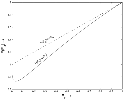
Figure 1: Two different functions $F(E_{R})$ of the relative entropy of entanglement $E_{R}$ are plotted. The continuous line shows the capacity C for SDC as a function of the relative entropy of entanglement $E_{R}$ if the initial shared state is a lambda state of the type A. The dashed line shows the function $1+E_{R}$. The figure illustrates that the capacity C for SDC is bounded from above by $1+E_{R}$

The plot of the classical capacity C for these states as a function of $E_{R}$ of the state has been shown in figure 1 and it is indeed found that

$${\bf\mbox{C}}\leq 1+E_{R}.$$ (72)

The equality holds true only at the two ends of the graph, namely at maximal entanglement $E_{R}=1$ (when $\sigma_{1}$ approaches a Bell state) and zero entanglement $E_{R}=0$ (when $\sigma_{1}$ approaches $|01\rangle\langle 01|$).

Next we look at states of the type [10]

$$\Lambda_{B}=\lambda|\Phi^{+}\rangle\langle\Phi^{+}|+(1-\lambda)|00\rangle\langle 00|$$ (73)

which we call lambda states of the type B. For these [10]

$$E_{R}(\Lambda_{B}) = s_{+}\log s_{+}+s_{-}\log s_{-}$$ (74)

$$- (1-\frac{\lambda}{2})\log(1-\frac{\lambda}{2})-\frac{\lambda}{2}\log\frac{\lambda}{2}\;\;,$$

where

$$s_{\pm}=\frac{1\pm\sqrt{1-2\lambda(1-\lambda)}}{2}$$ (75)

are the eigenvalues of $\Lambda_{B}$. The C for SDC in this case is given by

C $$= s_{+}\log s_{+}+s_{-}\log s_{-}$$ (76)

$$- (1-\frac{\lambda}{2})\log\frac{1}{2}(1-\frac{\lambda}{2})-\frac{\lambda}{2}\log\frac{\lambda}{4}.$$

As is clear from a simple comparison of Eqs.(74) and (76), for lambda states of the type B,

$${\bf\mbox{C}}=1+E_{R}.$$ (77)

Thus, a curious feature of lambda states of type B is that the capacity for SDC is actually always equal to $1+E_{R}$. We will discuss a bit more about this curious aspect later in the section.

Now we consider another special class of states called the Werner states [7, 21] parameterized by a number F called the fidelity [7] and given by

$$W_{F} = F|\Psi^{-}\rangle\langle\Psi^{-}|+\frac{1-F}{3}(|\Psi^{+}\rangle\langle\Psi^{+}|$$ (78)

$$+ |\Phi^{+}\rangle\langle\Phi^{+}|+|\Phi^{-}\rangle\langle\Phi^{-}|).$$

The relative entropy of entanglement of these states is given by [10]

$$E_{R}(W_{F})=F\log F+(1-F)\log(1-F)+1,$$ (79)

and the C for SDC is calculated to be

C $$= 2+F\log F+(1-F)\log\frac{(1-F)}{3}.$$ (80)

The plot C versus $E_{R}$ has been drawn in Fig.2 and it is found that even in this case,

$${\bf\mbox{C}}\leq 1+E_{R}.$$ (81)

Now consider the case of a general Bell diagonal state

$$B_{D} = \lambda_{1}|\Psi^{-}\rangle\langle\Psi^{-}|+\lambda_{2}|\Psi^{+}\rangle\langle\Psi^{+}|$$ (82)

$$+ \lambda_{3}|\Phi^{+}\rangle\langle\Phi^{+}|+\lambda_{4}|\Phi^{-}\rangle\langle\Phi^{-}|.$$

It has been proved in Ref.[8] that when all $\lambda_{i}\in[0,\frac{1}{2}]$ then

$$E_{R}(B_{D})=0,$$ (83)

while when any of the $\lambda_{i}$ (say $\lambda_{1}$) $\geq\frac{1}{2}$, then

$$E_{R}(B_{D})=\lambda_{1}\log\lambda_{1}+(1-\lambda_{1})\log(1-\lambda_{1})+1.$$ (84)

The C for SDC always turns out to be

$${\bf\mbox{C}}=2+\sum_{i}\lambda_{i}\log\lambda_{i}.$$ (85)

First consider the case when all $\lambda_{i}\in[0,\frac{1}{2}]$. From Eqs.(83) and (85) we find that

$$1+E_{R}(B_{D})-{\bf\mbox{C}} = -\sum_{i}\lambda_{i}\log\lambda_{i}-1$$ (86)

$$= -\sum_{i}\lambda_{i}(\log\lambda_{i}+1)$$

$$\geq 0,$$

where $\sum_{i}\lambda_{i}=1$ has been used to proceed from the first to the second step and $\log\lambda_{i}\leq-1$ (because $\lambda_{i}\in[0,\frac{1}{2}]$) has been used to proceed from the second to the third step.

Now consider the complementary case ($\lambda_{1}\geq\frac{1}{2}$). From Eqs.(84) and (85) we find that

$$1+E_{R}(B_{D})-{\bf\mbox{C}} = (1-\lambda_{1})\log(1-\lambda_{1})-\sum_{i\neq 1}\lambda_{i}\log\lambda_{i}$$ (87)

$$= (\sum_{i\neq 1}\lambda_{i})\log(\sum_{j\neq 1}\lambda_{j})-\sum_{i\neq 1}\lambda_{i}\log\lambda_{i}$$

$$= \sum_{i\neq 1}\lambda_{i}(\log(\sum_{j\neq 1}\lambda_{j})-\log\lambda_{i})$$

$$\geq 0,$$

where in order to proceed from the third to the fourth step we have used the simple fact that $\log(\lambda_{2}+\lambda_{3}+\lambda_{4})$ is greater than either of the terms $\log\lambda_{2}$,$\log\lambda_{3}$ or $\log\lambda_{4}$. Thus for all Bell diagonal states we have

$${\bf\mbox{C}}\leq 1+E_{R}.$$ (88)

Now we will point out a curious fact about the situation when any two of the eigenvalues of a Bell diagonal state (say $\lambda_{3}$ and $\lambda_{4}$) are zero. When $\lambda_{1}=\lambda_{2}=\frac{1}{2}$ (which means $E_{R}=0$), we have C$=1$ (using Eq.(85)). In all the other cases (for which we use Eqs.(84) and (85)) we have

$$1+E_{R}(B_{D})-{\bf\mbox{C}} = (1-\lambda_{1})\log(1-\lambda_{1})-\lambda_{2}\log\lambda_{2}$$ (89)

$$= 0,$$

where we have used the simple fact that $\lambda_{1}+\lambda_{2}=1$. Thus for all Bell diagonal states with only two nonzero eigenvalues we have

$${\bf\mbox{C}}=1+E_{R}.$$ (90)

On the basis of the results obtained in this section let us conjecture:

Conjecture : The C for SDC with completely general (possibly mixed) states is bounded from above by $1+E_{R}$.

A great deal of empirical evidence has been presented in this section in support of the conjecture. In the next section we proceed to give a heuristic justification in support of our conjecture. In fact, we will try to justify an even stronger upper bound on C.

9 SDC and purification

To justify the conjecture of the previous section, we will have to examine the following interesting question: How does the capacity C change if Alice and Bob first locally purify their ensemble and distill Bell states (following the optimal purification procedure) and follow this up by SDC? Various purification procedures have been described in Refs.[7, 11, 12, 13]. Here we assume that Alice and Bob follow the optimal purification process: One which helps them to distill the maximum fraction of Bell states from the initial ensemble. They will, after optimal purification, have a fraction $E_{D}$ (where $E_{D}$ is called the entanglement of distillation) shared pairs in Bell states and a fraction $(1-E_{D})$ pairs in a disentangled state. They now complete their ’purification’ process by converting the final subensemble of disentangled pairs to pure states by projective measurements. We refer to such a protocol as complete purification. After a complete purification, Alice can use the fraction $E_{D}$ of Bell pairs to send Bob information at the rate of 2 bits/pair and the fraction $(1-E_{D})$ of pure disentangled pairs to send information at the rate of 1 bit/pair. Thus if Alice and Bob initially shared $n$ pairs, the classical capacity after a complete and optimal purification procedure is

C $$= \frac{1}{n}\{2nE_{D}+n(1-E_{D})\}$$ (91)

$$= 1+E_{D}.$$

Note that the above result is only asymptotically true ($n\rightarrow\infty$). Naively, one might expect this C to be lower than the C before purification. This is because, as mentioned in Ref.[13], entanglement concentration is a more destructive process than quantum data compression. Some amount of shared entanglement is destroyed in the process of purification. So it might be expected that the final ensemble after a purification will be able to convey less classical information than the original ensemble. On the contrary, as we will justify, the capacity for SDC with the purified ensemble is greater than that with the unpurified ensemble when an optimal and complete purification protocol is used. The gain comes from the fact that now there are two separate sub-ensembles instead of a single ensemble. In this section, we will try to justify, albeit heuristically, the following statement (as a more fundamental conjecture than the one presented in the previous section):
Conjecture: The capacity for SDC is more when it is preceeded by a complete and optimal purification procedure.

We will first consider the special case of Bell diagonal mixed states, for which the proof of the increase in the SDC capacity on a complete and optimal purification (our conjecture) can be rigorously proved. For Bell diagonal states with entropy $S(\rho)\leq 1$, there is a purification protocol called hashing (with the distillable fraction being $E_{DH}=1-S(\rho)$) [7]. ¿From Eq.(85) we see that for these Bell diagonal states, the C for SDC is equal to $1+E_{DH}$. As hashing may not necessarily be the optimal protocol, we have $E_{DH}\leq E_{D}$. This immediately implies ${\bf\mbox{C}}\leq 1+E_{D}$. For the complementary case of Bell diagonal states with $S(\rho)>1$, we have (from Eq.(85) for SDC), ${\bf\mbox{C}}<1$. This is obviously less than $1+E_{D}$ for any finite value of the entanglement of distillation (i.e for all inseperable states [22]). Thus for all Bell diagonal states the C for SDC can be improved by a prior optimal and complete purification of the ensemble of shared states.

For the more general case of arbitrary mixed entangled states, the proof will, essentially, be heuristic. Our approach will be to split the change in the classical information capacity due to complete and optimal purification into two parts. The first part is positive (an increase in capacity) and due to the addition of classical side channels during the purification procedure. These side channels are used by Alice (A) to communicate the results of her measurements to Bob (B), or vice versa. As this communication during purification is already conveying information from A to B (or vice versa), the channel capacity of the classical side channels should be directly added to the classical capacity (of course, for this, we have to implicitly assume the additivity of classical capacities). The information conveyed from A to B (or vice versa) during purification is actually used by the two parties to precisely identify their entangled and disentangled subensembles. There is also a negative contribution (decrease in capacity) during the purification as a fraction $1-E_{D}$ of shared pairs loose all their entanglement. Of course a part of this entanglement is pumped into the entangled subensemble, but the remaining is lost. Our job will be to argue that the positive contribution in channel capacity due to addition of classical side channels outweighs the negative contribution due to loss of entanglement in an optimal and complete purification procedure.

Consider the process of purification as a process of information gain by A and B. Before the purification, both A and B have an equal amount of knowledge about their shared system (they both know the full density matrix). Finally, each of their shared states are pure (because of the completeness of the purification procedure) and both of them have equal knowledge (i.e each know which of the pairs form the disentangled subensemble and which of the pairs form the maximally entangled subensemble). Thus they have both gained an equal amount of information I/pair about their shared pairs during the process of purification. Now, acquiring a part of this information may not cause any destruction of shared entanglement (lets call it $\mbox{I}_{1}$/pair), while the remaining part (lets call it $\mbox{I}_{2}$/pair) does cause a lowering of shared entanglement. We now contend, that this part, $\mbox{I}_{2}$/pair has to be equal to the number of classical communication channels used in the optimal purification procedure. The logic follows from the fact that the optimal strategy would be for A and B to collaborate in such a way that both of them gain the entire information $\mbox{I}_{2}$/pair with the least destruction of entanglement. They must then each acquire only a fraction of the information complementary to the fraction acquired by the other. In this way, the total information acquired by A and B from the shared pairs through direct entanglement degrading measurements is $\mbox{I}_{2}$/pair. They can then use a minimum of $\mbox{I}_{2}$ classical side channels per pair to communicate their fraction of the acquired information to the other party. On the other hand, if each wanted to acquire a fraction of the total information by direct measurements which was not entirely complementary to the part acquired by the other, they would destroy more entanglement than is really necessary. Thus we would expect that the classical side channels contribute to boosting the capacity up by at least an amount $\mbox{I}_{2}$/pair in the optimal purification procedure.

Now consider how much the capacity decreases due to the degradation of shared entanglement during the purification procedure. The classical capacity of a fraction $1-E_{D}$ of the pairs drops from at most 2 bits/pair to 1 bit/pair (due to the completeness of the purification procedure, the final capacity cannot be lower than 1 bit/pair). Thus the drop in classical capacity of each of the finally disentangled pairs is not more than 1 bit. This implies that the net decrease in classical capacity of the entire ensemble due to loss of entanglement hasn’t been more than $1-E_{D}$ bits/pair.

When the information $\mbox{I}_{2}$ is greater than 1 bit/pair, the proof of our statement is straightforward. The increase in capacity due to classical side channels (i.e $\mbox{I}_{2}$/pair) is more than 1 bit/pair, while the decrease in capacity due to loss of entanglement is less than $1-E_{D}$ bits/pair. As $1-E_{D}$ is a fraction (i.e $1-E_{D}<1$), the increase in capacity on purification overrides the inevitable decrease in capacity due to degradation of shared entanglement. Clearly, thus the capacity to do SDC increases on prior purification when $\mbox{I}_{2}\geq 1$ bit.

Now, we have to show that no matter what the value of $\mbox{I}_{2}$ is, it is possible to find a purification protocol for which $\mbox{I}_{2}$ is greater than $1-E_{D}$ bits. In other words, if initially there are $n$ shared pairs (with $n$ being large), then the number of shared pairs which loose all their entanglement on gaining an information of $\mbox{I}_{2}$/pair can be made less than $n\mbox{I}_{2}$ by an appropriate choice of the purification protocol. From such a statement it directly follows that the increase in capacity on purification overrides the inevitable decrease in capacity due to degradation of shared entanglement. A simple way in which one may try to justify the above proposition is from the fact that one pair generally allows the extraction of upto two bits of information (one bit from each of A’s and B’s qubit). So, it should be possible, in general, to extract $n\mbox{I}_{2}$ amount of information from measurements on less than $n\mbox{I}_{2}$ shared pairs (whose entanglement is degraded). This intutive understanding leaves open the question as to whether the information $\mbox{I}_{2}$/pair relevant to purification can be acquired in this way. For that we resort to explicit exemplification. Consider the class of mixed states $\rho$ (having nonzero entropy $S(\rho)$) and a diagonal decomposition $\sum\lambda_{i}|\psi_{i}\rangle\langle\psi_{i}|$ in terms of the pure states $|\psi_{i}\rangle$. Also suppose that this diagonal decomposition does not coincide with the entanglement minimizing decomposition [20] of $\rho$. For such states, acquiring the information about the entropy ($S(\rho)$/pair) is essential during purification, as the final ensemble is pure. We now contend that acquiring this $S(\rho)$ /pair of information necessarily destroys some amount of shared entanglement. We will justify this by the method of contradiction. Suppose, it was really possible to acquire the information about the entropy $S(\rho)$ without destroying any entanglement. On acquiring an information of the amount equal to $S(\rho)$/pair, A and B will be able to divide their initial ensemble to four seperate pure subensembles, each being comprised of one of the states $|\psi_{i}\rangle$. The weight of each of these subensembles will be equal to the eigenvalues $\lambda_{i}$. The average entanglement shared by A and B after extracting the information $S(\rho)$/pair is thus $\sum\lambda_{i}E_{v}(|\psi_{i}\rangle)$. However, for the class of states $\rho$ that we are considering, $\sum\lambda_{i}E_{v}(|\psi_{i}\rangle)$ is necessarily greater than the initial shared entanglement (as quantified by the entanglement of formation $E_{F}$). Thus by purely local actions and classical communications, A and B have been able to increase the shared entanglement for these classes of mixed states. This contradicts the definition of entanglement as a quantity that cannot be increased by local actions and classical communications. Thus, mixed states with the diagonal decomposition not coincident with the entanglement minimizing decomposition cannot be locally purified without necessarily destroying some shared entanglement. Thus the information about the entropy of these states is of the type $\mbox{I}_{2}$ (i.e acquiring the information necessarily causes degradation of entanglement). A corollary which immediately follows (though not directly relevant to the main point of the paper), is: the optimal purification of mixed states with the diagonal decomposition not coincident with the entanglement minimizing decomposition necessarily has a nonzero $\mbox{I}_{2}$ and thus necessarily requires the use of classical side channels. Now consider such states when their entropy, and thereby $\mbox{I}_{2}$, exceeds $1$ bit. Thus the total information $n\mbox{I}_{2}$ needed to be acquired is greater than $n$ bits. However, purifiability (nonzero $E_{D}$) implies that the total entanglement loss can be entirely concentrated to the entanglement loss of $n(1-E_{D})$ pairs which is less than $n\mbox{I}_{2}$ pairs. Therefore, it is possible to gain the relevant $n\mbox{I}_{2}$ bits of information by destroying the entanglement of less than $n\mbox{I}_{2}$ pairs. Now we really need an unproven extension of the above statement: even when $\mbox{I}_{2}\leq 1$ bit and irrespective of the nature of the decomposition of $\rho$, it is possible to gain the relevant $n\mbox{I}_{2}$ amount of information by destroying the entanglement of less than $n\mbox{I}_{2}$ pairs. Though this may seem a large extrapolation, it seems highly plausible because one shared pair allows the extraction of upto two bits of information. Thus we would expect that, no matter what the value of $\mbox{I}_{2}$ is, the increase in capacity on purification overrides the inevitable decrease in capacity due to degradation of shared entanglement.

Thus the capacity to do SDC with the two pure subenembles (maximally entangled and fully disentangled) after a complete and optimal purification, is expected to be greater than the initial mixed (and uniformly entangled) ensemble. We thus conjecture, with the help of Eq.(91), the following bound on the capacity of doing SDC with any mixed entangled state

$${\bf\mbox{C}}\leq 1+E_{D}.$$ (92)

This is an even stronger upper bound on the classical capacity than the bound conjectured in the previous section as the relative entropy of entanglement $E_{R}$ is necessarily greater than $E_{D}$ [10]. From Eq.(92), it directly follows that ${\bf\mbox{C}}\leq 1+E_{R}$ (our previous conjecture). Note that in this section, this conjecture has been rigourously proved for all Bell diagonal states, heuristically proved for all states with entropy $S(\rho)\geq 1$ bit (i.e $\mbox{I}_{2}\geq 1$ bit) and shown to be highly plausible for other types of states.

10 Conclusion

In this paper we have obtained bounds on the capacity of doing dense coding in terms of the different measures of entanglement stemming from purification procedures. The rigorously proved part of the results of this paper is that for SDC one always has

$$E_{R}\leq{\bf\mbox{C}}\leq 1+E_{F}.$$ (93)

On the other hand if we allow for a conjecture (well supported by examples and heuristically justified in Section.9), we have the stronger result

$$E_{R}\leq{\bf\mbox{C}}\leq 1+E_{R}.$$ (94)

What is the significance of bounds on the C for SDC when it can be readily calculated? The importance can be realized when we invert the above equation and write

$${\bf\mbox{C}}-1\leq E_{R}\leq{\bf\mbox{C}}.$$ (95)

Thus by calculating (or measuring) the channel capacity for SDC, we can draw an inference about the range in which the entanglement of the shared states (as quantified by $E_{R}$) lies. Also one of the bounds, namely, ${\bf\mbox{C}}\leq 1+E_{F}$ continues to hold even when we are allowed to vary the a priori probability of the various signal states (GDC). Thus, our inequality allows one to impose a readily calculable (from the expression for $E_{F}$ in Ref.[20]) limit on the capacity for GDC, without having to optimize GDC over all possible a priori signal probabilities.

The physical interpretation of the upper bounds becomes clear from the considerations given in Section.9. During optimal and complete entanglement purification procedures one generally enhances the classical capacity much more due to added classical side channels than the inevitable decrease in capacity brought by the loss of entanglement. The information transferred through these classical side channels during purification helps to identify the entangled and disentangled subensembles. It is through this identification that they directly play the role of boosting the capacity. As after an optimal and complete entanglement purification procedure, the capacity is $1+E_{D}$, this post-purification capacity is an upper bound on the pre-purification capacity. As both the entanglement measures $E_{F}$ and $E_{R}$ are upper bounds on $E_{D}$, all our upper bounds follow immediately. It is interesting to note that the upper and the lower bounds are trivial in complementary regimes. When ${\bf\mbox{C}}\leq 1$, the upper bounds are trivial, but the lower bound ($E_{R}\leq{\bf\mbox{C}}$) is non trivial. On the other hand when ${\bf\mbox{C}}\geq 1$, the upper bounds are non trivial while the lower bound is trivial.

We believe that this paper imparts physical significance to the various measures of entanglement from the viewpoint of forming bounds on certain kinds of dense coding procedures. This direction of physical interpretation of the entanglement measures is very different from the standard interpretations which stem from entanglement dilution and distillation processes. In a sense, this paper links up the apparently disconnected notions of entanglement purification and dense coding. The considerations of the previous section implies the following lower bound on the distillable entanglement: $E_{D}\geq{\bf\mbox{C}}-1$. This is important because as yet there is no explicit formula for $E_{D}$ for a general mixed entangled state. Thus the readily calculable quantity ${\bf\mbox{C}}-1$ (in the case of SDC) may offer a convinient lower bound on the distillable entanglement of a given mixed state.

The interesting question to examine is what apart from entanglement is involved in determining the dense coding capacity. This may be some measure of distinguishability between the letter states (hinted by the fact that the average mutual distinguishability function forms an upper bound on the classical capacity C). An aim of further research should be to work towards a complete formula for the capacity of dense coding. Moreover, working with a similar motivation as this paper, one can also try to relate entanglement measures stemming from purification procedures to the other uses of shared entanglement such as teleportation [23] and secret key distribution [24].

11 Acknowledgements

We would like to thank Vladimir Buzek, Daniel Jonathan and Peter Knight for valuable discussions. This work is supported by the Inlaks Foundation, Elsag-Bailey, Hewlett-Packard, the European TMR networks ERB 4061PL951412 and ERBFMRXCT96066, the UK Engineering and Physical Sciences Research Council, the European Science Foundation and the Leverhume trust.

Figure 2: The continuous line shows how the capacity C for SDC varies with the relative entropy of entanglement $E_{R}$ of the initial shared Werner state. The dashed line shows that it is bounded from above by $1+E_{R}$

References

- [1] For a review see: Plenio, M. B., and Vedral, V., 1998, Cont. Phys., 39, 431.
- [2] Bennett, C. H., and Wiesner, S., 1992, Phys. Rev. Lett., 69, 2881.
- [3] Mattle, K., Weinfurter, H., Kwiat, P. G., and Zeilinger, A., 1996, Phys. Rev. Lett., 76, 4656.
- [4] Barenco A., and Ekert, A. K., 1995, J. Mod. Opt., 42, 1253.
- [5] Hausladen, P., Jozsa, R., Schumacher, B., Westmoreland, M., and Wootters, W. K., 1996, Phys. Rev. A, 54, 1869.
- [6] Bose, S., Vedral, V., and Knight, P. L., 1998, Phys. Rev. A, 57, 822.
- [7] Bennett, C. H., DiVincenzo, D. P., Smolin, J. A., and Wootters, W. K., 1996, Phys. Rev. A, 54, 3824.
- [8] Vedral, V., Plenio, M. B., Rippin, M. A., and Knight, P. L., 1997, Phys. Rev. Lett., 78, 574.
- [9] Vedral, V., Plenio, M. B., Jacobs, K., and Knight, P. L., 1997, Phys. Rev. A 56, 4452.
- [10] Vedral, V., Plenio, M. B., 1998, Phys. Rev., A 57, 1619.
- [11] Bennett, C. H., Brassard, G., Popescu, S., Schumacher, B., Smolin, J. A., and Wootters, W. K., 1996, Phys. Rev. Lett., 76, 722.
- [12] Deutsch, D., Ekert, A., Jozsa, R., Macchiavello, C., Popescu, S., and Sanpera, A., 1996, Phys. Rev. Lett., 77, 2818.
- [13] Bennett, C. H., Bernstein, H. J., Popescu, S., and Schumacher, B., 1996, Phys. Rev. A, 53, 2046.
- [14] Kholevo, A. S., 1973, Probl. Peredachi Inf, 9, 177 [Kholevo, A. S., 1973, Problems of Information Transmission, 9, 177 ]; The Holevo bound was first conjectured by: Gordon, J. P., 1964, Quantum Electronics and Coherent light, Proceedings of the International School of Physics ”Enrico Fermi,” Course XXXI, edited by P. A. Miles (Academic, New York), 156-181; Levitin, L. B., 1964, Information, Complexity and Control in Quantum Physics, edited by P. A. Miles, (Academic, New York), 111-115.
- [15] Ohya, M., 1989, Rep. Math. Phys., 27, 19; Hiai, F., and Petz, D., 1991, Comm. Math. Phys., 143, 99; Donald, M. J., 1986, Comm. Math. Phys., 105, 13; Donald, M. J., 1987, Math. Proc. Camb. Phil. Soc., 101, 363.
- [16] Holevo, A. S., 1998, IEEE Trans. Info. Th., 44, 269; Schumacher, B., Westmoreland, M. D., 1997, Phys. Rev. A, 56, 131.
- [17] Popescu, S., and Rohrlich, D., 1997, Phys. Rev. A, 56, R3319.
- [18] Horodecki, R., Horodecki, P., and Horodecki, M., 1995, Phys. Lett. A, 200, 340.
- [19] Rains, E. M., Entanglement purification via separable superoperators, 1997, LANL e-print quant-ph/9707002.
- [20] Wootters, W. K., 1998, Phys. Rev. Lett., 80, 2245.
- [21] Werner, R. F., 1989, Phys. Rev. A, 40, 4277.
- [22] Horodecki, M., Horodecki, P., and Horodecki, R., 1997, Phys. Rev. Lett., 78, 574.
- [23] Bennett, C. H., Brassard, G., Crepeau, C., Jozsa, R., Peres, A., and Wootters, W. K., 1993, Phys. Rev. Lett., 70, 1895.
- [24] Ekert, A. K., 1991, Phys. Rev. Lett., 67, 661.