Cumulant expansion for studying damped quantum solitons

Abstract

The quantum statistics of damped optical solitons is studied using cumulant-expansion techniques. The effect of absorption is described in terms of ordinary Markovian relaxation theory, by coupling the optical field to a continuum of reservoir modes. After introduction of local bosonic field operators and spatial discretization pseudo-Fokker-Planck equations for multidimensional $s$-parametrized phase-space functions are derived. These partial differential equations are equivalent to an infinite set of ordinary differential equations for the cumulants of the phase-space functions. Introducing an appropriate truncation condition, the resulting finite set of cumulant evolution equations can be solved numerically. Solutions are presented in a Gaussian approximation and the quantum noise is calculated, with special emphasis on squeezing and the recently measured spectral photon-number correlations [Spälter et al., Phys. Rev. Lett. 81, 786 (1998)].

I Introduction

The study of the nonclassical properties of optical pulses propagating in linear and nonlinear media has been a subject of increasing interest [1, 2, 3]. In particular effects such as quadrature-phase squeezing [1, 4, 5, 6, 7], photon-number squeezing [7, 8, 9, 10], intraspectral quantum correlations [11], and entanglement [12, 13] offer novel possibilities for optical communication and quantum nondemolition (QND) measurement [1, 2]. In this connection the development of reliable sources of nonclassical light has been of particular interest. Promising candidates for such sources have been nonlinear optical elements converting coherent light produced by lasers into nonclassical light.

Since nonclassical properties are always in competition with the noise associated with unavoidable losses, a quantum theoretical description is required that necessarily includes absorption. Numerous approaches to the problem of quantization of radiation in absorbing media have been made (see, e.g., [14] and references therein). In most quantization schemes the influence of absorption has been omitted. Concepts have been developed for both dispersionless [15, 16, 17, 18, 19, 20, 21, 22, 23, 24, 25, 26, 27, 28, 29, 30] and (weakly) dispersive media [4, 31, 32, 33, 34, 35, 36]. Formulations in which the medium is introduced macroscopically via a constant (i.e., frequency-independent) permittivity may run into problems when dispersion is present [15, 18, 24, 25]. The problem of quantization of radiation in dispersive and absorbing linear media has been considered in [37, 38, 39, 40, 41, 42, 43, 44, 45, 46]. Recently, the method of quantization via Green-function expansion [40], which is closely related to the (mesoscopic) diagonalization scheme considered in [39], has been extended to arbitrary linear media, i.e., arbitrarily space-dependent, Kramers-Kronig consistent permittivities [47, 48]. An extension of this approach to nonlinear, absorbing media has been given in [14]. An interesting attempt to treat the problem of quantization of radiation in dielectric media composed of two-level atoms has been considered in [36].

In this article the propagation of quantum solitons in absorbing nonlinear wave guides is studied. It is well known that nonlinear waveguides are promising tools for “turn-key” generation of nonclassical light [2], because of the great nonlinear interaction length and the high intensity of the radiation [3]. Moreover, the radiation can be well localized in space and time by forming solitonlike pulses. The stability of classical solitons in a lossless medium is based on the balance between anomalous group velocity dispersion and Kerr-induced self-phase modulation [49, 50]. The theoretical description of quantum solitons usually starts from a Hamiltonian, the classical form of which leads to the classical (optical) nonlinear Schrödinger equation [23, 27, 31, 32]. The quantum nonlinear Schrödinger equation (QNLSE) can be solved by means of the Bethe ansatz [32, 51, 52]. In practice, however, the QNLSE must be supplemented with further terms in order to describe effects such as absorption, third-order dispersion, and Raman scattering. Therefore methods based on the Hartree approximation [31, 53] and linearization around the classical solution [54, 55, 56, 57, 58] have been developed that also apply to the solution of modified QNLSE’s.

Alternatively, phase-space methods [59] can be applied [4, 60, 61, 62], starting from the master equation and introducing — after appropriate spatial discretization — high-dimensional phase-space functions that satisfy (pseudo-) Fokker-Planck equations (PFPE). The resulting nonlinear, high-dimensional, partial differential equations are hard to solve in general. In the case of proper FPE’s the solution can be tried to be obtained by stochastic simulation. In what follows cumulant expansion (see, e.g., [63, 64]) is used in order to derive an infinite set of evolution equations for the cumulant hierarchy associated with a chosen phase-space function. Introducing appropriate truncation, the resulting finite set of ordinary differential equations can then be solved numerically. The method is applied to damped optical quantum solitons in absorbing Kerr media, and numerical solutions in Gaussian approximation are presented. The quantum noise is calculated, with special emphasis on local and spectral squeezing [1, 4, 5, 6, 7, 8, 9, 10] and spectral photon-number correlation [11].

The article is organized as follows. In Sec. II the underlying master equation is given. The corresponding pseudo-Fokker-Planck equations for $s$-parametrized phase-space functions are derived in Sec. III. Section IV outlines the cumulant expansion and the derivation of the cumulant evolution equations. Numerical results of the solution in a Gaussian approximation are presented in Sec. V, and a summary and some concluding remarks are given in Sec VI.

II Master equation

In the simplest model absorption can be described in terms of Markovian relaxation theory, introducing in the QNLSE a linear damping term and an additive operator noise source associated with the losses [58, 61]. A more rigorous quantization scheme shows that the nonlinear interaction can also mix the field and the noise source to give a modified QNLSE with multiplicative noise terms [14]. Only for sufficiently weak absorption can the simple model of additive noise be applied. Here we will restrict our attention to this case.

Let us first consider pulse propagation in a lossless fiber. When the pulse is long compared to the optical period and spectrally well localized in an interval $\Delta k$ around the carrier wave number $k_{\rm c}$, then the dispersion relation $\omega(k)$ (of the linear wave equation) can be treated in a second-order approximation,

$$\omega(k_{{\rm c}}+k)\simeq\omega_{{\rm c}}+\omega^{(1)}k+{\textstyle\frac{1}{2}}\omega^{(2)}k^{2}.$$ (1)

Studying the nonlinear media it may be convenient to define the optical (mid)frequency $\bar{\omega}_{{\rm c}}$ slightly different from $\omega_{\rm c}$ given in Eq. (1)

$$\bar{\omega}_{{\rm c}}=\omega_{{\rm c}}-\delta\omega,\quad\delta\omega\ll\omega_{\rm c}.$$ (2)

Separating from the (positive- and negative-frequency parts of the) field the rapidly varying exponentials $\exp[\mp i(\bar{\omega}_{{\rm c}}t$ $\!-$ $\!k_{{\rm c}}z)]$, the pulse can be described in terms of slowly varying annihilation and creation operators $\hat{b}(z,t)$ and $\hat{b}^{\dagger}(z,t)$, respectively, that satisfy the equal-time commutation relations [14]

$$\left[\hat{b}(z,t),\hat{b}^{\dagger}(z^{\prime},t)\right]={\cal A}^{-1}\delta(z-z^{\prime}),$$ (3)

$$\left[\hat{b}(z,t),\hat{b}(z^{\prime},t)\right]=\left[\hat{b}^{\dagger}(z,t),\hat{b}^{\dagger}(z^{\prime},t)\right]=0$$ (4)

(${\cal A}$ is the effective cross section of the fiber). In what follows it will be convenient to use a reference frame that moves with the group velocity, i.e.,

$$z=v_{{\rm gr}}t+x,$$ (5)

where

$$v_{{\rm gr}}=\left.\frac{d\omega}{dk}\right|_{k=k_{c}}=\omega^{(1)},$$ (6)

and to introduce the operators

$$\hat{a}(x,t)=\hat{b}(v_{{\rm gr}}t+x,t),\quad\hat{a}^{\dagger}(x,t)=\hat{b}^{\dagger}(v_{{\rm gr}}t+x,t).$$ (7)

Obviously, the operators $\hat{a}(x,t)$ and $\hat{a}^{\dagger}(x,t)$ also satisfy commutation relations of the type given in Eqs. (3) and (4) [with $\delta(x$ $\!-$ $\!x^{\prime})$ in place of $\delta(z$ $\!-$ $\!z^{\prime})$].

Under the assumptions made, the undamped spatiotemporal pulse evolution is governed by the Hamiltonian [4, 23, 27, 31, 32]

$$\hat{H}=\hbar{\cal A}\int dx\,\left[\vphantom{a^{(2)}}\delta\omega\hat{a}^{\dagger}\hat{a}\right.$$ (9)

$$\quad\quad\quad+\left.{\textstyle\frac{1}{2}}\omega^{(2)}\left(\partial_{x}\hat{a}^{\dagger}\right)\left(\partial_{x}\hat{a}\right)+{\textstyle\frac{1}{2}}\chi\hat{a}^{\dagger}\hat{a}^{\dagger}\hat{a}\hat{a}\vphantom{a^{(2)}}\right],$$

where the constant ${\chi}$ is related to the third-order susceptibility $\chi^{(3)}$ as [4]

$${\chi}=\frac{3\chi^{(3)}\hbar(v_{{\rm gr}}k_{{\rm c}})^{2}}{4\epsilon_{{\rm r}}^{2}\epsilon_{0}}$$ (10)

($\epsilon_{{\rm r}}$ is the relative permittivity at frequency $\omega_{\rm c}$). Note that solitons can be formed either in focusing media with anomalous dispersion ($\chi$ $\!<$ $0$, $\omega^{(2)}$ $\!>$ $\!0$) or in defocusing media with normal dispersion ($\chi$ $\!>$ $\!0$, $\omega^{(2)}$ $\!<$ $\!0$).

Including in the theory damping as outlined above, the density operator (in the Schrödinger picture) satisfies the master equation

$$i\hbar~{}\partial_{t}\hat{\rho}=[\hat{H},\hat{\rho}]+i\gamma\hat{L}\hat{\rho},$$ (11)

where the Lindblad term [65]

$$\gamma\hat{L}\hat{\rho}=\gamma\hbar{\cal A}\int dx\,\left[\vphantom{a^{(2)}}N_{\rm th}\left(2\hat{a}^{\dagger}\hat{\rho}\hat{a}-\hat{\rho}\hat{a}\hat{a}^{\dagger}-\hat{a}\hat{a}^{\dagger}\hat{\rho}\right)\right.$$ (13)

$$\quad\quad\quad+\left.\left(N_{\rm th}+1\right)\left(2\hat{a}\hat{\rho}\hat{a}^{\dagger}-\hat{\rho}\hat{a}^{\dagger}\hat{a}-\hat{a}^{\dagger}\hat{a}\hat{\rho}\right)\vphantom{a^{(2)}}\right]$$

is responsible for damping, with $\gamma$ being the damping constant, and

$$N_{\rm th}=\left[\exp\left(\frac{\omega_{{\rm c}}\hbar}{k_{{\rm B}}T}\right)-1\right]^{-1}$$ (14)

($k_{{\rm B}}$ is the Boltzmann constant, $T$ the absolute temperature).

To obtain a discrete version of Eq. (11), we divide the $x$ interval into $m$ cells of size $\Delta x$ numbered with index $j$ and introduce discrete operators [61]

$$\hat{a}_{j}(t)=\sqrt{\frac{{\cal A}}{\Delta x}}\int_{x_{j}}^{x_{j}+\Delta x}dx\,\hat{a}(x,t),$$ (15)

with

$$x_{j}=\Delta x(j-[m/2]).$$ (16)

It follows from Eqs. (3) and (4) that the operators $\hat{a}_{j}$ and $\hat{a}_{j}^{\dagger}$ satisfy the equal-time commutation relations

$$\left[\hat{a}_{j}(t),\hat{a}_{j^{\prime}}^{\dagger}(t)\right]=\delta_{jj^{\prime}},$$ (17)

$$\left[\hat{a}_{j}(t),\hat{a}_{j^{\prime}}(t)\right]=\left[\hat{a}_{j}^{\dagger}(t),\hat{a}_{j^{\prime}}^{\dagger}(t)\right]=0.$$ (18)

When $\Delta x$ is sufficiently small, then Eq. (15) reduces to

$$\hat{a}_{j}(t)\simeq\hat{a}(x_{j},t)\sqrt{\Delta x{\cal A}},$$ (19)

and the relations for continuous quantities can be replaced with the relations for discrete quantities according to the rules

$$\int dx\,{\cal F}\!\left[\hat{a}(x),\hat{a}^{\dagger}(x)\right]$$ (22)

$$\hskip 17.22217pt\simeq\sum_{j}\Delta x\,{\cal F}\!\left[\hat{a}_{j}/\sqrt{\Delta x{\cal A}},\hat{a}_{j}^{\dagger}/\sqrt{\Delta x{\cal A}}\right],$$

$$\partial_{x}\hat{a}\simeq\frac{1}{\sqrt{\Delta x{\cal A}}}\frac{\hat{a}_{j+1}-\hat{a}_{j}}{\Delta x}\,,$$

where ${\cal F}[\hat{a}(x),\hat{a}^{\dagger}(x)]$ is an arbitrary function of $\hat{a}(x)$ and $\hat{a}^{\dagger}(x)$. Finally, it is often convenient to describe pulse propagation in terms of appropriately scaled quantities. In our numerical calculations we have used the scaled quantities given in Appendix A.

III Fokker-Planck equations

It is well known that the description of the quantum state in terms of the density matrix is fully equivalent to a description in terms of phase-space functions. In what follows we restrict our attention to $s$-parametrized phase-space functions [66, 67], which for $m$ operators $\hat{a}_{j}$ are functions of $m$ complex phase-space variables ${a}_{j}$. For notational convenience we will omit the time argument and write the phase-space arguments in a compact vector form

$$P(a_{1},a_{2},\ldots,a_{m},t;s)\equiv P({\bf a};s)=P({\bf u},{\bf v};s),$$ (23)

with the real vectors ${\bf u}$ and ${\bf v}$ being defined by

$${\bf a}={\bf u}+i{\bf v}.$$ (24)

Note that expectation values of $s$-ordered operator products are obtained by averaging the corresponding products of complex phase-space variables with the $s$-parametrized phase-space function, i.e.,

$$\langle\hat{a}_{1}^{\dagger}{{}^{n_{1}}}\dots\hat{a}_{m}^{\dagger}{{}^{\!\!\!n_{m}}}\hat{a}_{1}^{k_{1}}\dots\hat{a}_{m}^{k_{m}}\rangle_{s}$$ (27)

$$\hskip 8.61108pt=\int d^{m}{\bf u}\,d^{m}{\bf v}\,\big{[}\left(u_{1}-iv_{1}\right)^{n_{1}}\dots\left(u_{m}-iv_{m}\right)^{n_{m}}$$

$$\hskip 8.61108pt\times\left(u_{1}+iv_{1}\right)^{k_{1}}\dots\left(u_{m}+iv_{m}\right)^{k_{m}}\big{]}P({\bf u},{\bf v};s),$$

where the notation $\langle\hat{a}_{1}^{\dagger n_{1}}\dots\hat{a}_{m}^{k_{m}}\rangle_{s}$ is used to introduce $s$ ordering.

Applying standard rules (see, e.g., [68]), the evolution equation for $P({\bf u},{\bf v};s)$ can be derived from the master equation straightforwardly. After some algebra we obtain

  

$$\partial_{t}P({\bf u},{\bf v};s)=\sum_{j}\left\{\vphantom{\left[\frac{\partial}{\partial a_{j}^{*}}\right]}-\delta\omega\left[\frac{\partial}{\partial u_{j}}v_{j}-\frac{\partial}{\partial v_{j}}u_{j}\right]\right.-\frac{\omega^{(2)}}{2\Delta x^{2}}\left[\frac{\partial}{\partial u_{j}}(2v_{j}\!-\!v_{j+1}\!-\!v_{j-1})-\frac{\partial}{\partial v_{j}}(2u_{j}\!-\!u_{j+1}\!-\!u_{j-1})\right]$$ (30)

$$\hskip 8.61108pt+\,\bar{\chi}\left[\frac{\partial}{\partial u_{j}}v_{j}-\frac{\partial}{\partial v_{j}}u_{j}\right]\left(1\!-\!s\!-\!|a_{j}|^{2}\right)+\gamma\left[\frac{\partial}{\partial u_{j}}u_{j}+\frac{\partial}{\partial v_{j}}v_{j}\right]+{\bar{\chi}}\frac{1\!-\!s^{2}}{16}\left(\frac{\partial^{2}}{\partial u_{j}^{2}}+\frac{\partial^{2}}{\partial v_{j}^{2}}\right)\left(\frac{\partial}{\partial u_{j}}v_{j}-\frac{\partial}{\partial v_{j}}u_{j}\right)$$

$$\hskip 8.61108pt\left.+\,{\bar{\chi}}\frac{s}{2}\left[\left(\frac{\partial^{2}}{\partial u_{j}^{2}}-\frac{\partial^{2}}{\partial v_{j}^{2}}\right)u_{j}v_{j}-\frac{\partial}{\partial u_{j}}\frac{\partial}{\partial v_{j}}\left(u_{j}^{2}-v_{j}^{2}\right)\right]+\frac{\gamma}{2}\left(N_{\rm th}+\frac{1\!-\!s}{2}\right)\left(\frac{\partial^{2}}{\partial u_{j}^{2}}+\frac{\partial^{2}}{\partial v_{j}^{2}}\right)\vphantom{\left[\frac{\partial}{\partial a_{j}^{*}}\right]}\right\}P({\bf u},{\bf v};s)$$

  

[$\bar{\chi}$ $\!=$ $\!\chi/(\Delta x{\cal A})$]. An equation of this type is also called the pseudo-Fokker-Planck equation. Apart from the fact that in an ordinary FPE derivatives only up to second order appear [69], it is impossible, in general, to find a stochastic process that is equivalent to Eq. (30) and can be used for solving the equation. For $s$ $\!=$ $\!1$ ($P$ function) and $s$ $\!=$ $\!-1$ ($Q$ function) the two last terms in curly brackets in Eq. (30) correspond to noise with a nonpositive diffusion matrix which cannot be modeled by a stochastic process [4]. Nevertheless, such a PFPE can have nonsingular solutions (see, e.g., [70]). For $s$ $\!=$ $\!0$ (Wigner function) the fifth term in curly brackets in Eq. (30) contains so called third-order noise which also cannot be treated by stochastic simulation [71]. For all other values of $s$ the two terms appear together. It should be pointed out that for the so-called positive $P$ representation the master equation (11) corresponds to a proper FPE with positive definite diffusion matrix [4, 61, 72], so that stochastic simulation applies (see, e.g., [73]). However, the price to be paid is the doubling of variables.

IV Cumulant expansion

In order to solve Eq. (30), we apply cumulant expansion techniques. For this purpose we express the characteristic function of $P({\bf u},{\bf v};s)$ in terms of cumulants and derive the cumulant evolution equations. After appropriate truncation the set of ordinary differential equations can be solved numerically.

A Basic definitions

Let us consider a (quasi)probability distribution function $P({\bf q})$ $\!\equiv$ $P(q_{1},q_{2},\ldots,q_{f})$ of $f$ real variables $q_{k}$ and define its characteristic function $\chi(\underline{\bf q})$ $\!\equiv$ $\!\chi(\underline{q}_{1},\underline{q}_{2},\ldots,\underline{q}_{m})$ by the Fourier transform of $P({\bf q})$,

$$P({\bf q})=\frac{1}{(2\pi)^{f}}\int d^{f}\underline{\bf q}\,\chi(\underline{\bf q})e^{-i\underline{\bf q}\cdot{\bf q}},$$ (31)

$$\chi(\underline{\bf q})=\int d^{f}{\bf q}\,P({\bf q})e^{i\underline{\bf q}\cdot{\bf q}}.$$ (32)

From Eq. (32) it follows that the moments $\langle q_{1}^{n_{1}}\ldots q_{f}^{n_{f}}\rangle$ of the distribution function $P({\bf q})$ can be obtained from $\chi(\underline{\bf q})$ by differentiation,

$$\langle q_{1}^{n_{1}}\ldots q_{f}^{n_{f}}\rangle=\int d^{f}{\bf q}\,q_{1}^{n_{1}}\ldots q_{f}^{n_{f}}P({\bf q})$$ (34)

$$\hskip 25.83325pt=\left.\left(\frac{\partial}{i\partial\underline{q}_{1}}\right)^{n_{1}}\ldots\left(\frac{\partial}{i\partial\underline{q}_{f}}\right)^{n_{f}}\chi(\underline{\bf q})\right|_{\underline{\bf q}=0}$$

($n_{k}$ $\!\geq$ $\!0$). Hence, the Taylor-series expansion of the function $\chi(\underline{\bf q})$, which can be regarded as moment generating function, reads as

$$\chi(\underline{\bf q})=\sum_{\{n_{k}\}}\langle q_{1}^{n_{1}}\ldots q_{f}^{n_{f}}\rangle\,\frac{(i\underline{q}_{1})^{n_{1}}\ldots(i\underline{q}_{f})^{n_{f}}}{n_{1}!\ldots n_{f}!}\,.$$ (35)

Introducing the cumulant generating function $\Phi(\underline{\bf q})$,

$$\chi(\underline{\bf q})=e^{\Phi(\underline{\bf q})},$$ (36)

the cumulants $\langle\!\langle q_{1}^{n_{1}}\ldots q_{f}^{n_{f}}\rangle\!\rangle$ are defined by the Taylor-series expansion of $\Phi(\underline{\bf q})$ as follows:

$$\Phi(\underline{\bf q})=\sum_{\{n_{k}\}}\langle\!\langle q_{1}^{n_{1}}\ldots q_{f}^{n_{f}}\rangle\!\rangle\,\frac{(i\underline{q}_{1})^{n_{1}}\ldots(i\underline{q}_{f})^{n_{f}}}{n_{1}!\ldots n_{f}!}\,.$$ (37)

Combining Eqs. (35) – (37), the cumulants and moments can be related to each other as

$$\langle q_{1}^{n_{1}}\ldots q_{f}^{n_{f}}\rangle=\left(\frac{\partial}{\partial\underline{q}_{1}}\right)^{n_{1}}\ldots\left(\frac{\partial}{\partial\underline{q}_{f}}\right)^{n_{f}}$$ (39)

$$\hskip 8.61108pt\times\left.\exp\!\left[\sum_{\{k_{l}\}}\langle\!\langle q_{1}^{k_{1}}\ldots q_{f}^{k_{f}}\rangle\!\rangle\,\frac{\underline{q}_{1}^{k_{1}}\ldots\underline{q}_{f}^{k_{f}}}{k_{1}!\ldots k_{f}!}\right]\right|_{\underline{\bf q}=0},$$

$$\langle\!\langle q_{1}^{n_{1}}\ldots q_{f}^{n_{f}}\rangle\!\rangle=\left(\frac{\partial}{\partial\underline{q}_{1}}\right)^{n_{1}}\ldots\left(\frac{\partial}{\partial\underline{q}_{f}}\right)^{n_{f}}$$ (41)

$$\hskip 8.61108pt\times\left.\ln\!\left[\sum_{\{k_{l}\}}\langle q_{1}^{k_{1}}\ldots q_{f}^{k_{f}}\rangle\,\frac{\underline{q}_{1}^{k_{1}}\ldots\underline{q}_{f}^{k_{f}}}{k_{1}!\ldots k_{f}!}\right]\right|_{\underline{\bf q}=0}$$

($\langle\!\langle q_{1}^{0}\ldots q_{f}^{0}\rangle\!\rangle$ $\!=$ $\!0$). Note that the symmetry relations

$$\langle\ldots q_{i}^{n_{i}}\ldots q_{j}^{n_{j}}\ldots\rangle=\langle\ldots q_{j}^{n_{j}}\ldots q_{i}^{n_{i}}\ldots\rangle,$$ (42)

$$\langle\!\langle\ldots q_{i}^{n_{i}}\ldots q_{j}^{n_{j}}\ldots\rangle\!\rangle=\langle\!\langle\ldots q_{j}^{n_{j}}\ldots q_{i}^{n_{i}}\ldots\rangle\!\rangle$$ (43)

are valid. For a Gaussian distribution higher than second-order cumulants are equal to zero,

$$\langle\!\langle q_{1}^{n_{1}}\ldots q_{f}^{n_{f}}\rangle\!\rangle=0\quad\text{if}\quad n_{1}+\ldots+n_{f}>2,$$ (44)

so that higher than second-order moments can be expressed in terms of first- and second-order cumulants $\langle\!\langle q_{i}\rangle\!\rangle$ and $\langle\!\langle q_{i}q_{j}\rangle\!\rangle$, respectively (see, e.g., [71]).

Obviously, Eqs. (31) - (43) also apply to the $s$-parametrized phase-space functions $P({\bf u},{\bf v};s)$ introduced in Sec. III [$P({\bf q})$ $\!\to$ $\!P({\bf u},{\bf v};s)$, $\chi(\underline{\bf q})$ $\!\to$ $\!\chi(\underline{\bf u},\underline{\bf v};s)$, $\Phi(\underline{\bf q})$ $\!\to$ $\!\Phi(\underline{\bf u},\underline{\bf v};s)$]. Since the characteristic functions for different values of $s$ are related to each other as [67]

$$\chi(\underline{\bf u},\underline{\bf v};s)=\chi(\underline{\bf u},\underline{\bf v};s^{\prime})$$ (46)

$$\hskip 8.61108pt\times\,\exp\!\left[{\textstyle\frac{1}{8}}(s-s^{\prime})\left(\underline{u}_{1}^{2}+\underline{v}_{1}^{2}+\ldots+\underline{u}_{m}^{2}+\underline{v}_{m}^{2}\right)\right],$$

from Eqs. (36) and (37) it is seen that only the second-order cumulants of equal variables depend on $s$,

$$\langle\!\langle u_{j}u_{j^{\prime}}\rangle\!\rangle_{s} = \langle\!\langle u_{j}u_{j^{\prime}}\rangle\!\rangle_{s^{\prime}}-{\textstyle\frac{1}{4}}(s-s^{\prime})\delta_{jj^{\prime}}$$ (47)

and $\langle\!\langle v_{j}v_{j^{\prime}}\rangle\!\rangle_{s}$ accordingly. All other cumulants are independent of $s$ [63]. Note that the mean value of the complex amplitude $\langle\hat{a}_{j}\rangle$ and the intensity $I_{j}$ $\!\equiv$ $\!\langle\hat{a}^{\dagger}_{j}\hat{a}_{j}\rangle$ are given by

$$\langle\hat{a}_{j}\rangle=\langle\!\langle u_{j}\rangle\!\rangle_{s}+i\langle\!\langle v_{j}\rangle\!\rangle_{s},$$ (48)

$$I_{j}=\langle\!\langle u_{j}\rangle\!\rangle_{s}^{2}+\langle\!\langle v_{j}\rangle\!\rangle_{s}^{2}+\langle\!\langle u_{j}^{2}\rangle\!\rangle_{s}+\langle\!\langle v_{j}^{2}\rangle\!\rangle_{s}+{\textstyle\frac{1}{2}}(s-1)\,.$$ (49)

B Evolution equations

Let us assume that a (quasi)probability distribution function $P({\bf q})$ satisfies an evolution equation of the following type:

$$\partial_{t}P({\bf q})=\sum_{\{n_{l}\},\{k_{l}\}}\bigg{[}A_{n_{1}\ldots n_{f}}^{k_{1}\ldots k_{f}}$$ (51)

$$\hskip 17.22217pt\times\left(\frac{\partial}{\partial q_{1}}\right)^{n_{1}}q_{1}^{k_{1}}\ldots\left(\frac{\partial}{\partial q_{f}}\right)^{n_{f}}q_{f}^{k_{f}}\bigg{]}P({\bf q}),$$

where $A_{n_{1}\ldots n_{f}}^{k_{1}\ldots k_{f}}$ are constants. It follows from Eq. (51) that the characteristic function $\chi(\underline{\bf q})$, Eq. (32), satisfies the evolution equation

$$\partial_{t}\chi(\underline{\bf q})=\partial_{t}\int d^{f}{\bf q}\,e^{i\underline{\bf q}\cdot{\bf q}}P({\bf q})$$ (54)

$$\hskip 8.61108pt=\sum_{\{n_{l}\},\{k_{l}\}}\bigg{[}A_{n_{1}\ldots n_{f}}^{k_{1}\ldots k_{f}}(-i\underline{q}_{1})^{n_{1}}\ldots(-i\underline{q}_{f})^{n_{f}}$$

$$\hskip 17.22217pt\times\left(\frac{\partial}{i\partial\underline{q}_{1}}\right)^{k_{1}}\ldots\left(\frac{\partial}{i\partial\underline{q}_{f}}\right)^{k_{f}}\bigg{]}\chi(\underline{\bf q}),$$

and hence [see Eq. (36)]

$$\partial_{t}\Phi(\underline{\bf q})=e^{-\Phi(\underline{\bf q})}\!\!\!\!\sum_{\{n_{l}\},\{k_{l}\}}\!\!\bigg{[}A_{n_{1}\ldots n_{f}}^{k_{1}\ldots k_{f}}(-i\underline{q}_{1})^{n_{1}}\!\ldots(-i\underline{q}_{f})^{n_{f}}$$ (56)

$$\hskip 51.6665pt\times\left(\frac{\partial}{i\partial\underline{q}_{1}}\right)^{k_{1}}\ldots\left(\frac{\partial}{i\partial\underline{q}_{f}}\right)^{k_{f}}e^{\Phi(\underline{\bf q})}\bigg{]}.$$

Substituting for $\Phi(\underline{\bf q})$ in Eq. (56) the Taylor-series expansion (37) and comparing the coefficients of equal powers we arrive at

$$\partial_{t}\langle\!\langle q_{1}^{r_{1}}\ldots q_{f}^{r_{f}}\rangle\!\rangle=\sum_{\{n_{l}\},\{k_{l}\}}\bigg{[}A_{n_{1}\ldots n_{f}}^{k_{1}\ldots k_{f}}$$ (60)

$$\hskip 17.22217pt\times\,\frac{(-i)^{n_{1}+k_{1}+r_{1}}r_{1}!}{(r_{1}-n_{1})!}\ldots\frac{(-i)^{n_{f}+k_{f}+r_{f}}r_{f}!}{(r_{f}-n_{f})!}$$

$$\hskip 17.22217pt\times\left(\frac{\partial}{\partial\underline{q}_{1}}\right)^{r_{1}-n_{1}}\ldots\left(\frac{\partial}{\partial\underline{q}_{f}}\right)^{r_{f}-n_{f}}e^{-\Phi(\underline{\bf q})}$$

$$\hskip 17.22217pt\times\left(\frac{\partial}{\partial\underline{q}_{1}}\right)^{k_{1}}\ldots\left.\left(\frac{\partial}{\partial\underline{q}_{f}}\right)^{k_{f}}e^{\Phi(\underline{\bf q})}\bigg{]}\right|_{\underline{\bf q}=0}$$

($1/n!$ $\!\equiv$ $\!0$ if $n$ $\!<$ $\!0$). Performing in Eq. (60) the differentiations yields the cumulant evolution equations explicitly.

We now apply the scheme to the PFPE (30) in order to obtain the evolution equations of the cumulants associated with $P({\bf u},{\bf v};s)$. For the sake of clearness we somewhat change the notation, using $C_{u^{n}\cdots,v^{k}\cdots,\ldots}(x,x^{\prime},\ldots)$ to denote the cumulants (for chosen $s$), e.g.,

$$C_{uv,u^{2}}(x,x^{\prime})\equiv\langle\!\langle u_{j}v_{j}u_{j^{\prime}}^{2}\rangle\!\rangle_{s}\quad(j\neq j^{\prime}),$$ (61)

with $x$ $\!\equiv x_{j}$ [cf. Eq. (16); note that $x_{j\pm 1}$ $\!=$ $\!x\pm\Delta x$]. After some algebra the evolution equations for the first-order cumulants $C_{u}(x)$ and $C_{v}(x)$ are derived to be

$$\partial_{t}C_{u}(x)=-\gamma\,C_{u}(x)+\delta\omega\,C_{v}(x)$$ (66)

$$\hskip 8.61108pt+\,\frac{\omega^{(2)}}{2\Delta x^{2}}{\,\left[2\,C_{v}(x)-C_{v}(x\!-\!\Delta x)-C_{v}(x\!+\!\Delta x)\right]}$$

$$\hskip 8.61108pt+\,{\bar{\chi}}\,C_{v}(x)\left[{{C_{u}^{2}(x)}}\,+{{C_{v}^{2}(x)}}\right]$$

$$\hskip 8.61108pt+\,{\bar{\chi}}\,C_{v}(x)\left[(s-1)+C_{u^{2}}(x)+3C_{v^{2}}(x)\right]$$

$$\hskip 8.61108pt+\,2{\bar{\chi}}C_{u}(x)\,C_{uv}(x)+{\bar{\chi}}\left[C_{u^{2}v}(x)+C_{v^{3}}(x)\right],$$

$$\partial_{t}C_{v}(x)=-\gamma\,C_{v}(x)-\delta\omega\,C_{u}(x)$$ (71)

$$\hskip 8.61108pt+\,\frac{\omega^{(2)}}{2\Delta x^{2}}{\,\left[-2\,C_{u}(x)+C_{u}(x\!-\!\Delta x)+C_{u}({x}\!+\!\Delta x)\right]}$$

$$\hskip 8.61108pt-\,{\bar{\chi}}\,{{C_{u}(x)}}\left[{{C_{u}^{2}(x)}}\,+{{C_{v}^{2}(x)}}\right]$$

$$\hskip 8.61108pt-\,{\bar{\chi}}\,{{C_{u}(x)}}\left[(s-1)+3C_{u^{2}}(x)+C_{v^{2}}(x)\right]$$

$$\hskip 8.61108pt-\,2\,{\bar{\chi}}\,C_{v}(x)\,C_{uv}(x)-\,{\bar{\chi}}\left[C_{u^{3}}(x)+C_{uv^{2}}(x)\right].$$

Owing to the nonlinear interaction the first-order cumulants are coupled to second- and third-order cumulants, whose evolution equations are rather lengthy [for the evolution equations for the second-order cumulants, see Eqs. (B10) - (B29) in Appendix B]. Note that the right-hand sides of Eqs. (66), (71), and (B19) are $s$ independent [in accordance with Eq. (47) and the statement given there]. Note that in the limiting case $\Delta x$ $\!\rightarrow$ $\!0$ the cumulant evolution equations [cf. Eqs. (66), (71), and (B10)-(B29)] are transformed into partial differential equations for corresponding cumulant correlation functions.

C Gaussian approximation

With regard to a numerical treatment, the hierarchy of cumulant evolution equations, which represents an infinite set of coupled, nonlinear, ordinary, first-order differential equations, must be decomposed into finite, closed systems of equations. For this purpose approximation schemes are required to be applied. Note that only for the linear system (${\bar{\chi}}$ $\!=$ $\!0$) does the infinite set of equations decompose into finite, closed subsets, each of which contains cumulants of the same order.

For a sufficiently high peak photon number of the order of magnitude of $\bar{n}$ $\!\sim$ $\!10^{9}$ [Eq. (A9)] an expansion in $1/\bar{n}$ may be performed, in which the second-order cumulants are considered to be of magnitude $1/\bar{n}$ in comparison with the first-order cumulants and cumulants of higher than second order are neglected. Comparing terms of equal order we obtain a linear system of differential equations for the second-order cumulants, in which the first-order cumulants governed by truncated Eqs. (66) and (71) play the role of time-dependent coefficients (for such linearization schemes for lossless systems, see [4, 54, 55, 56, 57], and for absorbing case, e.g., [58]). The approximation scheme may be extended straightforwardly in order to also include higher-order cumulants in the calculation.

Another approach to the problem is to retain all cumulants up to some appropriately chosen order ${\cal N}$ and to set the remaining higher-order cumulants equal to zero. In what follows we restrict our attention to the second-order (Gaussian) approximation (${\cal N}$ $\!=$ $\!2$). Thus in Eqs. (66), (71), and (B10) – (B29) all terms that contain cumulants of third and fourth order are omitted, and the now closed system of nonlinear differential equations is solved numerically. This approximation obviously corresponds to the assumption that the quantum state of the pulse can be approximated by a Gaussian phase-space function $P({\bf u},{\bf v};s)$. Note that for Gaussian distributions higher than second order cumulants exactly vanish.

The Gaussian approximation may be expected to apply if the damping is not too small. To roughly estimate the range of validity of the Gaussian approximation, we note that the linearization approach used in [54] for an undamped fundamental quantum soliton fails at (scaled) times $\tilde{t}$ $\!\sim$ $\!\bar{n}^{1/4}$ [52] (for scaled quantities, see Appendix A). On the other hand, in absorbing media the soliton noise relaxes to thermal-equilibrium noise on a time scale $\sim$ $\!\tilde{\gamma}^{-1}$. As the non-Gaussian correlations are suppressed more rapidly than the Gaussian ones it is expected that for $\tilde{\gamma}^{-1}$ $\!\leq$ $\!\bar{n}^{1/4}$ the Gaussian approximation is valid for all times of pulse propagation. Hence, the lower limit for the scaled absorption coefficient is given by

$$\tilde{\gamma}\gtrsim\bar{n}^{-1/4},$$ (72)

which for $\bar{n}$ $\!\sim$ $\!10^{9}$ yields $\tilde{\gamma}$ $\!\gtrsim$ $\!5.6\times 10^{-3}$. For smaller values of $\tilde{\gamma}$ the Gaussian approximation is expected to be valid only in a limited time interval $\tilde{t}$ $\!\lesssim$ $\!\bar{n}^{1/4}$.

V Results

In the Gaussian approximation the steady-state solution of Eqs. (66), (71), and (B10) – (B29) can be found to be

$${C}_{u}(x)={C}_{v}(x)=0,$$ (73)

$${C}_{u,u}(x,x^{\prime})\!=\!{C}_{v,v}(x,x^{\prime})\!=\!\textstyle{\frac{1}{2}}\!\left[N_{\rm th}\!+\!\textstyle{\frac{1}{2}}(1\!-\!s)\right]\!\delta(x,x^{\prime}),$$ (74)

$${C}_{u,v}(x,x^{\prime})={C}_{v,u}(x,x^{\prime})=0$$ (75)

[$\delta(x,x^{\prime})$ $\!=$ $\!1$, if $|x$ $\!-$ $\!x^{\prime}|$ $\!\leq$ $\!\Delta x/2$, and $\delta(x,x^{\prime})$ $\!=$ $\!0$ otherwise]. It corresponds to thermal fluctuations, without any correlation between the fields at different space points. In the numerical solution of the time-dependent problem we have used the steady-state values (74) and (75) as initial values of the second-order cumulants. With regard to the initial values of the first-order cumulants, we have used the fundamental soliton solution of the classical nonlinear Schrödinger equation [49, 50],

$${C}_{u}(x) = \sqrt{n_{0}}\,\mathop{\rm sech}(x/x_{0}),$$ (76)

$${C}_{v}(x) = 0$$ (77)

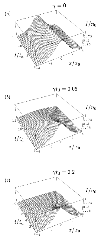
FIG. 1.: The spatiotemporal evolution of the intensity $I$ of a soliton is shown for various values of the damping constant $\gamma$.

[$n_{0}$ $\!=$ $\!\bar{n}\Delta x/x_{0}$, Eq. (A8)]. The initial conditions are realized by a multimode displaced thermal state, without entanglement between the modes corresponding to different space points (for displaced thermal states, see, e.g., [74]).

To be more specific, we have performed the calculations assuming a peak photon number of the initial pulse of $\bar{n}$ $\!=$ $\!10^{9}$ and a reservoir photon number of $N_{\rm th}$ $\!=$ $\!10^{-16}$ and setting the parameter $\delta\omega$ equal to zero. The value of $N_{\rm th}$ corresponds to a (vacuum) carrier wavelength of $\lambda_{\rm c}$ $\!=$ $\!2$ $\!\!\pi$ $\!\!c$ $\!\!/\omega_{\rm c}$ $\!=$ $1.5\,\mu{\rm m}$ of the pulse in vacuum and a temperature of $T$ $\!=$ $\!300$K [see Eq. (14)]. Thus the pulse is initially prepared in a displaced thermal state that is almost a coherent state. Assuming, e.g., losses of $\Gamma$ $\!=$ $0.3\,{\rm dB\,km}^{-1}$ [Eq. (A6)] and a fiber dispersive parameter of $D$ $\!=$ $20\,{\rm ps\,nm}^{-1}{\rm km}^{-1}$ [Eq. (A5)], the (scaled) damping constant is $\tilde{\gamma}$ $\!=$ $\!5.8\times 10^{-3}$ for a pulse duration of $t_{0}$ $\!=$ $2\,{\rm ps}$, and $\tilde{\gamma}$ $\!=$ $\!1.4\times 10^{-1}$ for $t_{0}$ $\!=$ $10\,{\rm ps}$, and the dispersion lengths are $x_{\rm d}$ $\!=$ $\!170\,{\rm m}$ and $x_{\rm d}$ $\!=$ $\!4.2\,{\rm km}$, respectively [see Eqs. (A2) – (A6)].

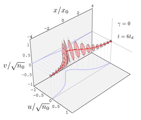
FIG. 2.: The local field fluctuations of an undamped soliton ($\gamma$ $\!=$ $\!0$) are shown for fixed propagation time $t$ and various positions $x$ in the pulse. The uncertainty ellipses in the phase space ($s$ $\!=$ $\!0.85$) are plotted in arbitrary units around the (solid line) complex amplitude $\langle\hat{a}(x)\rangle$ $\!=$ $\!\langle\hat{u}(x)\rangle$ $\!+$ $\!i\langle\hat{v}(x)\rangle$.

We have solved the equations numerically on a grid of $m$ $\!=$ $\!200$ points with $\Delta x$ $\!\!/x_{0}$ $\!=$ $\!0.1$ and absorbing boundary conditions, employing the Runge-Kutta method of order $8(5,3)$ with step-size control [75]. In order to test the program, we have performed the calculations for different values of $s$ and verified Eq. (47) to be within the numerical round-off error. Examples of the temporal evolution of the pulse intensity $I$ $\!=$ $\!I(x)$ $\!\equiv$ $\!I_{j}$, Eq. (49), are shown in Fig. 1 for various values of $\gamma$.

A Local fluctuations

In the Gaussian approximation, the local field noise (expressed in terms of $s$-ordered variances) can be visualized in phase space by means of uncertainty ellipses with the large $B^{1/2}$ and small $b^{1/2}$ axes and orientation angle $\varphi$,

$$B,b={\textstyle\frac{1}{2}}\left[C_{u^{2}}+C_{v^{2}}\pm\sqrt{\left(C_{u^{2}}-C_{v^{2}}\right)^{2}+4C_{uv}^{2}}\right],$$ (78)

$$2\varphi=\arg\left(C_{u^{2}}-C_{v^{2}}+2iC_{uv}\right)$$ (79)

(Appendix C), where the argument $x$ is skipped for simplicity. From inspection of Eqs. (78) and (79) together with Eq. (47) it can be seen that $b$ and $B$ depend on $s$,

$$b\to b_{s}=b_{0}-{\textstyle\frac{1}{4}}s$$ (80)

(and $B$ accordingly), whereas $\varphi$ is $s$ independent. The positions in phase space of the ellipses are determined by the $s$-independent first-order cumulants $C_{u}(x)$ and $C_{v}(x)$. Squeezed local fluctuations are observed if $b$ is reduced below the vacuum level $b_{\rm vac}$,

$$b<b_{\rm vac}\equiv{\textstyle\frac{1}{4}}(1-s)$$ (81)

(Appendix C). Obviously, the property of a state to be squeezed does not depend on $s$. For illustrational reasons it is convenient to choose $s$ as large as possible [otherwise the difference $b$ $\!-$ $\!(1$ $\!-$ $\!s)/4$ may not become visible].

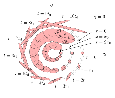
FIG. 3.: The temporal evolution of the local field fluctuations of an undamped soliton ($\gamma$ $\!=$ $\!0$) is shown for three typical positions in the pulse. The uncertainty ellipses in the phase space ($s$ $\!=$ $\!0.85$) are plotted in arbitrary units around the complex amplitude $\langle\hat{a}(x)\rangle$ $\!=$ $\!\langle\hat{u}(x)\rangle$ $\!+$ $\!i\langle\hat{v}(x)\rangle$. For comparison, the vacuum noise is indicated by circles.

The spatiotemporal evolution of the local field fluctuations (together with the complex amplitude) of an undamped soliton ($\gamma$ $\!=$ $\!0$, $\chi>0$, $\omega^{(2)}<0$) is illustrated in Figs. 2 and 3. Since the uncertainty ellipses are very small ($\sim\!n_{0}^{-1/2}$) compared with the (absolute) values of the complex amplitude ($\sim\!1$), the ellipses are plotted on an enlarged scale (of arbitrary units). Figure 2 represents the dependence on space of the local fluctuations for fixed time. The vacuum-noise level can be estimated from the uncertainties observed sufficiently far from the pulse center ($|x|$ $\!\gtrsim$ $4x_{0}$ in the figure), where the field is prepared in a state close to vacuum. The Kerr-induced self-phase modulation may be regarded as being the main reason for the enhanced phase noise of the field in the vicinity of the pulse center (for continuous wave radiation, see, e.g., [76]). The reason for the spatial redistribution of the local fluctuations may be seen in the dispersion that also leads to the observed enhanced amplitude noise at the wings of the pulse (for the influence of the dispersion on the squeezed pulses in linear media see, e.g., [77]). In Fig. 3 the temporal evolution of the local fluctuations is shown for various space points. It is seen that during the pulse propagation the complex amplitude rotates clockwise (counter-clockwise in the case $\chi<0$, $\omega^{(2)}>0$) in the phase space due to the nonlinear phase shift. The period of the rotation is close to the classical period $4\pi t_{\rm d}$ [50], because of the large value of $\bar{n}$. For small propagation times the field in the pulse center is squeezed, whereas at the wings the noise exceeds the vacuum level (indicated by the circles in the figure). In the further course of time an increase of the noise is observed.

FIG. 4.: The temporal evolution of the minimum-quadrature noise $b$ in the center of a soliton is shown for various values of the damping constant $\gamma$ ($s$ $\!=$ $\!0$).

The influence of absorption on the spatiotemporal evolution of the minimum quadrature noise $\!\sim$ $\!b$ is shown in Figs. 4 and 5. From Fig. 4 that presents the temporal evolution of $b$ in the pulse center it is seen that absorption reduces the maximally achievable amount of squeezing. Figure 5 reveals that for small propagation times ($t$ $\!\lesssim$ $\!t_{\rm d}$) squeezing is observed over the whole pulse, whereas in the further course of propagation ($t$ $\!\gtrsim$ $\!t_{\rm d}$) “noisy” wings appear owing to dispersion-assisted noise redistribution in the pulse. It is also seen that absorption reduces the effect of noise enhancement at the wings.

The local field noise can be described in terms of squeezed thermal states, and the squeezing condition (81) can be rewritten as

$$(2n+1)e^{-2r}<1$$ (82)

(Appendix C). Here, $n$ [Eq. (C8)] is the “thermal” photon number associated with the local field noise, and $r$ [Eq. (C9)] is the associated squeeze parameter. The parameter $r$ is a measure of the “deformation” of the uncertainty ellipses, whereas $n$ determines their “size”. Examples of the spatiotemporal evolution of $n$ and $r$ are shown in Figs. 6 and 7, respectively. It is seen that for small propagation times $r$ increases more rapidly than $n$ in the pulse center, and hence the field in the pulse center can be squeezed after the pulse has entered the fiber. The destructive influence of absorption is demonstrated in Figs. 6$(b)$ and 7$(b)$.

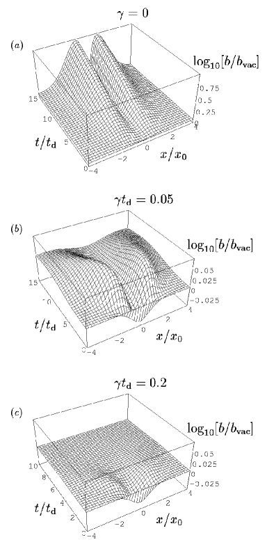
FIG. 5.: The influence of absorption on the spatiotemporal evolution of the minimum-quadrature noise $b$ of a soliton is illustrated for three values of the damping constant $\gamma$ ($s$ $\!=$ $\!0$).

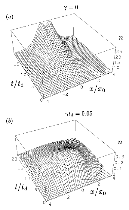
FIG. 6.: The spatiotemporal evolution of the “thermal” photon number $n$ of the squeezed thermal state associated with the local field noise of a soliton is shown for two values of the damping constant $\gamma$.

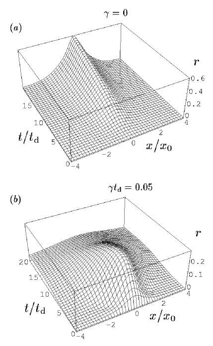
FIG. 7.: The spatiotemporal evolution of the squeeze parameter $r$ of the squeezed thermal state associated with the local field noise of a soliton is shown for two values of the damping constant $\gamma$.

B Squeezing spectrum

The squeezing spectrum of the (output) pulse can be measured using balanced homodyne detection [62]. Neglecting outcoupling effects, the temporal profile of the pulse after propagation through a fiber of length $L$ is described by the operator

$$\hat{a}(L-v_{\rm gr}t,t)=\hat{a}(-\tau v_{\rm gr},\tau+L/v_{\rm gr}),$$ (83)

where $\tau$ $\!=$ $\!t$ $\!-$ $\!L/v_{\rm gr}$ is the difference of the absolute time $t$ and the pulse arrival time $L/v_{\rm gr}$. The approximation in Eq. (1) requires the temporal pulse width $t_{0}$ to be small compared with the dispersion time $t_{\rm d}$, Eq. (A3),

$$t_{0}/t_{\rm d}\sim\Delta k|\omega^{(2)}|\,/\,|\omega^{(1)}|\ll 1.$$ (84)

Hence, the dependence on $\tau$ of the second argument in Eq. (83) can be ignored, and the time profile of the pulse can be described by

$$\hat{a}(-\tau v_{\rm gr},L/v_{\rm gr})=\hat{a}(x,L/v_{\rm gr})\equiv\hat{a}(x),$$ (85)

where for notational reasons the time coordinate $\tau$ is formally replaced by the spatial coordinate $x$

From Appendix D, the squeezing spectrum $S(\omega)$ can be expressed in terms of (discrete) $s$-ordered cumulants as

$$S(\omega)=2\mathop{\rm Re}\!\left[F_{\rm L}(-\omega,\omega)+e^{2i\varphi}G_{\rm L}(-\omega,\omega)\right]I_{0}^{-1},$$ (86)

where

$$F_{\rm L}(\omega,\omega^{\prime})=\frac{1}{2\pi}\sum_{jj^{\prime}}\Big{[}a_{{\rm L}\,j}^{*}a_{{\rm L}\,j^{\prime}}e^{i\omega x_{j}+i\omega^{\prime}x_{j^{\prime}}}$$ (87)

$$\hskip 17.22217pt\times\,\big{\{}\langle\!\langle u_{j}u_{j^{\prime}}\rangle\!\rangle_{s}+\langle\!\langle v_{j}v_{j^{\prime}}\rangle\!\rangle_{s}+{\textstyle\frac{1}{2}}(s-1)\delta_{jj^{\prime}}$$ (88)

$$\hskip 51.6665pt-i\left[\langle\!\langle u_{j}v_{j^{\prime}}\rangle\!\rangle_{s}-\langle\!\langle v_{j}u_{j^{\prime}}\rangle\!\rangle_{s}\right]\big{\}}\Big{]},$$ (89)

$$G_{\rm L}(\omega,\omega^{\prime})=\frac{1}{2\pi}\sum_{jj^{\prime}}\Big{[}a_{{\rm L}\,j}a_{{\rm L}\,j^{\prime}}e^{i\omega x_{j}+i\omega^{\prime}x_{j^{\prime}}}$$ (90)

$$\hskip 17.22217pt\times\,\big{\{}\langle\!\langle u_{j}u_{j^{\prime}}\rangle\!\rangle_{s}-\langle\!\langle v_{j}v_{j^{\prime}}\rangle\!\rangle_{s}$$ (91)

$$\hskip 51.6665pt-i\left[\langle\!\langle u_{j}v_{j^{\prime}}\rangle\!\rangle_{s}+\langle\!\langle v_{j}u_{j^{\prime}}\rangle\!\rangle_{s}\right]\big{\}}\Big{]}.$$ (92)

Here, $I_{0}$ is a normalization constant and $a_{{\rm L}\,j}$ is the complex local-oscillator (discrete) amplitude, with $\varphi$ being the relative phase between the local oscillator and the signal. Negative values of $S(\omega)$ signify squeezing at frequency $\omega$. Note that the squeezing spectrum involves internal pulse correlations expressed in terms of the two-argument cumulants in Eqs. (89) and (92). For the chosen frequency $\omega$ the minimum of $S(\omega)$,

$$S_{\min}(\omega)=2\left[\mathop{\rm Re}F_{\rm L}(-\omega,\omega)-|G_{\rm L}(-\omega,\omega)|\right]I_{0}^{-1},$$ (93)

is observed if the phase $\varphi$ is chosen such that

$$2\varphi=\pi-\arg\!\left[G_{\rm L}(-\omega,\omega)\right].$$ (94)

FIG. 8.: The influence of absorption on the temporal evolution of the midcomponent of the squeezing spectrum $S_{\min}(0)$, Eq. (86), is shown.

The temporal evolution of the minimum squeezing spectrum $S_{\min}(\omega)$ is shown in Figs. 8 and 9 ($\omega_{0}$ $\!=$ $2/x_{0}$). It is assumed that the local oscillator (LO) pulse has the shape of the initial fundamental-soliton pulse. Figure 8 demonstrates the influence of absorption on the temporal evolution of the squeezing spectrum for $\omega$ $\!=$ $\!0$, and examples of the full squeezing spectrum are shown in Fig. 9. At the initial stage of propagation wideband squeezing is observed which evolves to enhanced sideband noise in the further course of time [Figs. 9($a$) and 9($b$)]. From Fig. 9($a$) it is seen that in the lossless case the sidebands increase with time, whereas the midcomponent decreases (see also Fig. 8). Absorption introduces bounds, as can be seen from Fig. 9($b$). In particular, for sufficiently strong absorption the sidebands do not appear at all [Fig. 9($c$)].

It should be noted that in the numerical implementation of the $x$ integrals the value of $\Delta x$ imposes according to the sampling theorem [78] a condition on the upper bound of frequency: $|\omega|$ $\!\leq$ $\!\omega_{\rm max}$ $\!=$ $\!\pi(\Delta x)^{-1}$. Further, there is a minimally resolvable frequency difference $\Delta\omega_{\rm min}$ $\!=$ $\!2\pi(m\Delta x)^{-1}$. For $\Delta x/x_{0}$ $\!=$ $\!0.1$ and $m$ $\!=$ $\!200$ we find that $\omega_{\rm max}$ $\!=$ $\!5\pi$ $\!\omega_{0}$ and $\Delta\omega_{\rm min}$ $\!=$ $\!0.05\pi$ $\!\omega_{0}$.

C Spectral photon-number correlations

Recently experiments have been performed in order to measure the correlation of the number of photons $\hat{N}(\omega)$ at different frequencies [11]. A measure of the degree of correlation is the correlation coefficient

$$\eta(\omega,\omega^{\prime})\!=\!\frac{\langle:\!\Delta\hat{N}(\omega)\Delta\hat{N}(\omega^{\prime})\!:\rangle}{\big{[}\langle\Delta\hat{N}^{2}(\omega)\rangle\,\langle\Delta\hat{N}^{2}(\omega^{\prime})\rangle\big{]}^{1/2}}\,,$$ (95)

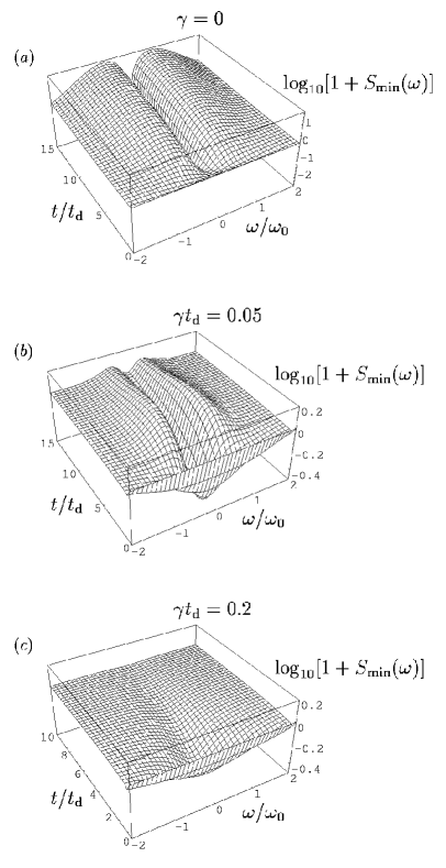
FIG. 9.: The temporal evolution of the squeezing spectrum $S_{\min}(\omega)$, Eq. (86), is shown for various values of the damping parameter $\gamma$.

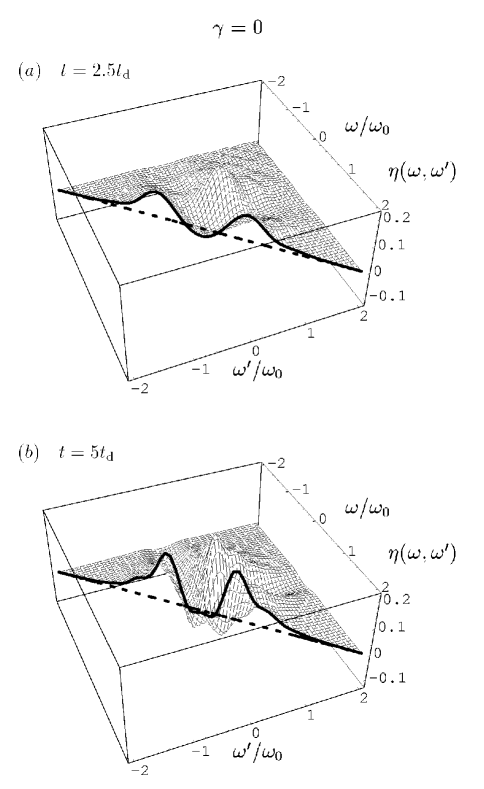
FIG. 10.: The photon-number correlation coefficient $\eta(\omega,\omega^{\prime})$, Eq. (95), of an undamped soliton ($\gamma$ $\!=$ $\!0$) is shown for two values of the propagation time $t$. Note that the symmetry relation $\eta(\omega,\omega^{\prime})$ $\!=$ $\eta(\omega^{\prime},\omega)$ is valid.

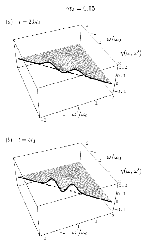
FIG. 11.: The photon-number correlation coefficient $\eta(\omega,\omega^{\prime})$, Eq. (95), of a damped soliton ($\gamma t_{\rm d}$ $\!=$ $\!0.05$) is shown for two values of the propagation time $t$. Note that the symmetry relation $\eta(\omega,\omega^{\prime})$ $\!=$ $\eta(\omega^{\prime},\omega)$ is valid.

where $\langle:\!\Delta\hat{N}(\omega)\Delta\hat{N}(\omega^{\prime})\!:\rangle$ is the normally ordered photon-number covariance, which is related to the ordinary covariance as

$$\langle\Delta\hat{N}(\omega)\Delta\hat{N}(\omega^{\prime})\rangle$$ (97)

$$\hskip 8.61108pt=\langle:\!\Delta\hat{N}(\omega)\Delta\hat{N}(\omega^{\prime})\!:\rangle+\langle\hat{N}(\omega)\rangle\delta(\omega,\omega^{\prime})$$

(Appendix E). The second term in Eq. (97), which represents a (quantum) shot-noise contribution, vanishes for $\omega$ $\!\neq$ $\omega^{\prime}$, and hence $\eta(\omega,\omega^{\prime})$ is the ordinary correlation coefficient. For $\omega$ $\!=$ $\omega^{\prime}$ the autocorrelation coefficient $\eta(\omega,\omega)$ is nothing but the (normalized) spectral photon-number variance in normal order. Negative (positive) values of $\eta(\omega,\omega)$ correspond to sub-Poisson (super-Poisson) photon-number statistics at chosen frequency $\omega$.

Expressing $\langle\hat{N}(\omega)\rangle$ and $\langle:\!\Delta\hat{N}(\omega)\Delta\hat{N}(\omega^{\prime})\!:\rangle$ in terms of (discrete) $s$-ordered cumulants yields

$$\langle\hat{N}(\omega)\rangle=\left[F(-\omega,\omega)+\left|E(\omega)\right|^{2}\right],$$ (98)

$$\langle:\!\Delta\hat{N}(\omega)\Delta\hat{N}(\omega^{\prime})\!:\rangle=\left|F(-\omega,\omega^{\prime})\right|^{2}+\left|G(\omega,\omega^{\prime})\right|^{2}$$ (100)

$$\hskip 4.30554pt+\,2\mbox{Re}\left[F(-\omega,\omega^{\prime})E(\omega)E^{*}\!(\omega^{\prime})+G(\omega,\omega^{\prime})E^{*}\!(\omega)E^{*}\!(\omega^{\prime})\right],$$

where

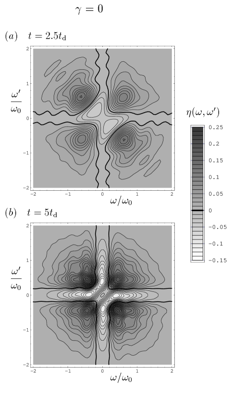
FIG. 12.: Contour plot of the photon-number correlation coefficient $\eta(\omega,\omega^{\prime})$, Eq. (95), of an undamped soliton for the same parameters as in Fig. 10.

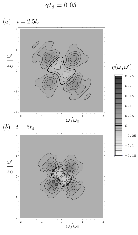
FIG. 13.: Contour plot of the photon-number correlation coefficient $\eta(\omega,\omega^{\prime})$, Eq. (95), of a damped soliton for the same parameters as in Fig. 11.

$$E(\omega)=\sqrt{\frac{\Delta x\Delta\omega}{2\pi}}\sum_{j}e^{i\omega x_{j}}\left[\langle\!\langle u_{j}\rangle\!\rangle_{s}+i\langle\!\langle v_{j}\rangle\!\rangle_{s}\right],$$ (102)

$$F(\omega,\omega^{\prime})=\frac{\Delta x\Delta\omega}{2\pi}\sum_{jj^{\prime}}e^{i\omega x_{j}+i\omega^{\prime}x_{j^{\prime}}}\big{\{}{\textstyle\frac{1}{2}}(s-1)\delta_{jj^{\prime}}$$ (104)

$$\hskip 4.30554pt+\,\langle\!\langle u_{j}u_{j^{\prime}}\rangle\!\rangle_{s}\!+\!\langle\!\langle v_{j}v_{j^{\prime}}\rangle\!\rangle_{s}\!+\!i\left[\langle\!\langle u_{j}v_{j^{\prime}}\rangle\!\rangle_{s}\!-\!\langle\!\langle v_{j}u_{j^{\prime}}\rangle\!\rangle_{s}\right]\big{\}},$$

$$G(\omega,\omega^{\prime})=\frac{\Delta x\Delta\omega}{2\pi}\sum_{jj^{\prime}}e^{i\omega x_{j}+i\omega^{\prime}x_{j^{\prime}}}\big{\{}\langle\!\langle u_{j}u_{j^{\prime}}\rangle\!\rangle_{s}$$ (106)

$$\hskip 34.44434pt-\,\langle\!\langle v_{j}v_{j^{\prime}}\rangle\!\rangle_{s}+i\left[\langle\!\langle u_{j}v_{j^{\prime}}\rangle\!\rangle_{s}+\langle\!\langle v_{j}u_{j^{\prime}}\rangle\!\rangle_{s}\right]\big{\}},$$

with $\Delta\omega$ being the resolving frequency (see Appendix E). We have performed the calculations choosing the minimally possible value of $\Delta\omega$ in the discretization scheme used (see the last paragraph in Sec. V B).

In Figs. 10 and 12 the correlation coefficient $\eta(\omega,\omega^{\prime})$ of an undamped soliton is plotted for two values of the propagation time $t$. The figures show typical features measured recently [11]. In particular, in the central part of the spectrum negative correlations are observed, whereas outside the center the frequency components can be strongly positively correlated. The negative values of the autocorrelation coefficient $\eta(\omega,\omega)$ (solid lines in Fig. 10) reveal, in agreement with [7], spectral sub-Poissonian statistics in the central part of the spectrum followed on both sides by regions of super-Poissonian statistics (dotted lines in Fig. 10 indicate the shot-noise level). With increasing propagation time the cross-correlation strength and the super-Poissonian autocorrelation strength are increased, whereas the sub-Poissonian autocorrelation effect becomes weaker [compare Figs. 10$(a)$ and 12$(a)$ for $t$ $\!=$ $\!2.5\,t_{\rm d}$ with Figs. 10$(b)$ and 12$(b)$ for $t$ $\!=$ $\!5\,t_{\rm d}$ respectively].

In Figs. 11 and 13 the correlation coefficient $\eta(\omega,\omega^{\prime})$ of a damped soliton is shown for the same values of the propagation time as in Figs. 10 and 12. Whereas in the early stage of propagation similar results are observed [compare Figs. 10$(a)$ and 12$(a)$ with Figs. 11$(a)$ and 13$(a)$, respectively], in the further course of time both the negative and positive cross correlations are smeared owing to damping [compare Figs. 10$(b)$ and 12$(b)$ with Figs. 11$(b)$ and 13$(b)$, respectively]. In contrast to the cross correlations, the effect of sub-Poissonian autocorrelations in the center of the spectrum can be stronger for the damped soliton than for the undamped one. This surprising effect may be a result of damping out destructive fluctuation interferences that occur for vanishing damping.

As mentioned above, from the theory sub-Poissonian statistics is expected to occur in the central part of the spectrum. Further the calculation yields a correlation coefficient that fulfills the symmetry relation $\eta(\omega,\omega^{\prime})$ $\!=$ $\!\eta(-\omega,-\omega^{\prime})$. The two effects have not been observed in the experiment in [11]. A reason for the discrepancies may be seen in phonon-scattering-induced noise which is not considered here. It should be mentioned that for small damping an observable sub-Poissonian effect is expected to occur only at a rather early stage of pulse propagation [Figs. 10$(a)$ and 12$(a)$].

VI Summary and concluding remarks

We have studied the influence of absorption on the quantum statistics of optical solitons in Kerr media, introducing multivariable $s$-parametrized phase-space distributions for describing the multimode quantum state of a solitonlike pulse. The evolution equations for the phase-space distributions can be tried to be solved using cumulant-expansion techniques. When the damping is not too small, then the quantum state can be treated in Gaussian approximation; i.e., only cumulants up to second order are to be taken into account. Otherwise, the evolution time must not be too large. Starting with an undamped fundamental soliton prepared in a nearly coherent state, we have solved the set of differential equations in Gaussian approximation numerically. From the solution, we have analyzed the local field fluctuations in terms of minimum-quadrature noise and squeezed thermal states, and we have calculated the squeezing spectrum and the spectral photon-number correlation coefficient.

The cumulant evolution equations in the rigorous Gaussian approximation used in this article contain nonlinear terms that are disregarded in the linearization approximation. The obtained results show that for sufficiently big coherent amplitude the Gaussian approximation closely corresponds to the linearization approximation. Deviations of the exact behavior of the quantum noise from the behavior obtained in the linearization approximation may therefore be regarded as being of non-Gaussian type. In this way, the cumulant method offers a possibility of improving the theory, including in it higher-order cumulants — at least third-order cumulants — for describing the non-Gaussian effects in a consistent way.

The method can of course be used in order to study further aspects of damped quantum soliton motion. For example, the class of initial conditions can be extended. In practice, the pulses which are fed into a fiber are not of the fundamental-soliton type in general. Further, sequences of pulses can give rise to interactions between them. When the losses are very small, then non-Gaussian effects may be observable, which requires inclusion in the theory of higher than second-order cumulants. The model of the Kerr medium can also be improved by including effects like Raman and Brillouin scattering [61], third-order dispersion [53], and frequency-dependent absorption. In order to further specify the nonclassical features of solitonlike pulses under realistic conditions and compare the quantum motion with the classical one, additional properties must be studied. With regard to the multimode structure of solitons, the study of nonclassical internal pulse correlations plays an important role. Finally, application to other systems is also possible, e.g., solitons in $\chi^{(2)}$ media [62], self-induced transparency solitons [79], or video pulses [80].

 

A Scaled variables

The scaled coordinates $\tilde{x}$ and $\tilde{t}$ are defined by

$$\tilde{x} = \frac{x}{x_{0}}\,,$$ (A1)

$$\tilde{t} = \frac{t}{t_{\rm d}}\,,$$ (A2)

where $x_{0}$ is the spatial pulse width, and $t_{\rm d}$ is the dispersion time, which is related to the dispersion length $x_{\rm d}$ as

$$t_{\rm d}=\frac{x_{d}}{v_{\rm gr}}\,,$$ (A3)

and $x_{\rm d}$ can be given by [50]

$$x_{\rm d}=\frac{t_{0}^{2}}{|k^{(2)}|}=\frac{x_{0}^{2}v_{\rm gr}}{|\omega^{(2)}|}\,,$$ (A4)

where $t_{0}$ $\!=$ $\!x_{0}/v_{\rm gr}$ is the temporal pulse width and

$$k^{(2)}=-\frac{\omega^{(2)}}{v_{\rm gr}^{3}}=-2\pi\,\frac{cD}{\omega_{\rm c}^{2}}$$ (A5)

[for $\omega^{(2)}$ and $v_{\rm gr}$, see Eqs. (1) and (6)]. In Eq. (A5), the (fiber) dispersive parameter $D$ is introduced [50]. Further the scaled damping parameter $\tilde{\gamma}$ is defined by

$$\tilde{\gamma}=\gamma\,t_{\rm d}=0.05\cdot\ln\!10\cdot\Gamma\,[{\rm dB}\,{\rm km}^{-1}]\cdot x_{\rm d}\,[{\rm km}].$$ (A6)

Finally the scaled amplitude operators

$$\tilde{\hat{a}}_{j}=\frac{\hat{a}_{j}}{\sqrt{n_{0}}}$$ (A7)

are introduced, where

$$n_{0}=\bar{n}\,\frac{\Delta x}{x_{0}}\,.$$ (A8)

Here

$$\bar{n}=\left|\frac{\omega^{(2)}{\cal A}}{\chi x_{0}}\right|$$ (A9)

is a measure of the initial photon number of the pulse [4, 61] and is typically of the order of magnitude of $10^{8}$ – $10^{9}$ for solitons in optical fibers [1].

B Evolution equations for the second-order cumulants

Using the notation introduced in Eq. (61), the evolution equations for the second-order cumulants read as

  

$$\partial_{t}C_{u,u}(x,x^{\prime})=\left\{\gamma\,\left(N_{\rm th}+{\frac{1-s}{2}}\right)+s{\bar{\chi}}\left[C_{u}(x)\,C_{v}(x)+C_{uv}(x)\right]\right\}\delta(x,x^{\prime})$$ (B1)

$$\quad-2\,\gamma\,C_{u,u}(x,x^{\prime})+\delta\omega\,C_{u,v}(x,x^{\prime})+\delta\omega\,C_{v,u}(x,x^{\prime})$$ (B2)

$$\quad-\frac{\omega^{(2)}}{2\Delta x^{2}}\left[C_{u,v}(x,x^{\prime}-{\Delta x})-2\,C_{u,v}(x,x^{\prime})+C_{u,v}(x,x^{\prime}+{\Delta x})\right]$$ (B3)

$$\quad-\frac{\omega^{(2)}}{2\Delta x^{2}}{\left[C_{v,u}(x-{\Delta x},x^{\prime})-2\,C_{v,u}(x,x^{\prime})+C_{v,u}({x}+{\Delta}x,x^{\prime})\right]}$$ (B4)

$$\quad+{\bar{\chi}}\Big{\{}C_{u,v}(x,x^{\prime})\left[C_{u}^{2}{{(x^{\prime})}}+3\,C_{v}^{2}{{(x^{\prime})}}\right]+C_{v,u}(x,x^{\prime})\left[C_{u}^{2}{(x)}+3\,C_{v}^{2}{(x)}\right]$$ (B5)

$$\quad\quad\quad+C_{u,v}(x,x^{\prime})\left[(s-1)+C_{u^{2}}(x^{\prime})\,+3\,C_{v^{2}}(x^{\prime})\right]+C_{v,u}(x,x^{\prime})\left[(s-1)+C_{u^{2}}(x)+3\,C_{v^{2}}(x)\right]$$ (B6)

$$\quad\quad\quad+2\,C_{u,u}(x,x^{\prime})\left[C_{u}(x)\,C_{v}(x)\,+C_{u}(x^{\prime})\,C_{v}(x^{\prime})+C_{uv}(x)+C_{uv}(x^{\prime})\right]$$ (B7)

$$\quad\quad\quad+C_{v}(x)\,C_{u^{2},u}(x,x^{\prime})+C_{v}(x^{\prime})\,C_{u,u^{2}}(x,x^{\prime})+2\,C_{u}(x^{\prime})\,C_{u,uv}(x,x^{\prime})$$ (B8)

$$\quad\quad\quad+3\,C_{v}(x^{\prime})\,C_{u,v^{2}}(x,x^{\prime})+2\,C_{u}(x)\,C_{uv,u}(x,x^{\prime})+3\,C_{v}(x)\,C_{v^{2},u}(x,x^{\prime})$$ (B9)

$$\quad\quad\quad+C_{u,u^{2}v}(x,x^{\prime})+C_{u,v^{3}}(x,x^{\prime})+C_{u^{2}v,u}(x,x^{\prime})+C_{v^{3},u}(x,x^{\prime})\Big{\}},$$ (B10)

$$\partial_{t}C_{u,v}(x,x^{\prime})={\bar{\chi}}\left[C_{u^{2}}^{2}{(x)}-C_{v^{2}}^{2}{(x)}\right]\delta(x,x^{\prime})-2\,\gamma\,C_{u,v}(x,x^{\prime})+\delta\omega\,C_{v,v}(x,x^{\prime})-\delta\omega\,C_{u,u}(x,x^{\prime})$$ (B11)

$$\quad+{\frac{s\,}{2}\bar{\chi}}\left[C_{v}^{2}{{(x)}+}C_{v^{2}}(x){-}C_{u}^{2}{(x)}-C_{u^{2}}(x)\right]\delta(x,x^{\prime})$$ (B12)

$$\quad+{\frac{\omega^{(2)}}{2\Delta x^{2}}\,\left[C_{u,u}(x,x^{\prime}-{\Delta x})-2\,C_{u,u}(x,x^{\prime})+C_{u,u}(x,x^{\prime}+{\Delta x})\right]}$$ (B13)

$$\quad-\frac{\omega^{(2)}}{2\Delta x^{2}}{\,\left[C_{v,v}(x-{\Delta x},x^{\prime})-2\,C_{v,v}(x,x^{\prime})+C_{v,v}({x}+{\Delta}x,x^{\prime})\right]}$$ (B14)

$$\quad+{\bar{\chi}}\left\{-C_{u,u}(x,x^{\prime})\left[3\,C_{u}^{2}{{(x^{\prime})}}+C_{v}^{2}{{(x^{\prime})}}\right]+C_{v,v}(x,x^{\prime})\left[C_{u}^{2}{(x)}+3\,C_{v}^{2}{(x)}\right]\right.$$ (B15)

$$\quad\quad-C_{u,u}(x,x^{\prime})\left[\left(s-1\right)+3\,C_{u^{2}}(x^{\prime})\,+C_{v^{2}}(x^{\prime})\right]+C_{v,v}(x,x^{\prime})\left[\left(s-1\right)+C_{u^{2}}(x)\,+3\,C_{v^{2}}(x)\right]$$ (B16)

$$\quad\quad+2\,C_{u,v}(x,x^{\prime})\,\left[C_{u}(x)\,C_{v}(x)+C_{uv}(x)-C_{u}(x^{\prime})\,C_{v}(x^{\prime})-C_{uv}(x^{\prime})\right]$$ (B17)

$$\quad\quad-C_{u}(x^{\prime})\,C_{u,v^{2}}(x,x^{\prime})+2\,C_{u}(x)\,C_{uv,v}(x,x^{\prime})+3\,C_{v}(x)\,C_{v^{2},v}(x,x^{\prime})$$ (B18)

$$\quad\quad\left.-C_{u,u^{3}}(x,x^{\prime})-C_{u,uv^{2}}(x,x^{\prime})+C_{u^{2}v,v}(x,x^{\prime})+C_{v^{3},v}(x,x^{\prime})\right\},$$ (B19)

$$\partial_{t}C_{v,v}(x,x^{\prime})=\left\{\gamma\,\left(N_{\rm th}+{\frac{1-s}{2}}\right)-s{\bar{\chi}}\left[C_{u}(x)\,C_{v}(x)+C_{uv}(x)\right]\right\}\delta(x,x^{\prime})$$ (B20)

$$\quad-2\,\gamma\,C_{v,v}(x,x^{\prime})-\delta\omega\,C_{u,v}(x,x^{\prime})-\delta\omega\,C_{v,u}(x,x^{\prime})$$ (B21)

$$\quad+\frac{\omega^{(2)}}{2\Delta x^{2}}{\,\left[C_{u,v}(x-\Delta x,x^{\prime})-2\,C_{u,v}(x,x^{\prime})+C_{u,v}({x}+{\Delta}x,x^{\prime})\right]}$$ (B22)

$$\quad+{\frac{\omega^{(2)}}{2\Delta x^{2}}\,\left[C_{v,u}(x,x^{\prime}-\Delta x)-2\,C_{v,u}(x,x^{\prime})+C_{v,u}(x,x^{\prime}+{\Delta x})\right]}$$ (B23)

$$\quad-{\bar{\chi}}\left\{C_{u,v}(x,x^{\prime})\left[3\,C_{u}^{2}{(x)}+C_{v}^{2}{(x)}\right]+C_{v,u}(x,x^{\prime})\left[3\,C_{u}^{2}{{(x^{\prime})}}+C_{v}^{2}{{(x^{\prime})}}\right]\right.$$ (B24)

$$\quad\quad+C_{u,v}(x,x^{\prime})\left[\left(s-1\right)+3\,C_{u^{2}}(x)+\,C_{v^{2}}(x)\,\right]+C_{v,u}(x,x^{\prime})\left[\left(s-1\right)+3\,C_{u^{2}}(x^{\prime})+\,C_{v^{2}}(x^{\prime})\right]$$ (B25)

$$\quad\quad+2\,C_{v,v}(x,x^{\prime})\left[C_{u}(x)\,C_{v}(x)\,+\,C_{u}(x^{\prime})\,C_{v}(x^{\prime})+C_{uv}(x)+C_{uv}(x^{\prime})\right]$$ (B26)

$$\quad\quad+2\,C_{v}(x)\,C_{uv,v}(x,x^{\prime})+2\,C_{v}(x^{\prime})\,C_{v,uv}(x,x^{\prime})+C_{u}(x)\,C_{v^{2},v}(x,x^{\prime})$$ (B27)

$$\quad\quad+3\,C_{u}(x)\,C_{u^{2},v}(x,x^{\prime})+3\,C_{u}(x^{\prime})\,C_{v,u^{2}}(x,x^{\prime})+C_{u}(x^{\prime})\,C_{v,v^{2}}(x,x^{\prime})$$ (B28)

$$\quad\quad\left.+C_{u^{3},v}(x,x^{\prime})+C_{v,u^{3}}(x,x^{\prime})+C_{v^{2}u,v}(x,x^{\prime})+C_{v,v^{2}u}(x,x^{\prime})\right\}.$$ (B29)

  

C Squeezed thermal noise

For chosen $x$ the (single-mode) $s$-parametrized characteristic function $\chi(\underline{u},\underline{v};s)$ of the local noise in Gaussian approximation,

$$\chi(\underline{u},\underline{v};s)=\exp\!\left[-{\textstyle\frac{1}{2}}\left(C_{u^{2}}\underline{u}^{2}+2C_{uv}\underline{u}\,\underline{v}+C_{v^{2}}\underline{v}^{2}\right)\right],$$ (C1)

can be rewritten as

$$\chi(\underline{u},\underline{v};s)=\exp\!\left[-{\textstyle\frac{1}{2}}\left(B\underline{u}^{\prime}{{}^{2}}+b\underline{v}^{\prime}{{}^{2}}\right)\right],$$ (C2)

$$\underline{u}^{\prime}+i\underline{v}^{\prime}=(\underline{u}+i\underline{v})e^{i\varphi}\,,$$ (C3)

where $B$, $b$, and $\varphi$, respectively, are given in Eqs. (78) and (79). The characteristic function $\chi(\underline{u},\underline{v};s)$ corresponds to a squeezed thermal state

$$\hat{\rho}=\hat{S}(\xi)\,\hat{\rho}_{\rm th}(n)\,\hat{S}^{\dagger}(\xi),$$ (C4)

which is obtained by applying the squeeze operator

$$\hat{S}(\xi) = \exp\!\left[{\textstyle\frac{1}{2}}\left(\xi^{*}\hat{a}^{2}-\xi\hat{a}^{\dagger}{{}^{\,2}}\right)\right]$$ (C5)

on a thermal state $\hat{\rho}_{\rm th}(n)$ of mean photon number $n$ (for squeezed thermal states, see, e.g.,[74]). The second-order cumulant parameters in Eq. (C1) can be shown to be related to the parameters $\xi$ $\!=$ $\!re^{i\theta}$ and $n$ in Eq. (C4) as

$$C_{u^{2}}+C_{v^{2}}=\left(n+{\textstyle\frac{1}{2}}\right)\cosh(2r)-{\textstyle\frac{1}{2}}s,$$ (C6)

$$C_{u^{2}}-C_{v^{2}}+2iC_{uv}=-e^{i\theta}\left(n+{\textstyle\frac{1}{2}}\right)\sinh(2r).$$ (C7)

Inverting Eqs. (C6) and (C7), the parameters $r$, $\theta$, and $n$ can be expressed in terms of the second-order cumulants $C_{u^{2}}$, $C_{uv}$, and $C_{v^{2}}$ as, on recalling Eq. (78),

$$n = 2\sqrt{\left(B+{\textstyle\frac{1}{4}}s\right)\left(b+{\textstyle\frac{1}{4}}s\right)}-{\textstyle\frac{1}{2}}\,,$$ (C8)

$$r = {\textstyle\frac{1}{4}}\ln\left(\frac{B+s/4}{b+s/4}\right),$$ (C9)

$$\theta = \arg\left(C_{v^{2}}-C_{u^{2}}-2iC_{uv}\right).$$ (C10)

As $n$ must be non-negative, from Eq. (C8) it follows that

$$\sqrt{\left(B+{\textstyle\frac{1}{4}}s\right)\left(b+{\textstyle\frac{1}{4}}s\right)}\geq{\textstyle\frac{1}{4}}\,,$$ (C11)

which is nothing but the Heisenberg uncertainty principle [note that according to Eqs. (47) and (78) the quantities $B$ $\!+$ $\!s/4$ and $b$ $\!+$ $\!s/4$ do not depend on $s$]. In the squeezing condition (81) for the local field noise the vacuum level $b_{\rm vac}$ can be obtained from Eqs. (C8), with $n$ $\!=$ $\!0$ and $B$ $\!=$ $\!b$ $\!\equiv$ $\!b_{\rm vac}$. From Eqs. (C6) and (C7) together with Eq. (78) it is easy to show that the squeezing condition (81) can be rewritten to obtain the condition (82) in terms of $n$ and $r$.

D Derivation of Eq. (86)

Following [62], we introduce the generalized detection operator

$$\hat{X}(x)=e^{i\varphi}\hat{c}(x)+e^{-i\varphi}\hat{c}^{\dagger}(x)$$ (D1)

and its Fourier transform

$$\hat{\underline{X}}(\omega) = (2\pi)^{-1/2}\int dx\,\hat{X}(x)e^{i\omega x}$$ (D2)

$$= e^{i\varphi}\hat{\underline{c}}(\omega)+e^{-i\varphi}\hat{\underline{c}}^{\dagger}(\omega),$$ (D3)

where

$$\hat{c}(x)=\hat{a}^{\dagger}(x)\hat{a}_{\rm L}(x)-\langle\hat{a}^{\dagger}(x)\hat{a}_{\rm L}(x)\rangle,$$ (D4)

with $\varphi$ being the (adjustable) phase difference between the LO $\hat{a}_{\rm L}(x)$ and the signal $\hat{a}(x)$. After some algebra we derive, on using the commutation relation (3),

$$0 \leq \left\langle\hat{\underline{X}}^{\dagger}(\omega)\hat{\underline{X}}(\omega)\right\rangle=\left\langle\hat{\underline{X}}(-\omega)\hat{\underline{X}}(\omega)\right\rangle$$ (D5)

$$= \int\frac{dxdx^{\prime}}{2\pi}\!\left\langle\hat{X}(x)\hat{X}(x^{\prime})\right\rangle e^{i\omega(x^{\prime}-x)}$$ (D6)

$$= [S(\omega)+1]I_{0}{\cal A}^{-2},$$ (D7)

where

$$S(\omega)=\frac{{\cal A}^{2}}{2\pi I_{0}}\int dxdx^{\prime}\,\left\langle\!:\!\hat{X}(x)\hat{X}(x^{\prime})\!:\!\right\rangle e^{i\omega(x^{\prime}-x)}$$ (D8)

defines the normalized squeezing spectrum, with

$$I_{0}=\frac{{\cal A}}{2\pi}\int dx\,\left[\big{\langle}\hat{a}_{\rm L}^{\dagger}(x)\hat{a}_{\rm L}(x)\big{\rangle}\!+\!\left\langle\hat{a}^{\dagger}(x)\hat{a}(x)\right\rangle\right].$$ (D9)

In Eq. (D8) the symbol $:~{}:$ introduces normal order. We assume that the LO is prepared in a coherent state [$\hat{a}_{\rm L}(x)$ $\!\to$ $\!a_{\rm L}(x)$] and express the normally ordered signal-field correlations in terms of (discrete) $s$-ordered cumulants, on recalling Eqs. (19) and (22) and using Eq. (47). Straightforward calculation then yields the squeezing spectrum in the form of Eq. (86) together with Eqs. (89) and (92).

E Derivation of Eq. (98) and Eq. (LABEL:EQ.DN.DN)

We define the operator of the number of photons in a sufficiently small frequency interval $(\omega,\omega+\Delta\omega)$ by

$$\hat{N}(\omega)=\hat{\underline{a}}^{\dagger}(\omega)\,\hat{\underline{a}}(\omega)\,\Delta\omega{\cal A},$$ (E1)

where

$$\hat{\underline{a}}(\omega)=(2\pi)^{-1/2}\int dx\,\hat{a}(x)e^{i\omega x}.$$ (E2)

To determine the covariance

$$\langle\Delta\hat{N}\!(\omega)\Delta\hat{N}\!(\omega^{\prime})\rangle\!=\!\langle\hat{N}\!(\omega)\hat{N}\!(\omega^{\prime})\rangle-\langle\hat{N}\!(\omega)\rangle\langle\hat{N}\!(\omega^{\prime})\rangle,$$ (E3)

$\Delta\hat{N}(\omega)$ $\!=$ $\!\hat{N}(\omega)$ $\!-$ $\!\langle\hat{N}(\omega)\rangle$, the mean photon number

$$\langle\hat{N}(\omega)\rangle=\frac{\Delta\omega{\cal A}}{2\pi}\int dxdx^{\prime}\,\left\langle\hat{a}^{\dagger}(x)\hat{a}(x^{\prime})\right\rangle e^{i\omega(x^{\prime}-x)}$$ (E4)

and the photon-number correlation

$$\langle\hat{N}(\omega)\hat{N}(\omega^{\prime})\rangle=\left(\frac{\Delta\omega{\cal A}}{2\pi}\right)^{2}\int\Big{[}dxdx^{\prime}dydy^{\prime}\,$$ (E6)

$$\hskip 8.61108pt\times\,\left\langle\hat{a}^{\dagger}(x)\hat{a}(x^{\prime})\hat{a}^{\dagger}(y)\hat{a}(y^{\prime})\right\rangle e^{i\omega(x^{\prime}-x)}e^{i\omega^{\prime}(y^{\prime}-y)}\Big{]}$$

must be calculated. Using the commutation relation (3), Eq. (E6) can be rewritten as

$$\langle\hat{N}(\omega)\hat{N}(\omega^{\prime})\rangle=\langle:\!\hat{N}(\omega)\hat{N}(\omega^{\prime})\!:\rangle+\langle\hat{N}(\omega)\rangle\delta(\omega,\omega^{\prime}),$$ (E7)

where

$$\delta(\omega,\omega^{\prime})=\left\{\begin{array}[]{ll}1&{\rm if}\ |\omega-\omega^{\prime}|\leq\frac{1}{2}\Delta\omega,\\[4.30554pt] 0&{\rm otherwise.}\end{array}\right.$$ (E10)

We now express the normally ordered field correlations in the integrals to be performed in terms of (discrete) $s$-ordered cumulants. Recalling Eqs. (19) and (22), applying the rule (39), and using Eq. (47), after some algebra we arrive at Eqs. (98) and (LABEL:EQ.DN.DN) together with Eqs. (102) – (106).

REFERENCES

- [1] P. D. Drummond, R. M. Shelby, S. R. Friberg, and Y. Yamamoto, Nature (London) 365, 307 (1993).
- [2] A. Sizmann, Appl. Phys. B 65, 745 (1997).
- [3] M. E. Anderson, D. F. McAlister, M. G. Raymer, and M. C. Gupta, J. Opt. Soc. Am. B 14, 3180 (1997).
- [4] P. D. Drummond and S. J. Carter, J. Opt. Soc. Am. B 4, 1565 (1987).
- [5] M. Rosenbluh and R. M. Shelby, Phys. Rev. Lett. 66, 153 (1991).
- [6] K. Bergman, H. A. Haus, E. I. Ippen, and M. Shirasaki, Opt. Lett. 19, 290 (1994).
- [7] M. J. Werner, Phys. Rev. A 54, R2567 (1996).
- [8] S. R. Friberg, S. Machida, M. J. Werner. A. Levanon, and T. Mukai, Phys. Rev. Lett. 77, 3775 (1996).
- [9] S. Spälter, M. Burk, U. Strößner, M. Böhm, A. Sizmann, and G. Leuchs, Europhys. Lett. 38, 335 (1997).
- [10] S. Schmitt, J. Ficker, M. Wolff, F. König, A. Sizmann, and G. Leuchs, Phys. Rev. Lett. 81, 2446 (1998).
- [11] S. Spälter, N. Korolkova, F. König, A. Sizmann, and G. Leuchs, Phys. Rev. Lett. 81, 786 (1998).
- [12] S. R. Friberg, S. Machida, and Y. Yamamoto, Phys. Rev. Lett. 69, 3165 (1992).
- [13] A. Joobeur, B. E. A. Saleh, T. S. Larchuk, and M. C. Teich, Phys. Rev. A 53, 4360 (1996).
- [14] E. Schmidt, J. Jeffers, S. M. Barnett, L. Knöll, and D.-G. Welsch, J. Mod. Opt. 45, 377 (1997).
- [15] J. M. Jauch and K. M. Watson, Phys. Rev. 74, 950 (1948).
- [16] K. M. Watson and J. M. Jauch, Phys. Rev. 75, 1249 (1949).
- [17] E. H. Pantell and H. E. Puthoff, Fundamentals of Quantum Electronics (Wiley, New York, 1969).
- [18] M. Hillery and L. D. Mlodinow, Phys. Rev. A 30, 1860 (1984).
- [19] I. Abram, Phys. Rev. A 35, 4661 (1987).
- [20] L. Knöll, W. Vogel, and D.-G. Welsch, Phys. Rev. A 36, 3803 (1987).
- [21] D. Marcuse, Principles of Quantum Electronics (Academic Press, New York, 1980).
- [22] A. Yariv, Quantum Electronics, 3rd ed. (Wiley, New York, 1989).
- [23] E. M. Wright, J. Opt. Soc. Am. B 7, 1142 (1990).
- [24] R. J. Glauber and M. Lewenstein, Phys. Rev. A 43, 467 (1991).
- [25] I. Abram and E. Cohen, Phys. Rev. A 44, 500 (1991).
- [26] I. H. Deutsch and J. C. Garrison, Phys. Rev. A 43, 2498 (1991).
- [27] E. M. Wright, Phys. Rev. A 43, 3836 (1991).
- [28] K. J. Blow, R. Loudon, and S. J. D. Phoenix, J. Opt. Soc. Am. B 8, 1750 (1991).
- [29] K. J. Blow, R. Loudon, and S. J. D. Phoenix, Phys. Rev. A 45, 8064 (1992).
- [30] L. G. Joneckis and J. H. Shapiro, J. Opt. Soc. Am. B 10, 1102 (1993).
- [31] Y. Lai and H. A. Haus, Phys. Rev. A 40, 844 (1989).
- [32] Y. Lai and H. A. Haus, Phys. Rev. A 40, 854 (1989).
- [33] P. D. Drummond, Phys. Rev. A 42, 6845 (1990).
- [34] B. Huttner, J. J. Baumberg, and S. M. Barnett, Europhys. Lett. 16, 177 (1991).
- [35] L. Boivin, F. X. Kärtner, and H. A. Haus, Phys. Rev. Lett. 73, 240 (1994).
- [36] M. Hillery, Phys. Rev. A 55, 678 (1997).
- [37] G. S. Agarwal, Phys. Rev. A 11, 230 (1975).
- [38] M. Fleischhauer and M. Schubert, J. Mod. Opt. 38, 677 (1991).
- [39] B. Huttner and S. M. Barnett, Phys. Rev. A 46, 4306 (1992).
- [40] T. Gruner and D.-G. Welsch, Phys. Rev. A 53, 1818 (1996).
- [41] L. Knöll and U. Leonhardt, J. Mod. Opt. 39, 1253 (1992).
- [42] D. Kupiszewska, Phys. Rev. A 46, 2286 (1992).
- [43] S. T. Ho and P. Kumar, J. Opt. Soc. Am. B 10, 1620 (1993).
- [44] J. Jeffers, N. Imoto, and R. Loudon, Phys. Rev. A 47, 3346 (1993).
- [45] T. Gruner and D.-G. Welsch, Phys. Rev. A 51, 3246 (1995).
- [46] S. M. Barnett, R. Matloob, and R. Loudon, J. Mod. Opt. 42, 1165 (1995).
- [47] H. T. Dung, L. Knöll, and D.-G. Welsch, Phys. Rev. A 57, 3931 (1998).
- [48] S. Scheel, L. Knöll, and D.-G. Welsch, Phys. Rev. A 58, 700 (1998).
- [49] A. Hasegawa, Optical Solitons in Fibers (Springer-Verlag, Berlin, 1989).
- [50] S. A. Akhmanov, V. A. Vysloukh, and A. S. Chirkin, Optics of Femtosecond Laser Pulses (AIP, New York, 1992).
- [51] D. Yao, Phys. Rev. A 52, 4871 (1995).
- [52] F. X. Kärtner and L. Boivin, Phys. Rev. A 53, 454 (1996).
- [53] F. Singer, M. J. Potasek, J. M. Fang, and M. C. Teich, Phys. Rev. A 46, 4192 (1992).
- [54] H. A. Haus and Y. Lai, J. Opt. Soc. Am. B 7, 386 (1990).
- [55] Y. Lai and H. A. Haus, Phys. Rev. A 42, 2925 (1990).
- [56] Y. Lai, J. Opt. Soc. Am. B 10, 475 (1993).
- [57] C. R. Doerr, M. Shirasaki, and F. I. Khatri, J. Opt. Soc. Am. B 11, 143 (1994).
- [58] Y. Lai and S.-C. Yu, Phys. Rev. A 51, 817 (1995).
- [59] For phase-space methods, see, e.g., C. W. Gardiner, Quantum Noise (Springer-Verlag, Berlin, 1991).
- [60] P. D. Drummond and A. D. Hardman, Europhys. Lett. 21, 279 (1993).
- [61] S. J. Carter, Phys. Rev. A 51, 3274 (1995).
- [62] M. J. Werner and P. D. Drummond, Phys. Rev. A 56, 1508 (1997).
- [63] R. Schack and A. Schenzle, Phys. Rev. A 41, 3847 (1990).
- [64] P. Szlachetka, K. Grygiel, and J. Bajer, Phys. Rev. E 48, 101 (1993).
- [65] G. Lindblad, Commun. Math. Phys. 48, 119 (1976).
- [66] K. E. Cahill and R. J. Glauber, Phys. Rev. 177, 1857 (1969).
- [67] K. E. Cahill and R. J. Glauber, Phys. Rev. 177, 1882 (1969).
- [68] K. Vogel and H. R. Risken, Phys. Rev. A 39, 4675 (1989).
- [69] For Fokker-Planck equations, see, e.g., H. R. Risken, The Fokker Planck Equation: Methods of Solution and Application (Springer, Berlin, 1984).
- [70] K. Vogel and H. R. Risken, Phys. Rev. A 38, 2409 (1988).
- [71] C. W. Gardiner, Handbook of Stochastic Methods (Springer-Verlag, Berlin, 1985).
- [72] M. J. Werner and S. R. Friberg, Phys. Rev. Lett. 79, 4143 (1997).
- [73] M. J. Werner and P. D. Drummond, J. Comput. Phys. 132, 312 (1997).
- [74] P. Marian and T. A. Marian, Phys. Rev. A 47, 4474 (1993).
- [75] For the Runge-Kutta methods, see, e.g., E. Hairer, S. P. Nørsett, and G. Wanner, Solving ordinary differential equations I: Nonstiff Problems, Springer Series in Computational Mathematics, 2nd ed. (Springer-Verlag, Berlin, 1993).
- [76] M. Kitagawa and Y. Yamamoto, Phys. Rev. A 34, 3974 (1986).
- [77] E. Schmidt, L. Knöll, and D.-G. Welsch, Phys. Rev. A 54, 843 (1996).
- [78] W. H. Press, S. A. Teukolsky, and W. T. Vetterling, Numerical Recipes in C, 2nd ed. (Cambridge University Press, Cambridge, England, 1994).
- [79] K. Watanabe, H. Nakano, A. Honold, and Y. Yamamoto, Phys. Rev. Lett. 62, 2257 (1989).
- [80] A. I. Ma$̌\i$mistov, Quantum Electron. 27, 935 (1997).