Two Qubit Copying Machine for Economical Quantum Eavesdropping

Abstract

We study the mapping which occurs when a single qubit in an arbitrary state interacts with another qubit in a given, fixed state resulting in some unitary transformation on the two qubit system which, in effect, makes two copies of the first qubit. The general problem of the quality of the resulting copies is discussed using a special representation, a generalization of the usual Schmidt decomposition, of an arbitrary two-dimensional subspace of a tensor product of two 2-dimensional Hilbert spaces. We exhibit quantum circuits which can reproduce the results of any two qubit copying machine of this type. A simple stochastic generalization (using a “classical” random signal) of the copying machine is also considered. These copying machines provide simple embodiments of previously proposed optimal eavesdropping schemes for the BB84 and B92 quantum cryptography protocols.

I introduction

Recent advances in quantum computation, and proposals for quantum cryptographic schemes, have led to a renewed interest in quantum information theory: how information is stored, processed, corrupted, and preserved from corruption in situations where quantum effects play an essential role. While classical information theory provides a starting point for a quantum theory of information, it is clear that classical ideas are not sufficient, but what should replace them is at present far less clear.

As in any area of theoretical physics, two very different approaches are possible, as well as a broad continuum in between: one can search for very general results applicable to any quantum system, or one can work out specific models and simple examples. The present paper belongs to the second category: we are interested in what happens when two qubits, the simplest conceivable carriers of quantum information, interact with each other. Qubits $a$ and $b$ —think of them as spins of two particles of spin one half—correspond to two-dimensional Hilbert spaces ${\cal A}$ and ${\cal B}$. We suppose that they interact (“scatter”) during a finite time interval, which results in a unitary transformation on the tensor product space ${\cal A}\otimes{\cal B}$, after which they separate from each other and can be subjected to various measurements.

So far as we know, no one has worked out a complete characterization (whatever that might be) of the things that can happen during such a unitary transformation on two qubits. The present paper represents only one step along the way towards addressing this general problem. We ask, and answer, the following question: Suppose the $b$ qubit is initially in some arbitrary but fixed state $|b\rangle$, and the unitary transformation $U$ is is also arbitrary but fixed. How does what emerges from the interaction of the two qubits depend upon the initial state of the $a$ qubit? In particular, what might one learn by carrying out measurements on the $a$ and $b$ qubits once their interaction is over?

A helpful way to view this question is in terms of quantum copying: the two qubits which emerge can in some sense be thought of as “copies” of the $a$ qubit made by a “copying machine” constituted by the fixed $b$ qubit together with the fixed unitary transformation. An essential aspect of the quantum copying problem is that the quantum state to be copied is (initially) unknown to the operator of the copying machine, who thus has to follow a fixed protocol, corresponding in our case to the fixed $|b\rangle$ and $U$. It then follows from the no-cloning theorem [1] that no copying machine can make perfect copies of all incoming states, if they are not all orthogonal to each other.

In a previous paper [2] we discussed in very general terms the problem of producing two optimal copies of a single qubit, where optimality is defined relative to a particular “distinguishability” measure of copy quality. The present article discusses the interaction of two qubits as a two-qubit copying machine which, although less flexible than one which employs a third “ancillary” qubit, still satisfies the optimality criteria of [2], and we show that some additional flexibility can be achieved using a stochastic version of the two-qubit copier. However, this two qubit copier cannot serve as a “universal” copier in the sense defined in [3], for reasons pointed out in Sec. III of that paper. (As the precise definition of optimality is a bit lengthy, and is not needed to understand the present paper, we refer the reader to [2] for the details, and for additional comments on how our work is related to other literature on quantum copying.)

Making an approximate copy for himself while leaving another reasonably good copy behind is one way to state the problem faced by an eavesdropper trying to extract information from a quantum channel without producing the sort of noise which will alert the legitimate users of the channel to his presence. Various optimal eavesdropping strategies have been proposed for two quantum cryptographic protocols, BB84 [4] and B92 [5]. In the case of BB84, the previous proposal [6] required the use of three qubits (two in addition to the one carrying the original signal); we show that a two qubit copier suffices. In the case of B92 it has been argued previously [7, 8], though not conclusively proved, that two qubit eavesdropping can produce optimal results. Our contribution is to show that this can be done using an even simpler, and presumably cheaper, quantum circuit.

The interaction of two qubits also provides a simple example of a “decoherence” process in which quantum information, thought of as present initially in the $a$ qubit, is (partially) lost through interaction with the “environment”, in this case the $b$ qubit. While such a simple environment does not allow one to model the most general decoherence process possible for a single qubit, it is nonetheless worth exploring precisely what it does allow, a question which is answered in the present paper.

The basic strategy which we employ for studying the problem, Sec. II, is to note that a unitary operator $U$ on the tensor product ${\cal A}\otimes{\cal B}$ maps the two-dimensional subspace ${\cal A}\otimes|b\rangle$, for a given, fixed $|b\rangle$, onto a two-dimensional subspace ${\cal G}$ of ${\cal A}\otimes{\cal B}$. This mapping from ${\cal A}$ to ${\cal A}\otimes{\cal B}$ is an isometry (it preserves the inner product), and the task we face is, in essence, that of understanding and classifying such isometries. The classification begins by noting that the subspace ${\cal G}$ can be characterized by two parameters, according to a theorem stated in Sec. II, which allows us to pick a basis for ${\cal G}$ in a particularly convenient “canonical” form, generalizing the usual Schmidt representation for a pure state. With the help of this canonical basis we can express any isometry as a combination of a “canonical” isometry of a particularly simple structure, together with a series of one-qubit operations, that is, unitary transformations on ${\cal A}$ and on ${\cal B}$. The canonical isometry can then be understood in geometrical terms using a Bloch sphere representation, Sec. III, which is also useful when considering the additional possibilities represented by a stochastic copying machine, Sec. IV. Both the canonical isometry and any other isometry can be easily implemented using simple quantum circuits, as shown in Sec. V, to produce copying machines, including stochastic copying machines if one allows certain gates to be controlled by a stochastic “classical” signal. In the cryptographic context discussed in Sec. VI, these copying machines can serve as simple eavesdropping devices. A summary of our results, and an indication of some open problems, is presented in Sec. VII

II Isometries and Two-Dimensional Subspaces

A Canonical basis for a two-dimensional subspace of ${\cal A}\otimes{\cal B}$

We are interested in the four-dimensional Hilbert space

$${\cal H}={\cal A}\otimes{\cal B},$$ (1)

where ${\cal A}$ and ${\cal B}$ are the two-dimensional spaces associated with the qubits $a$ and $b$. Given an arbitrary, but fixed, initial state $|b\rangle$ in ${\cal B}$ for the $b$ qubit, and a fixed unitary interaction $U$ mapping ${\cal H}$ to itself, we define the isometry $V:{\cal A}\rightarrow{\cal H}$ by means of the equation

$$V|\alpha\rangle=U(|\alpha\rangle\otimes|b\rangle).$$ (2)

Thus, $V$ tells us what happens to an arbitrary state $|\alpha\rangle$ of the $a$ qubit if we assume that $|b\rangle$ and $U$ are fixed. The name “isometry” is appropriate, for $V$ preserves inner products,

$$(V|\alpha\rangle)^{\dagger}(V|\alpha^{\prime}\rangle)=\langle\alpha|V^{\dagger}V|\alpha^{\prime}\rangle=\langle\alpha|\alpha^{\prime}\rangle.$$ (3)

It is evident that $V$ maps ${\cal A}$ onto some two-dimensional subspace ${\cal G}$ of ${\cal H}$.

Using the well-known Schmidt result, an arbitrary one-dimensional subspace ${\cal F}$ of ${\cal A}\otimes{\cal B}$ can be characterized in the following way. Given a vector $|f\rangle$ of unit length in ${\cal F}$, there are orthonormal bases $\{|a_{0}\rangle,|a_{1}\rangle\}$ and $\{|b_{0}\rangle,|b_{1}\rangle\}$ of ${\cal A}$ and ${\cal B}$ such that

$$|f\rangle=\mu|a_{0}b_{0}\rangle+\bar{\mu}|a_{1}b_{1}\rangle,$$ (4)

where $|a_{0}b_{0}\rangle$ means $|a_{0}\rangle\otimes|b_{0}\rangle$, and the phases of the basis states can always be chosen so that $\mu$ and $\bar{\mu}$ are both non-negative real numbers. Note that either $\mu$ or $\bar{\mu}$, the sum of whose squares is one, can be thought of as giving an intrinsic “geometrical” characterization of the subspace ${\cal F}$, that is, one that does not depend upon the choice of bases in ${\cal A}$ and ${\cal B}$, or the phase of $|f\rangle$. To be sure, relabeling the bases allows the interchange of $\mu$ and $\bar{\mu}$, so one can always restrict $\mu$ to lie between $0$ and $1/\sqrt{2}$. It then serves as a sort of measure of “entanglement” of the subspace ${\cal F}$. A three-dimensional subspace of ${\cal A}\otimes{\cal B}$ can be characterized in the same way by applying the above argument to its orthogonal complement, since the latter is a one-dimensional space. An analogous result for a two-dimensional subspace is the following:

Theorem. Let ${\cal G}$ be a two-dimensional subspace of ${\cal A}\otimes{\cal B}$, where ${\cal A}$ and ${\cal B}$ are two-dimensional complex Hilbert spaces. Then there are orthonormal bases $\{|a_{0}\rangle,|a_{1}\rangle\}$, $\{|b_{0}\rangle,|b_{1}\rangle\}$, and $\{|g_{0}\rangle,|g_{1}\rangle\}$ of ${\cal A}$, ${\cal B}$, and ${\cal G}$, respectively, such that

$$|g_{0}\rangle = \mu|a_{0}b_{0}\rangle+\bar{\mu}|a_{1}b_{1}\rangle,$$ (5)

$$|g_{1}\rangle = \nu|a_{0}b_{1}\rangle+\bar{\nu}|a_{1}b_{0}\rangle,$$ (6)

with (in general complex) coefficients satisfying

$$|\mu|^{2}+|\bar{\mu}|^{2}=1=|\nu|^{2}+|\bar{\nu}|^{2}.$$ (7)

Furthermore, the bases may always be chosen in such a way that $\mu,\bar{\mu},\nu,\bar{\nu}$ are real and non-negative.

In what follows we shall refer to the basis $\{|g_{0}\rangle,|g_{1}\rangle\}$ as the canonical basis of ${\cal G}$, and (7) as the canonical representation of ${\cal G}$. While there ought to be a simple, elegant proof, we have not found one; App. A contains our inelegant demonstration. It makes use of the following result, which we shall want to refer to later:

Lemma. Any two-dimensional subspace of the tensor product ${\cal A}\otimes{\cal B}$ of two two-dimensional complex Hilbert spaces contains at least one non-zero product vector of the form $|g\rangle=|\alpha\rangle\otimes|\beta\rangle$.

In fact, the “generic” two-dimensional subspace ${\cal G}$ contains two linearly-independent, but not mutually orthogonal, product vectors, which play a role in our proof of the theorem, and have a certain geometrical significance as will be explained below in Sec. III.

It is possible to represent the same subspace ${\cal G}$ using alternative choices of the coefficients in (6), provided the corresponding bases (of ${\cal A}$, ${\cal B}$, and ${\cal G}$) are appropriately modified. The corresponding symmetry operations on the coefficients are discussed in App. B. For certain purposes it is convenient to choose a trigonometric representation in terms of the two angles $\zeta$ and $\eta$:

$$|g_{0}\rangle = \cos(\zeta/2)|a_{0}b_{0}\rangle+\sin(\zeta/2)|a_{1}b_{1}\rangle,$$ (8)

$$|g_{1}\rangle = \cos(\eta/2)|a_{0}b_{1}\rangle+\sin(\eta/2)|a_{1}b_{0}\rangle.$$ (9)

where the factors of $1/2$ are not essential, but convenient in terms of the geometry of Bloch sphere representations, Sec. III. The analysis of App. B shows that one can always choose $\zeta$ and $\eta$ to lie in the region

$$0\leq\zeta\leq\eta,\quad\zeta+\eta\leq\pi.$$ (10)

While the proof of the theorem given in App. A is constructive, it is not a particularly convenient way in practice to find the canonical basis. A simpler approach, which is satisfactory except for certain degenerate cases, is described in App. C.

B Canonical form for $V$

The isometry $V$ in (2) maps all of ${\cal A}$ onto a two-dimensional subspace ${\cal G}$ which, by the theorem, possesses a canonical representation in the form (6). We now use this canonical representation to define a canonical form $V_{c}$ corresponding to the isometry $V$. Suppose that standard orthonormal bases $\{|0_{a}\rangle|1_{a}\rangle\}$ and $\{|0_{b}\rangle|1_{b}\rangle\}$ are given for ${\cal A}$ and ${\cal B}$. Think of them as defined by some convenient convention; e.g., $|0\rangle$ means that the spin of the spin-half particle is in the $z$ direction. Relative to this basis choice we define $V_{c}:{\cal A}\rightarrow{\cal A}\otimes{\cal B}$ through the equations

$$V_{c}|0\rangle = \mu|00\rangle+\bar{\mu}|11\rangle=\cos(\zeta/2)|00\rangle+\sin(\zeta/2)|11\rangle,$$ (11)

$$V_{c}|1\rangle = \nu|01\rangle+\bar{\nu}|10\rangle=\cos(\eta/2)|01\rangle+\sin(\eta/2)|10\rangle,$$ (12)

where the values of $\mu$, etc. are the same as those in (6) and (9), and $|01\rangle$ is short for $|0_{a}1_{b}\rangle$: the $a$ qubit label is to the left of the $b$ qubit label.

The isometry $V$ is related to its canonical form through the equation

$$V=(S_{a}\otimes S_{b})V_{c}S_{o},$$ (13)

where $S_{o}$ and $S_{a}$ are one qubit unitary operations on ${\cal A}$, and $S_{b}$ is a one qubit unitary operation on ${\cal B}$, defined in the following way. Define the vectors

$$|a^{\prime}_{j}\rangle=V^{\dagger}|g_{j}\rangle,$$ (14)

in ${\cal A}$; that is, $V$ maps $|a^{\prime}_{j}\rangle$ onto the canonical basis vector $|g_{j}\rangle$ of ${\cal G}$. Because $V$ is an isometry, $\{|a^{\prime}_{0}\rangle,|a^{\prime}_{1}\rangle\}$ is an orthonormal basis of ${\cal A}$. If three one-qubit unitary operators are defined by

$$S_{o}|a^{\prime}_{j}\rangle=|j_{a}\rangle,\quad S_{a}|j_{a}\rangle=|a_{j}\rangle,\quad S_{b}|j_{b}\rangle=|b_{j}\rangle,$$ (15)

for $j=0$ and $1$, it is easily checked that (13) is satisfied.

Just as the two parameters $\mu$ and $\nu$ can be thought of as providing an intrinsic “geometrical” characterization of a two-dimensional subspace of ${\cal A}\otimes{\cal B}$, one which does not depend upon the the choice of bases, similarly, $V_{c}$, which depends on the same two parameters, gives a sort of intrinsic characterization of that part of the isometry $V$ that requires an interaction between two qubits. This is because one can think of $S_{o}$ and $S_{a}$ in (13) as unitary operations applied to the $a$ qubit before and after it interacts with the $b$ qubit, acting in effect as coordinate transformations, and $S_{b}$ as a similar unitary operation or coordinate transformation applied to the $b$ qubit after it has ceased interacting with the $a$ qubit. That there is no transformation on the $b$ qubit before the interaction simply reflects the fact that the the initial state $|b\rangle$ contributes to determining the canonical form $V_{c}$, as will be apparent when we consider specific circuits in Sec. V.

A general isometry $V$ depends, if we ignore the overall phase, on 11 real parameters: 2 for $V_{c}$ and 3 for each of the one-qubit unitary transformations in (13). Hence it is very helpful to be able to understand its essential features using just the two parameters which enter $V_{c}$. We shall make use of this simplicity in discussing the Bloch sphere representation in Sec. III, and constructing quantum circuits in Sec. V.

III Bloch sphere representation

The Bloch sphere representation provides a convenient way of thinking about the isometries which interest us in an intuitive, geometrical way. In this language, the state of a single qubit is represented by a density matrix $\rho$ in the form

$$\rho={\textstyle{1\over 2}}(\sigma_{0}+\mbox{\boldmath$r\cdot\sigma$}),$$ (16)

where $\sigma_{0}$ is the identity operator and the $\sigma_{j}$ for $j>0$ are the usual Pauli matrices in the standard basis (of the $a$ or $b$ qubit) with columns in the order $|0\rangle,|1\rangle$. Or, in terms of dyads,

$$\sigma_{1}=\sigma_{x} = |0\rangle\langle 1|+|1\rangle\langle 0|,$$ (17)

$$\sigma_{2}=\sigma_{y} = i|1\rangle\langle 0|-i|0\rangle\langle 1|,$$ (18)

$$\sigma_{3}=\sigma_{z} = |0\rangle\langle 0|-|1\rangle\langle 1|.$$ (19)

In (16), $\mbox{\boldmath$r$}=(r_{1},r_{2},r_{3})$ is a real vector of length less than one, for a mixed state, or equal to one, for a pure state. For example, $\mbox{\boldmath$r$}=(0,1,0)$ corresponds to a spin in the $y$ direction, $S_{y}=1/2$, in the usual spin-half notation, whereas $\mbox{\boldmath$r$}=(0,0,0)$ is the completely mixed state for which $S_{y}$, or any other spin component, takes the values $\pm 1/2$ at random.

If the initial state of the $a$ qubit is represented by $\rho^{in}$ corresponding to $\mbox{\boldmath$r$}^{in}$, the reduced density matrices of the $a$ and $b$ qubits after the interaction giving rise to the isometry $V$ are

$$\rho^{a}={\rm Tr}_{\cal B}\left[V\rho^{in}V^{{\dagger}}\right],\quad\rho^{b}={\rm Tr}_{\cal A}\left[V\rho^{in}V^{{\dagger}}\right],$$ (20)

corresponding to $\mbox{\boldmath$r$}^{a}$ and $\mbox{\boldmath$r$}^{b}$. The vectors $\mbox{\boldmath$r$}^{a}$ and $\mbox{\boldmath$r$}^{b}$ are related to $\mbox{\boldmath$r$}^{in}$ through affine transformations,

$$\mbox{\boldmath$r$}^{f}=\mbox{\boldmath$M$}^{f}\cdot\mbox{\boldmath$r$}^{in}+\mbox{\boldmath$d$}^{f},$$ (21)

where $f$ stands for $a$ or $b$, $\mbox{\boldmath$M$}^{f}$ is a $3\times 3$ real matrix, and $\mbox{\boldmath$d$}^{f}$ a real three vector. (In equations of the form (21), the vectors are column vectors, but we will generally write down the corresponding row vectors, as in (25).)

For an isometry in the canonical form $V_{c}$, one has the simple expressions

$$\mbox{\boldmath$M$}^{a}=\left(\matrix{\sin\gamma&0&0\cr 0&\sin\delta&0\cr 0&0&\sin\gamma\sin\delta}\right),$$ (22)

$$\mbox{\boldmath$M$}^{b}=\left(\matrix{\cos\delta&0&0\cr 0&\cos\gamma&0\cr 0&0&\cos\gamma\cos\delta}\right),$$ (23)

and

$$\mbox{\boldmath$d$}^{a} = (0,0,\cos\gamma\cos\delta),$$ (24)

$$\mbox{\boldmath$d$}^{b} = (0,0,\sin\gamma\sin\delta).$$ (25)

where $\gamma$ and $\delta$ are defined by

$$\gamma=(\eta+\zeta)/2,\quad\delta=(\eta-\zeta)/2$$ (26)

in terms of the angles which appear in (9).

The maps (21) provide a geometrical way of describing the state evolution corresponding to the isometry $V$ as it produces “copies” of the input state in the outgoing $a$ and $b$ qubits. In particular, the unit Bloch sphere of possible pure states for the $a$ qubit before the interaction is mapped into ellipsoids inside the Bloch spheres of the two qubits after the interaction. The principal semi-axes of these ellipsoids in three orthogonal directions are given by the absolute values of the corresponding singular values of $\mbox{\boldmath$M$}^{a}$ and $\mbox{\boldmath$M$}^{b}$, the diagonal elements of (22) and (23) in the case of the canonical isometry $V_{c}$, and the vectors $\mbox{\boldmath$d$}^{a}$ and $\mbox{\boldmath$d$}^{b}$ are the displacements of these ellipsoids from the centers of the corresponding Bloch spheres. The situation is illustrated for $V_{c}$ in Fig. 1.

FIG. 1.: The ellipsoids corresponding to the two output qubits, viewed along the $x$ and $y$ directions. Here $s_{\gamma}$ $c_{\gamma}$ $s_{\delta}$, and $c_{\delta}$ are all positive and represent $\sin\gamma$, $\cos\gamma$, $\sin\delta$, and $\cos\delta$ respectively; the figures are drawn assuming that $\sin\gamma$ is larger than $\sin\delta$. If some of these quantities are negative, the ellipsoids may be displaced in the $-z$ direction.

As is evident from (22) and (23), for each ellipsoid the length of the shortest semi-axis, parallel to $z$ in the case of $V_{c}$, is the product of the lengths of the other two semi-axes, and is also the distance the center of the other ellipsoid is displaced from the center of the Bloch sphere. Also, the square of the longest semi-axis for one ellipsoid plus that of the second-longest axis for the other ellipsoid sum up to one. These constraints ensure that each ellipsoid touches the corresponding Bloch sphere at two points, see Fig. 1, which represent pure states. These points correspond to the two linearly independent product states found in a two-dimensional subspace ${\cal G}$ as discussed in App. A. In the special case in which $\gamma=\delta$ (modulo $\pi$), the two larger semi-axes are of equal length, and the points where the ellipsoids touch the corresponding Bloch spheres coalesce to a single point, apart from the special case in which one ellipsoid is the entire Bloch sphere and the other is only a point.

A pair of ellipsoids whose semi-axes are given by the diagonal elements in (22) and (23) satisfy the optimal copying conditions set forth in [2]. This can be shown by defining the quantities

$$\beta_{0}=\cos(\delta/2)\cos(\gamma/2),\quad\beta_{1}=\cos(\delta/2)\sin(\gamma/2),$$ (27)

$$\beta_{2}=\sin(\delta/2)\cos(\gamma/2),\quad\beta_{3}=\sin(\delta/2)\sin(\gamma/2),$$ (28)

and inserting them into (4.9) and (4.17) of [2] to obtain the elements on the diagonal of (23) as a three-vector $b$, and those on the diagonal of (22) as a three vector $c$. Since, in addition, the components of $b$ satisfy (6.24) of [2], $b$ and $c$ form an optimal pair in the notation of Sec. VI A of [2], which means that the copying process corresponding to the isometry $V_{c}$ is optimal.

The general isometry $V$ is related to the corresponding canonical isometry $V_{c}$ through (13). In geometrical terms, the one qubit transformation can be thought of as rotating the coordinate system of the initial Bloch sphere of qubit $a$ before the interaction takes place, thus changing which initial pure states are mapped to particular points on the ellipsoids for the outgoing qubits after the interaction. The transformation $S_{a}$ performs some rotation (real orthogonal transformation with determinant $+1$) on the Bloch sphere for the outgoing qubit $a$, thus rotating the corresponding ellipsoid as a rigid body, leaving its semi-axes, as well as its distance from the center of the Bloch sphere unchanged. Of course $S_{b}$ performs a similar operation on the Bloch sphere of the outgoing qubit $b$.

IV Stochastic copying machine

Are there cases in which two copies of a single qubit can be produced by a copying machine using ancillary qubits (in addition to the two qubits required for the copies), but the same task cannot be carried out by the two-qubit copier described above? In [2] we showed how to construct an optimal copying machine using three qubits (one ancillary qubit) in which the output ellipsoids for the two copies are centered in their respective Bloch spheres, leading to symmetrical copying errors. This is clearly not possible, at least in general, for a two-qubit copier, since the fact that the output ellipsoids are tangent to the corresponding Bloch spheres, see Fig. 1, means that they will be off center. However, as we shall show, it is possible to move these ellipsoids to the centers of their respective Bloch spheres by means of a stochastic two-qubit copying machine [9]. While such a stochastic machine can, obviously, produce different results (in a statistical sense) from a simple copier, we do not know its limitations.

A stochastic copying machine is one for which certain parameters entering the unitary transformation can be varied in a random way. For example, imagine two two-qubit copying machines of different construction, with the input sometimes fed to one machine and sometimes to the other, the choice being made at random. Alternatively, a single machine may be equipped with a switch which can be randomly flipped between one of two different positions, producing two different unitary transformations inside the machine which result in different isometries. In either case, one can suppose that the choice between the two possibilities is generated by some “classical” random number generator, although a “quantum coin” could also be employed, as we shall see. Obviously, one could imagine using three or more machines, or one machine with a switch which could be set at three or more positions, but for simplicity we shall restrict our discussion to the case where there are only two possibilities.

For a given $\rho^{in}$, suppose the copy machine produces an output $\rho^{f}_{0}$ in channel $f=a$ or $b$ for a switch setting of 0, and $\rho^{f}_{1}$ for a switch setting of 1, corresponding in Bloch sphere language, see (21), to

$$\mbox{\boldmath$r$}^{f}_{i}=\mbox{\boldmath$M$}^{f}_{i}\cdot\mbox{\boldmath$r$}^{in}+\mbox{\boldmath$d$}^{f}_{i},$$ (29)

with $i=0,1$. Given that setting 0 occurs with probability $p_{0}$, and 1 with probability $p_{1}=1-p_{0}$, the density matrices for the output channels will be given by

$$\bar{\rho}^{f}=p_{0}\rho^{f}_{0}+p_{1}\rho^{f}_{1},$$ (30)

corresponding to

$$\mbox{\boldmath$\bar{r}$}^{f}=\mbox{\boldmath$\bar{M}$}^{f}\cdot\mbox{\boldmath$r$}^{in}+\mbox{\boldmath$\bar{d}$}^{f},$$ (31)

with

$$\mbox{\boldmath$\bar{M}$}^{f}=p_{0}\mbox{\boldmath$M$}^{f}_{0}+p_{1}\mbox{\boldmath$M$}^{f}_{1},\quad\mbox{\boldmath$\bar{d}$}^{f}=p_{0}\mbox{\boldmath$d$}^{f}_{0}+p_{1}\mbox{\boldmath$d$}^{f}_{1}.$$ (32)

Of course, precisely the same formulas apply if one imagines two distinct copying machines rather than a single copying machine with a switch.

As a specific example, let us suppose that the switch settings $i=0$ and 1 result in a canonical isometry specified by (22) to (25), with $\delta=\delta_{i}$ and $\gamma=\gamma_{i}$ for setting $i$, and with the two pairs of angles related by

$$\gamma_{1}=\gamma_{0},\quad\delta_{1}=\pi-\delta_{0}.$$ (33)

In addition, for $i=1$, but not for $i=0$, a unitary transformation $|0\rangle\rightarrow|1\rangle$, $|1\rangle\rightarrow-|0\rangle$, equivalent to $R(\pi)$ in (41), is applied to the $b$ output, i.e., as $S_{b}$ in (13). Since this amounts to a rotation of the Bloch sphere by $\pi$ about the $y$ axis ($x\rightarrow-x$, $z\rightarrow-z$), one can easily convince oneself that

$$\mbox{\boldmath$M$}^{f}_{1}=\mbox{\boldmath$M$}^{f}_{0},\quad\mbox{\boldmath$d$}^{f}_{1}=-\mbox{\boldmath$d$}^{f}_{0}.$$ (34)

Consequently, (32) tells us that the output of this stochastic copying machine is the same as that of the non-stochastic machine with $i=0$, except that the ellipsoid for each channel is displaced along the $z$ axis in the corresponding Bloch sphere by an amount which depends upon $p_{0}$. In particular, when $p_{0}=p_{1}=1/2$, the corresponding ellipsoids are centered.

This result indicates that at least in certain circumstances a stochastic two-qubit copier can do the same job as a (more expensive) copier using additional, ancillary qubits. However, it is not clear that this is always the case. The construction just employed produces centered ellipsoids representing an optimal copying machine according to the criteria of [2], but these ellipsoids have a special relationship among their principal axes which does not have to hold for a more general copier. On the other hand, the copier described above represents only one among a very large number of possible stochastic machines. What stochastic copiers can and cannot accomplish is a problem which remains to be explored.

It is easy to show that a stochastic machine of the form we are considering can be replaced by an equivalent non-stochastic or “unitary” copier employing an ancillary qubit. We suppose that the ancillary qubit $c$ is initially in the state

$$\sqrt{p_{0}}|0_{c}\rangle+\sqrt{p_{1}}|1_{c}\rangle,$$ (35)

and that the unitary time evolution for the copier results in

$$|\alpha\rangle|0\rangle|0_{c}\rangle \rightarrow \left(U_{0}|\alpha\rangle|0\rangle\right)\otimes|0_{c}\rangle,$$ (36)

$$|\alpha\rangle|0\rangle|1_{c}\rangle \rightarrow \left(U_{1}|\alpha\rangle|0\rangle\right)\otimes|1_{c}\rangle,$$ (37)

where $U_{0}$ and $U_{1}$ are the two unitary transformations of the two-qubit stochastic copier when $i=0$ and 1. One can think of $|0_{c}\rangle$ and $|1_{c}\rangle$ as the two states of a “quantum coin”, and using consistent history methods of the type discussed in Sec. VI C below it is possible to produce a quantum description of the copying process (37) in which the ancillary bit is initially in $|0_{c}\rangle$ with probability $p_{0}$ and $|1_{c}\rangle$ with probability $p_{1}$, so that the quantum coin controls the copying process in very much the same was as a classical random number generator. (Alternatively, one could prepare the quantum coin in the state (35), carry out a measurement to determine whether it is in $|0_{c}\rangle$ or $|1_{c}\rangle$, and use the resulting “classical” (macroscopic) signal to control a switch setting on the copier.)

By generalizing this construction, using two or more ancillary qubits in the case in which the switch has more than two positions, it is pretty obvious that any stochastic copying machine can be replaced by a unitary machine employing ancillary qubits. Since stochastic machines with fewer qubits are likely to be easier to construct than unitary machines employing additional ancillary qubits, one would like to know under what conditions a unitary copier can be replaced by a stochastic copier. At present we do not know the answer to this question, even in the simple case of a machine producing two copies of one qubit.

V Quantum circuit for isometry

In the study of quantum computation, unitary transformations are often written as a series of sub-transformations corresponding to simple operations represented by quantum gates. Doing this helps one better understand the overall transformation, and suggests ways in which it might be implemented in practice. It is known [10] that any unitary transformation on a collection of qubits can be carried out using one-qubit gates, that is, unitary transformations on a single qubit, together with a particular type of two-qubit gate known as controlled-NOT or XOR. One qubit gates should be much easier to manufacture than two qubit gates, and thus there is an advantage to using as few of the latter as possible.

FIG. 2.: Quantum circuits: (a) The canonical form $V_{c}$, (12). (b) The isometry $V$ in (13). (c) Alternative circuit producing the same isometry as (a). The gates are defined in (39) to (43).

The canonical isometry (12) can be implemented as shown in Fig. 2(a) using two controlled-NOT gates together with two one-qubit gates. The upper and lower horizontal lines in the figure correspond to the $a$ and $b$ qubits, thought of as moving in parallel through the circuit from left to right as time progresses. Initially the $b$ qubit is in the state $|0\rangle$, whereas the $a$ qubit is in an arbitrary state $|\alpha\rangle$, and the circuit produces the transformation (12) on the initial $a$ qubit. The controlled-NOT gate is denoted by a vertical line between a controlling qubit, indicated by a solid dot, and the controlled qubit, indicated by a circled cross. In the first (left) controlled-NOT gate in the figure, the $a$ qubit is the controlling qubit, and the unitary transformation represented by the gate on the pair $|ab\rangle$ is defined by

$$|00\rangle\rightarrow|00\rangle, |10\rangle\rightarrow|11\rangle,$$ (38)

$$|01\rangle\rightarrow|01\rangle, |11\rangle\rightarrow|10\rangle,$$ (39)

using the same notation as in (12). In the second controlled-NOT gate in Fig. 2(a), $b$ is the controlling qubit, so (39) applies with the arguments of each ket interchanged.

The open circles in Fig. 2(a) represent one-qubit gates producing a unitary transformation of the form

$$R(\phi)|0\rangle = +\cos(\phi/2)|0\rangle+\sin(\phi/2)|1\rangle,$$ (40)

$$R(\phi)|1\rangle = -\sin(\phi/2)|0\rangle+\cos(\phi/2)|1\rangle.$$ (41)

In Bloch sphere language this is a rotation by an angle $\phi$ about the $y$ axis. The value of $\phi$ associated with each transformation in Fig. 2 is indicated inside the circle, and the angles $\gamma$ and $\delta$ are related through (26) to $\zeta$ and $\eta$ in (12). The isometry $V$ whose canonical form is $V_{c}$ can then be produced by adding to the circuit in Fig. 2(a) the additional one-qubit gates shown in (b), corresponding to the unitary transformations in (13).

It is important to note that many different unitary transformations, and thus many different quantum circuits, can produce the same isometry. (In addition, the same unitary transformation can be produced by more than one circuit.) For example, the circuit in Fig. 2(c) represents a different unitary transformation from the one in (a), but produces precisely the same isometry on the initial $a$ qubit. The one-qubit Hadamard gate labeled $H$ corresponds to a transformation

$$H|0\rangle = (|0\rangle+|1\rangle)/\sqrt{2},$$ (42)

$$H|1\rangle = (|0\rangle-|1\rangle)/\sqrt{2}.$$ (43)

As these Hadamard gates can be combined with the $S_{0}$ and $S_{b}$ gates when producing the isometry $V$, Fig. 2(b), the circuit in (c) is effectively no more complicated than the one in (a).

There are, of course, many other circuits which can produce the same isometry. In general such a circuit requires at least two controlled-NOT gates, for if there is only one controlled-NOT present, such as the circuit in Fig. 2(a) with the second two-qubit gate removed, the canonical form $V_{c}$ of the isometry, (12), is restricted to the case $\zeta=\eta$, or something equivalent to this under the symmetries discussed in App. B. In Sec. VI we shall consider an example in which the possibility of representing the same isometry by several different circuits can be a useful source of physical insight.

The stochastic copying machine described in Sec. IV, with the two possibilities represented by (33) together with an added $R(\pi)$ on the $b$ output when $i=1$, can be implemented by using the circuit of Fig. 2(b), with $S_{0}$ and $S_{a}$ removed (that is, equal to the identity), if the unitary transformations performed by two of the one-qubit gates can be altered by means of a “classical” stochastic signal. For one value of the signal, $S_{b}$ is the identity, while for the other value, $-\delta$ is changed to $\delta-\pi$, and $S_{b}$ becomes $R(\pi)$. If the signals come from a “classical” random number generator, this circuit will produce copies with errors of the type described in Sec. IV.

VI Application to quantum eavesdropping

A Introduction

In typical quantum cryptographic schemes [11] a quantum channel is used to provide secure communication between two users, Alice and Bob, through the fact that attempts by an eavesdropper Eve to obtain information by inserting a copying machine into the channel will produce a detectable noise, that is, a certain number of errors in the transmission from Alice to Bob. The problem of optimal eavesdropping is to determine how much information the eavesdropper can obtain for a given maximum level of noise.

Our purpose here is not to discuss the optimal eavesdropping problem. For the cryptographic schemes we will be concerned with, the problem has already been solved [6, 7] under the assumption that the eavesdropper makes a separate measurement for each of the signals sent from Alice to Bob. Instead, we will show that the optimal eavesdropping schemes which have been proposed can be carried out using simpler, thus “cheaper”, quantum circuits than were previously known. In particular, the two qubit copying machine of the present paper can be used in place of the three qubit machine discussed previously in [12] for the BB84 [4] scheme, and a certain simplification of the two-qubit eavesdropping machine in [7] suffices for the B92 [5] scheme.

B The BB84 cryptographic scheme

In the BB84 protocol, Alice sends Bob one qubit at a time through a quantum channel, using one of two basis vectors, chosen randomly, belonging to one of two orthonormal bases or modes, and the mode is also chosen at random. It will be convenient, in view of the notation employed earlier in this paper, to assume that these modes are an $x$ mode with basis vectors

$$|0_{x}\rangle=\left(|0\rangle+|1\rangle\right)/\sqrt{2},\quad|1_{x}\rangle=\left(|0\rangle-|1\rangle\right)/\sqrt{2},$$ (44)

and a $y$ mode with basis vectors

$$|0_{y}\rangle=\left(|0\rangle+i|1\rangle\right)/\sqrt{2},\quad|1_{y}\rangle=\left(|0\rangle-i|1\rangle\right)/\sqrt{2}.$$ (45)

Eve, who does not know which mode is being employed for any particular signal, sets up a copying machine whose action is always the same, whatever the initial qubit sent by Alice, and stores her copies for later measurement when Alice has publicly announced the mode used for each transmission.

It was shown in [6] that there is an inequality giving an upper bound for the amount of information which Eve can gain about a signal sent in one mode for a given amount of noise produced in the other mode, and in [12] that the bound can be achieved using a copying circuit involving a total of three qubits (the one sent by Alice, plus two additional ancillary qubits provided by the copying machine). For present purposes, it is simplest to view the copying machine together with its input and output as constituting a quantum channel from Alice to Bob and, at the same time, a quantum channel from Alice to Eve, with the remaining qubits in each case thought of as ancillary qubits.

As long as both of these channels are symmetrical for the modes of interest, which is to say the error rate is the same for sending $|0\rangle$ or $|1\rangle$, the information-theoretic bound in [6] is equivalent to the statement that if the noise or error rate for the $x$ mode in the Alice to Eve channel is below a certain amount, then that for the $y$ mode in the Alice to Bob channel must be above a certain amount. That is, if Eve is learning a lot about signals in the $x$ mode, the copying machine will produce a lot of noise in $y$ signals sent from Alice to Bob. In the Bloch sphere representation, the error rate for a channel is given by the expression

$$D=1-\langle\alpha|\rho|\alpha\rangle=(1-\mbox{\boldmath$r$}^{in}\cdot\mbox{\boldmath$r$}^{out})/2,$$ (46)

understood in the following way. If an input signal $|\alpha\rangle$, $\mbox{\boldmath$r$}^{in}$ in the Bloch sphere representation, emerges from the channel described by a density matrix $\rho$ corresponding to $\mbox{\boldmath$r$}^{out}$, and is measured in the $+\mbox{\boldmath$r$}^{in},-\mbox{\boldmath$r$}^{in}$ basis, $D$ is the probability that this measurement yields $-\mbox{\boldmath$r$}^{in}$, an error, rather than $+\mbox{\boldmath$r$}^{in}$.

If the copying machine is described by the canonical isometry $V_{c}$, the error rate $p_{x}$ for the Alice to Bob (output $a$) channel, and $q_{x}$ for the Alice to Eve (output $b$) channel, for mode $x$, (44), are given by

$$p_{x}=(1-\sin\gamma)/2,\quad q_{x}=(1-\cos\delta)/2,$$ (47)

independent of whether a $|0_{x}\rangle$ or a $|1_{x}\rangle$ is transmitted, and for mode $y$ by

$$p_{y}=(1-\sin\delta)/2,\quad q_{y}=(1-\cos\gamma)/2,$$ (48)

with the same error rate for $|0_{y}\rangle$ and $|1_{y}\rangle$. The symmetry of the error rates is a consequence of (46) and the fact that $\mbox{\boldmath$r$}^{in}$ lies in the $x,y$ place, so it is only the projection of $\mbox{\boldmath$r$}^{out}$ in this plane that matters. Whereas the ellipsoids in Fig. 1 are not centered in the Bloch sphere, their projections on the $x,y$ plane are centered, and this results in symmetrical error rates.

From (47) and (48) it follows that

$$({\textstyle{1\over 2}}-q_{x})^{2}+({\textstyle{1\over 2}}-p_{y})^{2}=1/4,$$ (49)

which means that making $q_{x}$ small necessarily leads to $p_{y}$ large, approaching $1/2$. In geometrical terms, enlarging the $x$ semi-axis of the $b$ qubit ellipsoid, Fig. 1, to improve the quality of eavesdropping in mode $x$ necessarily results in a smaller $y$ semi-axis for the $a$ qubit, and thus more noise for mode $y$ in the Alice-to-Bob channel. Of course,

$$({\textstyle{1\over 2}}-q_{y})^{2}+({\textstyle{1\over 2}}-p_{x})^{2}=1/4,$$ (50)

leads to the same sort of complementarity with the two modes interchanged.

Precisely the same geometrical picture applies to the three-qubit copying machine proposed in [2], where the Bloch ellipsoids have the same sizes and shapes as those in Fig. 1, for corresponding choices of parameters, but are centered at the origin. It is because the $x$ and $y$ modes are employed in the cryptographic protocol, and the corresponding error rates remain unmodified when the ellipsoids are displaced from the origin along the $z$ axis, that the two-qubit copying machine discussed in this paper yields identical results to that of the three-qubit copier employed earlier. Were signals also sent in the $z$ mode, corresponding to $|0\rangle$ and $|1\rangle$ in the notation of (44) and (45), the outputs of the two-qubit and three-qubit copying machines would not be the same: in particular, the errors would not be symmetrical for the $z$ mode. Thus Alice and Bob might want to make use of the $z$ mode as well as the $x$ and $y$ modes for detecting eavesdropping. However, Eve could employ a stochastic two-qubit copier, as discussed in Sec. IV, to center the ellipsoids, thus symmetrizing the $z$ mode error, so that there would still be no reason for her to invest in a (presumably more expensive) three-qubit machine.

C Semiclassical analysis of errors for BB84

In our previous discussion [12] of eavesdropping using a three-qubit copier, we presented a simple “semi-classical” perspective for understanding why increasing Eve’s information gain for one mode necessarily increases Bob’s noise for the other mode. A similar simple argument does not exist for two-qubit copiers (or at least we have not found one), but a somewhat more complicated version is possible if one exploits the possibility, mentioned earlier, that several different unitary transformations, and thus different quantum circuits, can produce the same isometry.

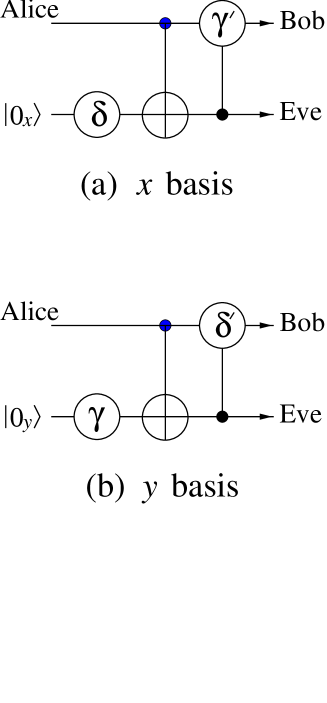
FIG. 3.: Two circuits which produce the same isometry as Fig. 2(a). The circuit in (a) is in the $x$ basis, that in (b) is in the $y$ basis; see text.

In particular, the two circuits shown in Fig. 3 produce the same isometry as those in Fig. 2(a) or (c), when the angles $\gamma^{\prime}$ and $\delta^{\prime}$ are defined to be

$$\gamma^{\prime}=\pi/2-\gamma,\quad\delta^{\prime}=\pi/2-\delta,$$ (51)

and the action of the various gates is understood in the the following way. In Fig. 3(a) the gates are to be thought of as in the $x$ representation using the basis (44). In particular, the controlled-NOT represents the transformation (39), but with $0$ and $1$ replaced everywhere by $0_{x}$ and $1_{x}$, respectively. Likewise, the action of the one-qubit gate represented by $\delta$ inside a circuit is the same as (41) provided $0$ and $1$ are replaced everywhere in (41)—on both sides—with $0_{x}$ and $1_{x}$, and $\phi$ is set equal to $\delta$. Next, the two-qubit gate following the controlled-NOT is a “controlled-rotation” producing the transformation

$$|\alpha\rangle|0_{x}\rangle \rightarrow \left[R(+\gamma^{\prime})|\alpha\rangle\right]\otimes|0_{x}\rangle,$$ (52)

$$|\alpha\rangle|1_{x}\rangle \rightarrow \left[R(-\gamma^{\prime})|\alpha\rangle\right]\otimes|1_{x}\rangle,$$ (53)

where the one qubit gate $R(\phi)$ is (41) in the $x$ representation: $0$ and $1$ replaced by $0_{x}$ and $1_{x}$. Note that the “rotation” on qubit $a$ is carried out in opposite senses depending upon whether $b$ is $|0_{x}\rangle$ or $|1_{x}\rangle$. Also, note that the initial state of the $b$ qubit is $|0_{x}\rangle$, rather than $|0\rangle$, as in Fig. 2.

The circuit in Fig. 3(b) is in the $y$ representation, which means that it is to be interpreted in the same way as (a), but with $0_{y}$ and $1_{y}$ substituted for $0_{x}$ and $1_{x}$. Note that the circuits in Fig. 3 produce an isometry equivalent to Fig. 2 with the definitions for the $x$ and $y$ bases given in (44) and (45), but will not (at least in general) do so for other basis choices using different phases. For example, using $|0_{x}\rangle$ as defined in (44), but replacing $|1_{x}\rangle$ with $(|1\rangle-|0\rangle)/\sqrt{2}$, and then using the circuit in Fig. 3(a) will produce a very different result (try it!).

FIG. 4.: Family of eight quantum histories for the circuit in Fig. 3(a).

Suppose Alice sends a signal using the $x$ mode, and Bob and Eve eventually measure their qubits in the same mode. Whatever two-qubit machine Eve employs (e.g., that of Fig. 2(a)), we can, for purposes of obtaining an intuitive picture of what is going on, imagine that copies are produced by the circuit shown in Fig. 3(a), as this yields the same isometry. This circuit can be analyzed in the same manner as that in [12], using an appropriate family of quantum histories in which every qubit is in either the $|0_{x}\rangle$ or the $|1_{x}\rangle$ state at times when it is not inside one of the gates. The different possible histories of this type are indicated schematically in Fig. 4, where the $x$ subscripts have been omitted. At time $t_{0}$ the two qubits have not passed through any gates, and the two possible initial states, written as $|ab\rangle$, are $|0_{x}0_{x}\rangle$ and $|1_{x}0_{x}\rangle$. At $t_{1}$ the $b$ qubit has passed through the $\delta$ gate, so it can be either $|0_{x}\rangle$ or $|1_{x}\rangle$; the probability of the latter is

$$q_{x}=\left[\sin(\delta/2)\right]^{2}={\textstyle{1\over 2}}(1-\cos\delta).$$ (54)

This probability can be computed in the standard way using weights [13]; note that it is the same as what one would calculate if a measurement on this qubit were to take place at time $t_{1}$ [14]. By time $t_{2}$ the two qubits have passed thought the controlled-NOT gate, while at $t_{3}$ the $a$ qubit has passed through the $\gamma^{\prime}$ gate. In passing through this gate, the $a$ qubit is flipped, from $|0_{x}\rangle$ to $|1_{x}\rangle$, or vice versa, with a probability

$$p_{x}=\left[\sin(\gamma^{\prime}/2)\right]^{2}={\textstyle{1\over 2}}(1-\sin\gamma),$$ (55)

independent of whether the $b$ qubit is in the state $|0_{x}\rangle$ or $|1_{x}\rangle$, since the probability only depends on the magnitude, not the sign of $\gamma^{\prime}$.

The eight histories in Fig. 4 constitute a family of quantum histories which can be treated in the same way as a stochastic family of classical histories, as long as quantum consistency conditions are satisfied [13]. That these conditions are, indeed, satisfied for the family under consideration follows from the fact that the two initial states are mutually orthogonal, and for each initial state, all four final states at the right side of Fig. 4 are mutually orthogonal. Hence the corresponding chain or weight operators are orthogonal.

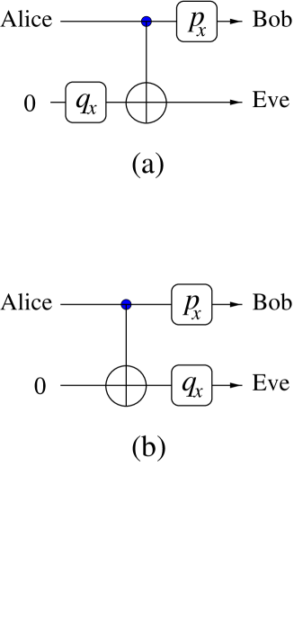
FIG. 5.: Classical stochastic circuits which are equivalent to Fig. 3(a) when using the consistent family of Fig. 4.

Consequently, the action of the circuit in Fig. 3(a) is precisely the same as that of a classical stochastic circuit shown in Fig. 5(a), in which the gates labeled $p_{x}$ and $q_{x}$ correspond to randomly flipping a bit from 0 to 1, or vice versa, with probabilities $p_{x}$ and $q_{x}$. The effect of the $q_{x}$ gate is the same if it is placed after, rather than before, the controlled-NOT, as in Fig. 5(b), which makes the action of the circuit perfectly transparent: Since the $b$ bit is initially 0, the controlled-NOT copies the $a$ bit, 0 or 1, to the $b$ bit. Then both bits are randomly flipped with appropriate probabilities before the $a$ bit is measured by Bob and the $b$ bit by Eve.

It is evident that the eavesdropper will obtain the most information possible when $q_{x}=0$, while $p_{x}=0$ yields the minimum amount of noise in the Alice-to-Bob channel. Thus, choosing $\delta=0$ and $\gamma=\pi/2$ represents the optimal eavesdropping strategy if the $x$ mode is considered by itself. But these values create problems when Alice transmits using the $y$ mode. To analyze what happens in this case, it is convenient to imagine that the actual copying machine, whatever it may be, is replaced by the circuit in Fig. 3(b), which produces the same isometry. Our preceding analysis of part (a) of that figure can be applied to (b) by simply replacing $x$ with $y$ and noting the difference in the gate parameters in the two cases. Thus the consistent family is that of Fig. 4, where one now understands the symbols as having $y$ subscripts, and the action of the quantum circuit, for the $y$ mode, is the same as that of the classical circuits in Fig. 5, with $p_{x}$ and $q_{x}$ replaced by

$$p_{y} = \left[\sin(\delta^{\prime}/2)\right]^{2}={\textstyle{1\over 2}}(1-\sin\delta),$$ (56)

$$q_{y} = \left[\sin(\gamma/2)\right]^{2}={\textstyle{1\over 2}}(1-\cos\gamma).$$ (57)

Consequently, the choice $\delta=0$, which provides Eve with the optimal amount of information about signals in the $x$ mode, creates the maximum possible amount of noise in the Alice-to-Bob channel when used in the $y$ mode. Likewise, if Eve chooses $\gamma=\pi/2$ in order to remain “invisible”, producing no noise, when Alice is transmitting and Bob is measuring in the $x$ mode, the consequence will be that she gains no information at all when Alice transmits in the $y$ mode.

Many other circuits will produce the same isometry on the $a$ qubit as those in Fig. 2(a) and Fig. 3(a) and (b). For example, the two shown in Fig. 6(a) and (b) are similar to those shown in Fig. 3, except that the destination of the final bits has been interchanged. The four circuits in Figs. 3 and 6 represent different unitary transformations, and thus an actual copying machine could employ only one of these circuits. Hence it is worth emphasizing, once again, that all of these circuits, because they yield the same isometry, produce precisely the same result in terms of copies of whatever Alice sends, in the $x$ or $y$ or in any other mode. However, some circuits are more useful than others when one wants to form an intuitive picture of why certain parameter values lead to particular sorts of errors.

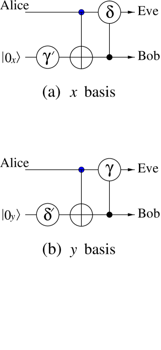
FIG. 6.: A circuit (a) in the $x$ basis and a different circuit (b) in the $y$ basis which produce the same isometry as the circuits in Fig. 2(a), (c), and Fig. 3.

D The B92 cryptographic scheme

In the B92 cryptographic protocol, Alice sends signals through a quantum channel in one of two non-orthogonal states, $|\kappa_{0}\rangle$ and $|\kappa_{1}\rangle$, chosen at random, while Bob makes measurements in one of two orthonormal bases, also chosen at random, one of which includes $|\kappa_{0}\rangle$ and the other $|\kappa_{1}\rangle$. For details, see [7]. Once again, eavesdropping is detected through the production of noise that can be detected by the legitimate users of the channel.

Fuchs and Peres [7] carried out a numerical and analytic study of the problem of distinguishing these two non-orthogonal states, and found an optimal strategy (under certain plausible assumptions) for doing this with minimal disturbance to the original signal, the one sent on to Bob. This strategy can be carried out using the two-qubit copying circuit in Fig. 3(a). Let the two non-orthogonal states used by Alice be

$$|\kappa_{0}\rangle = \cos\bar{\alpha}|0_{x}\rangle+\sin\bar{\alpha}|1_{x}\rangle,$$ (58)

$$|\kappa_{1}\rangle = \sin\bar{\alpha}|0_{x}\rangle+\cos\bar{\alpha}|1_{x}\rangle,$$ (59)

with $\bar{\alpha}$ ($\alpha$ in [7]) a parameter which determines the degree of non-orthogonality. Eve carries out measurements in the $x$ basis $|0_{x}\rangle,|1_{x}\rangle$, and uses this information to try and determine whether Alice transmitted $|\kappa_{0}\rangle$ or $|\kappa_{1}\rangle$.

The copying machine in Fig. 3(a) has two parameters $\delta$ and $\gamma^{\prime}$ which are chosen by Eve in the following way. The value $\delta=0$ provides Eve with copies of the states (59) which are optimal in the sense that her measurements provide the best possible discrimination between them; perfect discrimination is not possible, because $|\kappa_{0}\rangle$ and $|\kappa_{1}\rangle$ are not orthogonal. Choosing some other value of $\delta$ reduces the amount of information that Eve can gain about the transmitted signals. For a given $\delta$, Eve chooses $\gamma^{\prime}$ in such a way as to minimize the noise produced in the Alice-to-Bob circuit. The appropriate value is worked out in [7], where the parameters $\phi$ and $\theta$ are related to our $\delta$ and $\gamma^{\prime}$ by

$$\phi=\delta/2,\quad\theta=\gamma^{\prime}/2.$$ (60)

While the optimal $\gamma^{\prime}$ is a somewhat complicated function of $\delta$, it turns out that by increasing $\delta$ and thereby reducing the amount of information she obtains, Eve can also reduce the amount of noise detectable by Alice and Bob. Thus the optimal strategy can be thought of either as obtaining the most information for a given level of noise, or producing the least amount of noise (by a suitable choice of $\gamma^{\prime}$) for a given amount of information (determined by the choice of $\delta$).

The consistent family of Fig. 4 is inappropriate for analyzing this process because neither Alice nor Bob employ the $|0_{x}\rangle,|1_{x}\rangle$ basis. Nevertheless, because Eve measures her qubit in this basis, there is a consistent quantum-mechanical description in which Eve’s qubit is in one of these two states at all times after it leaves the controlled-NOT gate in Fig. 3(a). Consequently, her measurement reveals a pre-existing value, and the measurement can equally well be carried out before the qubit reaches the controlled-rotation gate, as in the modified circuit in Fig. 7. In this circuit the results of the measurement of $|0_{x}\rangle$ or $|1_{x}\rangle$ are used to produce a “classical” signal which controls the operation of a one qubit gate that carries out a unitary transformation, $R(+\gamma^{\prime})$ or $R(-\gamma^{\prime})$ as appropriate, on the qubit sent on to Bob. This use of retrodiction for simplifying a quantum circuit has been employed previously to simplify the Fourier transform in Shor’s factorization algorithm [15], and to study teleportation [16]. Its justification lies in a correct application of consistent-history methods [13].

FIG. 7.: Improved eavesdropping machine for the B92 protocol, in which the last gate in Fig. 3(a) has been replaced by two single-qubit operations determined by Eve’s measurement result: $R(\gamma^{\prime})$ for $|0_{x}\rangle$ and $R(-\gamma^{\prime})$ for $|1_{x}\rangle$. Note that the gate notations and Eve’s measurement are in the $x$ basis, as in Fig. 3(a).

Since one-qubit gates, even those controlled by classical signals, are likely to be much easier to construct than two qubit gates, the circuit in Fig. 7 represents a cost-effective approach to eavesdropping in the case of the B92 scheme. Unfortunately (or perhaps fortunately), it cannot be used for the BB84 protocol discussed earlier, because in that case Eve does not know ahead of time which mode Alice will employ for transmitting signals, and therefore has to wait until after the copying process is complete before deciding whether to carry out a measurement in the $x$ or the $y$ basis.

VII Summary and open questions

We have carried out a general analysis of a unitary transformation on two qubits from the point of view of a copying machine producing two copies of an arbitrary state of one of the input qubits while the other is held fixed. Such a transformation produces an isometry mapping the input qubit onto a two dimensional subspace ${\cal G}$ of the tensor product ${\cal A}\otimes{\cal B}$ of the two qubits. Central to our analysis is the theorem in Sec. II A according to which there is a basis for ${\cal G}$ in the canonical form given by (6). In some sense this is an extension, to a particular case, of the familiar Schmidt representation for a vector on an arbitrary tensor product ${\cal A}\otimes{\cal B}$. Using this canonical basis allows us to write an arbitrary isometry as a relatively simple canonical isometry, depending on two real parameters, preceded and followed by some additional unitary operations on individual qubits.

A Bloch sphere representation of the output qubits, Sec. III, provides a geometrical picture which is very useful for understanding what sorts of copying errors can occur and the limitations on copy quality imposed by quantum theory. Despite its simplicity (or perhaps because of it), a two-qubit copying machine produces optimal copies according to the criteria worked out in [2]. By using a stochastic generalization, Sec. IV, one can obtain greater flexibility in determining the types of errors which are produced by the machine.

An isometry can be carried out using one of several possible quantum circuits constructed from one-qubit gates and controlled-NOT two-qubit gates, Sec. V. As two-qubit gates are likely to prove rather expensive, it is worth noting that two of them are sufficient, and also necessary for a general isometry. In addition, the canonical isometry corresponding to the canonical basis choice for ${\cal G}$ requires two one-qubit gates, whereas a general isometry requires a total of five one-qubit gates. Some gates controlled by a “classical” stochastic signal are needed to implement a stochastic copying machine.

The two-qubit copier suffices for carrying out the optimal eavesdropping strategy derived in [6] for the BB84 cryptographic scheme. The Bloch sphere picture is particularly valuable in showing why this simpler copier can perform as well as the three-qubit machines proposed in [2, 12]. The stochastic two-qubit copier will also do as well as a three-qubit copier for certain generalizations of BB84. Physical insight into how the parameters of the two-qubit machine determine the information gained by the eavesdropper and the noise produced in the channel between the legitimate users is obtained by employing consistent families of quantum histories in two different circuits producing the same isometry.

A two-qubit copier which carries out the optimal eavesdropping strategy for the B92 cryptographic protocol proposed by Fuchs and Peres [7] can be further simplified by replacing the second controlled-NOT gate by a one-qubit gate controlled by the classical signal produced by an earlier measurement. This trick for producing a more economical machine relies upon the justification of quantum retrodiction provided by a consistent history analysis as first pointed out in [15].

While we have been able to characterize the most general isometry from one qubit to a tensor product space ${\cal A}\otimes{\cal B}$ of two qubits, this is not the same thing as describing the most general unitary transformation on ${\cal A}\otimes{\cal B}$, where work remains to be done [17]. Generalizing the results of this paper to spaces ${\cal A}$ and ${\cal B}$ of dimension greater than two represents a challenging problem. One step towards solving it would be to find some counterpart of the canonical basis, (6), when ${\cal G}$, ${\cal A}$, and ${\cal B}$ are of any dimension. Another would be the development of some geometrical analogy of the Bloch sphere picture for higher-dimensional spaces. And extensions to tensor products of three or more spaces of any of our results would represent a significant contribution to quantum information theory. The possibilities and limitations of stochastic copying machines are worth exploring, given that in certain circumstances they appear to offer a more economical solution to copying problems than employing additional ancillary qubits in a quantum circuit.

A The canonical representation

Given a state $|\psi\rangle$ of ${\cal A}\otimes{\cal B}$ in the form

$$|\psi\rangle=\sum_{jk}\tau_{jk}|a^{\prime}_{j}b^{\prime}_{k}\rangle,$$ (A1)

where $\{|a^{\prime}_{0}\rangle,|a^{\prime}_{1}\rangle\}$ and $\{|b^{\prime}_{0}\rangle,|b^{\prime}_{1}\rangle\}$ are any orthonormal bases of ${\cal A}$ and ${\cal B}$, it is easy to show that a necessary and sufficient condition for $|\psi\rangle$ to be a product state of the form $|a\rangle\otimes|b\rangle$ is that

$$\tau_{00}\tau_{11}=\tau_{01}\tau_{10}.$$ (A2)

The lemma that a two-dimensional subspace ${\cal G}$ of ${\cal A}\otimes{\cal B}$ always contains a non-zero product state can be established as follows. Assume that $|\psi^{\prime}\rangle$ and $|\psi^{\prime\prime}\rangle$ are linearly independent vectors in ${\cal G}$, and $|\psi^{\prime}\rangle$ is not a product state. Applying the condition (A2) to

$$|\psi\rangle=\lambda|\psi^{\prime}\rangle+|\psi^{\prime\prime}\rangle=\sum_{jk}(\lambda\tau^{\prime}_{jk}+\tau^{\prime\prime}_{jk})|a^{\prime}_{j}b^{\prime}_{k}\rangle$$ (A3)

leads to a quadratic equation in $\lambda$ with a non-zero coefficient of $\lambda^{2}$, which thus has at least one root corresponding to a product state. (In general one expects two roots and two linearly-independent product states.) Consequently, there is an orthonormal basis

$$|\bar{g}_{0}\rangle=|\bar{a}_{0}\bar{b}_{0}\rangle,\quad|\bar{g}_{1}\rangle=c_{01}|\bar{a}_{0}\bar{b}_{1}\rangle+c_{10}|\bar{a}_{1}\bar{b}_{0}\rangle+c_{11}|\bar{a}_{1}\bar{b}_{1}\rangle$$ (A4)

of ${\cal G}$ written in terms of suitable orthonormal bases $\{|\bar{a}_{j}\rangle\}$ and $\{|\bar{b}_{j}\rangle\}$ of ${\cal A}$ and ${\cal B}$, where $|\bar{g}_{0}\rangle$ is the product state whose existence is guaranteed by the lemma. If $c_{11}=0$, removing the bars in (A4) yields (6) with $\bar{\mu}=0$, and our task is finished.

Thus from now on we assume that

$$c_{11}\neq 0.$$ (A5)

There is then a second product state

$$|\psi\rangle=(c_{01}c_{10}/c_{11})|\bar{g}_{0}\rangle+|\bar{g}_{1}\rangle,$$ (A6)

in ${\cal G}$—as can be verified using (A2)—which is linearly independent of $|\bar{g}_{0}\rangle$. It is convenient to write these two linearly-independent product states in the normalized (but not orthogonal) form

$$|\pi_{j}\rangle=|\alpha_{j}\rangle\otimes|\beta_{j}\rangle,$$ (A7)

for $j=0,1$, with

$$\langle\alpha_{j}|\alpha_{j}\rangle=1=\langle\beta_{j}|\beta_{j}\rangle,$$ (A8)

and with phases chosen so that

$$0\leq\langle\alpha_{0}|\alpha_{1}\rangle<1,\quad 0\leq\langle\beta_{0}|\beta_{1}\rangle<1.$$ (A9)

The inequalities in (A9) are strict, since were it the case, for example that, $\langle\alpha_{0}|\alpha_{1}\rangle=1$, this would mean $|\alpha_{0}\rangle=|\alpha_{1}\rangle$, and ${\cal G}$ would consist entirely of product states of the form $|\alpha_{0}\rangle\otimes|b\rangle$, which is inconsistent with (A5).

Because of the strict inequality just noted, none of the four kets

$$|\hat{a}_{0}\rangle=|\alpha_{0}\rangle+|\alpha_{1}\rangle,\quad|\hat{a}_{1}\rangle=|\alpha_{0}\rangle-|\alpha_{1}\rangle,$$ (A10)

$$|\hat{b}_{0}\rangle=|\beta_{0}\rangle+|\beta_{1}\rangle,\quad|\hat{b}_{1}\rangle=|\beta_{0}\rangle-|\beta_{1}\rangle$$ (A11)

is zero, and since each pair is orthogonal,

$$\langle\hat{a}_{0}|\hat{a}_{1}\rangle=0=\langle\hat{b}_{0}|\hat{b}_{1}\rangle,$$ (A12)

one can construct orthonormal bases for ${\cal A}$ and ${\cal B}$ by appropriate normalization:

$$|a_{j}\rangle=|\hat{a}_{j}\rangle/\sqrt{\langle a_{j}|a_{j}\rangle},\quad|b_{j}\rangle=|\hat{b}_{j}\rangle/\sqrt{\langle b_{j}|b_{j}\rangle}.$$ (A13)

Inverting the relations (A11) allows one to write

$$|\alpha_{0}\rangle=\kappa|a_{0}\rangle+\bar{\kappa}|a_{1}\rangle,\quad|\alpha_{1}\rangle=\kappa|a_{0}\rangle-\bar{\kappa}|a_{1}\rangle,$$ (A14)

$$|\beta_{0}\rangle=\lambda|b_{0}\rangle+\bar{\lambda}|b_{1}\rangle,\quad|\beta_{1}\rangle=\lambda|b_{0}\rangle-\bar{\lambda}|b_{1}\rangle,$$ (A15)

where the constants $\kappa,\bar{\kappa},\lambda,\bar{\lambda}$ are all strictly positive numbers. Consequently, the two orthogonal vectors

$$|\hat{g}_{0}\rangle=|\pi_{0}\rangle+|\pi_{1}\rangle=2(\kappa\lambda|a_{0}b_{0}\rangle+\bar{\kappa}\bar{\lambda}|a_{1}b_{1}\rangle),$$ (A16)

$$|\hat{g}_{1}\rangle=|\pi_{0}\rangle-|\pi_{1}\rangle=2(\kappa\bar{\lambda}|a_{0}b_{1}\rangle+\bar{\kappa}\lambda|a_{1}b_{0}\rangle),$$ (A17)

when appropriately normalized, provide an orthonormal basis for ${\cal G}$ in the form (6).

B Symmetries of coefficients in the canonical representation

The representation (6) is in general not unique in that the same subspace ${\cal G}$ may possess an alternative orthonormal basis

$$|g^{\prime}_{0}\rangle = \mu^{\prime}|a^{\prime}_{0}b^{\prime}_{0}\rangle+\bar{\mu}^{\prime}|a^{\prime}_{1}b^{\prime}_{1}\rangle,$$ (B1)

$$|g^{\prime}_{1}\rangle = \nu^{\prime}|a^{\prime}_{0}b^{\prime}_{1}\rangle+\bar{\nu}^{\prime}|a^{\prime}_{1}b^{\prime}_{0}\rangle,$$ (B2)

written using alternative orthonormal bases $\{|a^{\prime}_{0}\rangle,|a^{\prime}_{1}\rangle\}$ for ${\cal A}$ and $\{|b^{\prime}_{0}\rangle,|b^{\prime}_{1}\rangle\}$ for ${\cal B}$. Different sets of coefficients $\{\mu^{\prime},\bar{\mu}^{\prime},\nu^{\prime},\bar{\nu}^{\prime}\}$ which can be used to represent the same subspace will be called equivalent, and maps which carry one set of coefficients to an equivalent set will be referred to as symmetry operations. (Note that replacing the coefficients in (6) by an equivalent set while leaving the bases for ${\cal A}$ and ${\cal B}$ unchanged will, in general, lead to a different subspace ${\cal G}$; the coefficient change must be accompanied by changes in the bases if ${\cal G}$ is to remain unaltered.)

It is easy to show that multiplying the coefficients by arbitrary phase factors,

$$\mu^{\prime}=e^{i\phi_{00}}\mu,\quad\bar{\mu}^{\prime}=e^{i\phi_{11}}\bar{\mu},\quad\nu^{\prime}=e^{i\phi_{01}}\nu,\quad\bar{\nu}^{\prime}=e^{i\phi_{10}}\bar{\nu},$$ (B3)

for any choice of $\phi_{jk}$, is a symmetry operation in the sense just defined: insert

$$|a^{\prime}_{j}\rangle=e^{i\alpha_{j}}|a_{j}\rangle,\quad|b^{\prime}_{j}\rangle=e^{i\beta_{j}}|b_{j}\rangle,\quad|g^{\prime}_{j}\rangle=e^{i\gamma_{j}}|g_{j}\rangle,$$ (B4)

in (B2) and choose the six phases $\alpha_{0},\alpha_{1},\beta_{0},\beta_{1},\gamma_{0},\gamma_{1}$ so as to recover (6). (This is an alternative demonstration that the coefficients in (6) can always be chosen to be real and positive.)

Additional symmetries arise because it does not matter which of the special basis vectors in ${\cal G}$ is called $|g_{0}\rangle$ and which $|g_{1}\rangle$; likewise, one can interchange $|a_{0}\rangle$ with $|a_{1}\rangle$, or $|b_{0}\rangle$ with $|b_{1}\rangle$. These interchanges give rise to three symmetry operations on the coefficients in addition to those in (B3): (i) interchange $\mu$ with $\nu$, and $\bar{\mu}$ with $\bar{\nu}$; (ii) interchange $\mu$ with $\bar{\mu}$, and $\nu$ with $\bar{\nu}$; (iii) interchange $\mu$ with $\bar{\nu}$, and $\nu$ with $\bar{\mu}$. Of course, (iii) is just the product of (i) and (ii). (Note that interchanging $\mu$ with $\bar{\mu}$ while keeping $\nu$ and $\bar{\nu}$ fixed is not a symmetry operation.)

When applied to the trigonometric representation (9), these symmetry operations allow one to (i) change the sign of $\zeta$; (ii) change the sign of $\eta$; (iii) increase both $\zeta$ and $\eta$ by $\pi$; (iv) interchange $\zeta$ with $\eta$. (Note that increasing $\zeta$ by $\pi$ without changing $\eta$ is not a symmetry operation, although either $\zeta$ or $\eta$ can be increased by $2\pi$ while the other remains fixed.) Combinations of these operations map any $(\zeta,\eta)$ in the square

$$0\leq\zeta\leq\pi,\quad 0\leq\eta\leq\pi,$$ (B5)

corresponding to positive coefficients in (9), onto the equivalent points

$$(\eta,\zeta),\quad(\pi-\zeta,\pi-\eta),\quad(\pi-\eta,\pi-\zeta),$$ (B6)

from which it follows that $(\zeta,\eta)$ can always, if desired, be chosen to lie in the region (10).

C Finding the canonical basis

The construction in App. A which demonstrates the existence of the canonical representation is not an easy way to find it. The following is an alternative approach which is simpler and works except for certain degenerate cases. In particular, it does not require that one find product states in ${\cal G}$.

Given two linearly independent vectors in ${\cal G}$, one can construct (Gram-Schmidt) an orthonormal basis $\{|\bar{g}_{0}\rangle,|\bar{g}_{1}\rangle\}$, and from it the (unique) projector

$$G=|\bar{g}_{0}\rangle\langle\bar{g}_{0}|+|\bar{g}_{1}\rangle\langle\bar{g}_{1}|=|g_{0}\rangle\langle g_{0}|+|g_{1}\rangle\langle g_{1}|$$ (C1)

onto the subspace ${\cal G}$, along with its partial traces

$$G_{A} = {\rm Tr}_{{\cal B}}[G]=(\mu^{2}+\nu^{2})|a_{0}\rangle\langle a_{0}|+(\bar{\mu}^{2}+\bar{\nu}^{2})|a_{1}\rangle\langle a_{1}|,$$ (C2)

$$G_{B} = {\rm Tr}_{{\cal A}}[G]=(\mu^{2}+\bar{\nu}^{2})|b_{0}\rangle\langle b_{0}|+(\bar{\mu}^{2}+\nu^{2})|b_{1}\rangle\langle b_{1}|,$$ (C3)

which are operators on ${\cal A}$ and ${\cal B}$, respectively. Here we are assuming, for convenience, that the coefficients in (6) are real and positive.

If the eigenvalues of $G_{A}$, in parentheses on the right side of (C3), are non-degenerate, the dyads $|a_{0}\rangle\langle a_{0}|$ and $|a_{1}\rangle\langle a_{1}|$ are uniquely defined up to identifying which is which. We can, for example, assume that $|a_{0}\rangle\langle a_{0}|$ corresponds to the larger and $|a_{1}\rangle\langle a_{1}|$ to the smaller eigenvalue. A similar comment applies when the eigenvalues of $G_{B}$ in (C3) are non-degenerate. The eigenvalues of $G_{A}$ and $G_{B}$, along with the normalization condition (7), serve to determine the non-negative coefficients $\mu,\bar{\mu},\nu,$ and $\bar{\nu}$.

The dyads $|a_{0}\rangle\langle a_{0}|$, etc., in (C3) determine vectors $|a^{\prime}_{0}\rangle$, $|a^{\prime}_{1}\rangle$, $|b^{\prime}_{0}\rangle$, and $|b^{\prime}_{1}\rangle$ which are identical to their unprimed counterparts in (6) apart from the arbitrary phase factors in (B4). These phases cannot be chosen arbitrarily, because the relative phases of the summands on the right side of (6) is significant, and the information in the partial traces (C3) is not enough to determine them, so an additional step is needed.

If $|g\rangle$ is any vector in ${\cal G}$ (and hence a linear combination of $|g_{0}\rangle$ and $|g_{1}\rangle$) such that both $\langle g|a_{0}b_{0}\rangle$ and $\langle g|a_{1}b_{1}\rangle$ are nonzero, then the positivity of the coefficients in (6) implies that

$${\rm Ph}(\langle g|a_{0}b_{0}\rangle)={\rm Ph}(\langle g|a_{1}b_{1}\rangle),$$ (C4)

where the phase ${\rm Ph}(z)$ is $\phi$ when $z=|z|e^{i\phi}$. Given such a $|g\rangle$, which could be $|\bar{g}_{0}\rangle$ or $|\bar{g}_{1}\rangle$, the phases of the inner products $\langle g|a^{\prime}_{0}b^{\prime}_{0}\rangle$ and $\langle g|a^{\prime}_{1}b^{\prime}_{1}\rangle$, along with (C4), constrain the choices of $\alpha_{j}$ and $\beta_{j}$ in (B4). The requirement that

$${\rm Ph}(\langle g|a_{0}b_{1}\rangle)={\rm Ph}(\langle g|a_{1}b_{0}\rangle),$$ (C5)

again based on (6), applied to a non-vanishing pair of inner products $\langle g|a^{\prime}_{0}b^{\prime}_{1}\rangle$ and $\langle g|a^{\prime}_{1}b^{\prime}_{0}\rangle$, (with the same or a different $|g\rangle$ from that in (C4)) yields a second constraint for the $\alpha_{j}$ and $\beta_{j}$. When both constraints are satisfied, the remaining freedom in choosing phases simply determines the overall phases of $|g_{0}\rangle$ and $|g_{1}\rangle$.

REFERENCES

- [1] W. K. Wootters and W. H. Zurek, Nature 299, 802 (1982).
- [2] C.-S. Niu and R. B. Griffiths, Phys. Rev. A (to appear), quant-ph/9805073.
- [3] D. Bruß, D. P. DiVincenzo, A. Ekert, C. A. Fuchs, C. Macchiavello, and J. A. Smolin, Phys. Rev. A 57, 2368 (1998).
- [4] C. Bennett and G. Brassard, Proceedings of the IEEE International Conference on Computer, System, and Signal Processing, Bangalore, India (IEEE, New York, 1984), p. 175.
- [5] C. Bennett, Phys. Rev. Lett. 68, 3121 (1992).
- [6] C. Fuchs, N. Gisin, R. B. Griffiths, C.-S. Niu, and A. Peres, Phys. Rev. A 56, 1163 (1997).
- [7] C. Fuchs and A. Peres, Phys. Rev. A 53, 2038 (1996).
- [8] C. A. Fuchs, Fortschr. Phys. 46, 535 (1998).
- [9] The idea for a stochastic copier was suggested to us by N. Gisin, private communication.
- [10] A. Barenco et al., Phys. Rev. A 52, 3457 (1995).
- [11] For an introduction to the subject, see C. Bennett, G. Brassard, and A. Ekert, Scientific American, Oct. 1992, p. 50, and R. J. Hughes, D. M. Alde, P. Dyer, G. G. Luther, G. L. Morgan, and M. Schauer, Contemporary Physics 36, 149 (1995).
- [12] R. B. Griffiths and C.-S. Niu, Phys. Rev. A 56, 1173 (1997).
- [13] R. B. Griffiths, Phys. Rev. A 54, 2759 (1996).
- [14] While imagining that a measurement takes place can be an aid to carrying out a calculation of the desired probability, it should be emphasized that the probability is valid in the absence of any measurement provided the consistency conditions for the family of histories are fulfilled.
- [15] R. B. Griffiths and C.-S. Niu, Phys. Rev. Lett. 76, 3228 (1996).
- [16] G. Brassard, S. L. Braunstein, and R. Cleve, Physica D (to appear).
- [17] D. DiVincenzo, private communication.