Long-time dynamics of spontaneous parametric down-conversion and quantum limitations of conversion efficiency

Abstract

We analyze the long-time quantum dynamics of degenerate parametric down-conversion from an initial sub-harmonic vacuum (spontaenous down-conversion). Standard linearization of the Heisenberg equations of motions fails in this case, since it is based on an expansion around an unstable classical solution and neglects pump depletion. Introducing a mean-field approximation we find a periodic exchange of energy between the pump and subharmonic mode goverened by an anharmonic pendulum equation. From this equation the optimum interaction time or crystal length for maximum conversion can be determined. A numerical integration of the 2-mode Schrödinger equation using a dynamically optimized basis of displaced and squeezed number states verifies the characteristic times predicted by the mean-field approximation. In contrast to semiclassical and mean-field predictions it is found that quantum fluctuations of the pump mode lead to a substantial limitation of the efficiency of parametric down-conversion.

I introduction

Owing to its relative simplicity but yet richness, the process of parametric down-conversion is one of the most intensively studied in quantum optics [1, 2, 3, 4, 5]. Here photons of a coherent pump field are transformed into pairs of signal and idler photons [6, 7] which can display nonclassical quantum correlations [8] or perfect squeezing in the case of degeneracy. We here restrict ourselves to the latter situation, where both down-converted photons are emitted into the same radiation mode. A standard approach to analyze the quantum fluctuation in nonlinear optical system is to assume small fluctuations around the classical solutions, i.e. to linearize the Heisenberg equations of motion . The linearization approximation fails however in the case of a vacuum input of the sub-harmonic mode, since it neglects pump depletion and is thus only valid for an infinite input intensity of the pump field. Thus linearization can neither be used to study the effect of finite system size, i.e. finite pump intensity nor the long-time dynamics of the parametric process.

Using a short-time perturbation expansion, Crouch and Braunstein analyzed the leading order corrections to the maximum degree of squeezing due to finite pump intensities [9]. Here we are interested in the long-time behaviour of parametric down-conversion. In particular we aim to determine the optimum interaction time (propagation length in the crystal) for maximum down-conversion and the maximum efficiency of this process. In the case of a vacuum input of the sub-harmonic mode, both quantities are goverened by quantum effects. We find that in contrast to the classical predictions, these quantum effects limit the maximum conversion efficiency from a pump photon into two sub-harmonic photons to a value much less than unity. This limitation could be of importance for applications in quantum communication and cryptography on the single photon level.

II model, classical dynamics and linearisation

In order to describe stationary parametric conversion of travelling-wave pump radiation into travelling-wave sub-harmonic radiation we introduce a moving coordinate system. Ignoring transversal degrees of freedom we find the following Heisenberg equations of motion

$$\frac{\rm d}{{\rm d}t}a_{1} = K\,a_{2}a_{1}^{\dagger},$$ (1)

$$\frac{\rm d}{{\rm d}t}a_{2} = -\frac{K^{*}}{2}a_{1}^{2}.$$ (2)

$a_{1}$ and $a_{2}$ are the bosonic mode operators of the sub-hamonic and pump fields respectively. $K$ describes the strength of the nonlinear process. It is proportional to the nonlinear susceptibility $\chi^{(3)}$ of the crystal and the inverse of the beam diameter. The time evolution in the moving frame corresponds to a spatial evolution in the lab frame and the fields at $t=0$ are the input fields. Due to the phase symmetry of the equations

$$a_{1} \to \pm a_{1}\,{\rm e}^{i\phi_{1}},$$ (3)

$$a_{2} \to \enspace a_{2}\,{\rm e}^{i\phi_{2}},$$ (4)

$$K \to \enspace K\,{\rm e}^{i(2\phi_{1}-\phi_{2})}$$ (5)

we may choose $K$ and the initial amplitude of the pump field $\langle a_{2}(t=0)\rangle$ real. The equations of motion (1,2) obey the Manley-Rowe relation [6, 7], which states that the total energy of the free (!) system is conserved.

$$\frac{\rm d}{{\rm d}t}\langle a_{1}^{\dagger}a_{1}\rangle+2\frac{\rm d}{{\rm d}t}\langle a_{2}^{\dagger}a_{2}\rangle=0.$$ (6)

Even though Eqs.(1) and (2) seem simple, the nonlinearity prevents an analytic solution of the quantum problem. Therefore approximations are necessary. A frequently used approximation is the linearisation around the classical solutions. In order to discuss the validity of this approximation, let us first consider the classical problem, where the Bose operators $a_{1}$ and $a_{2}$ are replaced by c-numbers $\alpha_{1}$ and $\alpha_{2}$.

$$\frac{\rm d}{{\rm d}t}\alpha_{1} = K\,\alpha_{2}\alpha_{1}^{*},$$ (7)

$$\frac{\rm d}{{\rm d}t}\alpha_{2} = -\frac{K}{2}\alpha_{1}^{2}.$$ (8)

One clearly sees, that for vanishing sub-harmonic input, i.e. $\alpha_{1}(0)=0$, both amplitudes remain constant. This solution is linearly unstable and any fluctuation will be exponentially amplified. The time evolution critically depends on the amplitude and phase of an initial classical fluctuation. Thus a classical calculation cannot determine the optimum interaction time (or crystal length) for maximum conversion.

In the standard linearization approach, the pump-mode operator is replaced by its classical input amplitude. This turns the quantum problem into a linear one, which can immediately be solved. One finds that the time-evolution operator of the sub-harmonic mode is given by

$${\sf U}_{\rm lin}(t)={\sf S}[\eta(t)],$$ (9)

where S is the so-called squeezing operator [11]

$${\sf S}[\eta]=\exp\Bigl{\{}\frac{\eta}{2}a_{1}^{\dagger 2}-\frac{\eta^{*}}{2}a_{1}^{2}\Bigr{\}}$$ (10)

with a squeezing parameter that grows linear with time

$$\eta(t)=K\alpha_{2}t.$$ (11)

Since $K$ and $\alpha_{2}$ have been choosen real, the time evolution will lead to a squeezing of the fluctuations of the out-of-phase component of the sub-harmonic mode $p_{1}$, ($a_{1}=x_{1}+ip_{1}$) below the standard vacuum limit. The quantum noise of $p_{1}$ monotonously decreases with time and simultaneously the quantum noise of $x_{1}$ increases. The increase of the fluctuations in the in-phase component $x_{1}$ is associated with a steady increase of the sub-harmonic photon number

$$\langle a_{1}^{\dagger}a_{1}\rangle=\sinh^{2}\eta(t)=\sinh^{2}K\alpha_{2}t.$$ (12)

This result violates the Manley Rowe relations (6) and indicates the breakdown of the linearization for larger times. The growing fluctuations of the (anti-squeezed component of the) sub-harmonic mode can at some point not assumed to be small anymore. They will lead to a decrease (depletion) of the pump-mode amplitude and to fluctuations in this mode.

III mean-field approximation and optimum interaction time

As noted above a linearization of the Heisenberg equations of motion cannot be used to study the long-time behaviour of spontaneous (vacuum input) parametric down-conversion. The quantum fluctuations of the sub-harmonic mode and their backaction onto the pump mode are essential and need to be taken into account. We may however replace the pump-mode amplitude by its average value, which amounts to a mean-field approximation [12]. With this we obtain the equations of motion

$$\frac{\rm d}{{\rm d}t}a_{1} = K\,\langle a_{2}\rangle a_{1}^{\dagger},$$ (13)

$$\frac{\rm d}{{\rm d}t}\langle a_{2}\rangle = -\frac{K^{*}}{2}\langle a_{1}^{2}\rangle.$$ (14)

Thus we have transformed the original set of nonlinear operator equations into a linear operator equation plus a nonlinear classical one. One easily verifies that equations (13) and (14) obey the Manley-Rowe relation.

$$\frac{\rm d}{{\rm d}t}\langle a_{1}^{\dagger}a_{1}\rangle=K\langle a_{2}^{\dagger}\rangle\langle a_{1}^{2}\rangle+c.c.=-2\frac{\rm d}{{\rm d}t}\langle a_{2}^{\dagger}a_{2}\rangle.$$ (15)

The mean-field equations correpond to a time-evolution operator

$${\sf U}_{\rm mf}(t)={\sf D}_{2}\bigl{[}\beta(t)\bigr{]}\,{\sf S}_{1}\bigl{[}\eta(t)\bigr{]},$$ (16)

that consists of a coherent displacement operator for the pump mode and a squeezing operator for the sub-harmonic mode.

$${\sf D}(\alpha) = \exp\bigl{\{}\alpha a^{\dagger}-\alpha^{*}a\bigr{\}},$$ (17)

$${\sf S}(\eta) = \exp\Bigl{\{}\frac{\eta}{2}a^{\dagger 2}-\frac{\eta^{*}}{2}a^{2}\Bigr{\}}.$$ (18)

Thus the interaction leads to a shift of the coherent amplitude of the pump mode by the amount

$$\beta(t)=-\frac{1}{2}K\int_{0}^{t}\!\!\!{\rm d}t^{\prime}\,\langle a_{1}^{2}(t^{\prime})\rangle.$$ (19)

At the same time the sub-harmonic mode is squeezed by

$$\eta(t)=K\int_{0}^{t}\!\!\!{\rm d}t^{\prime}\,\langle a_{2}(t^{\prime})\rangle.$$ (20)

In contrast to the linearisation, the squeezing parameter does not increase indefinitely, since the pump mode amplitude decreases, characterized by the displacement parameter $\beta$. $\beta(t)$ and $\eta(t)$ are not independent. From the mean-field equations we find

$$\ddot{\eta}(t)=K\dot{\beta}(t).$$ (21)

If we know $\eta(t)$ we can immediately obtain the amplitude of the (classical) pump mode from Eq.(20). On the other hand we find the following coupled equations for the sub-harmonic photon number and correlation function

$$\frac{\rm d}{{\rm d}t}\langle a_{1}^{\dagger}a_{1}\rangle = 2\dot{\eta}\,\langle a_{1}a_{1}\rangle,$$ (22)

$$\frac{\rm d}{{\rm d}t}\langle a_{1}a_{1}\rangle = \dot{\eta}\,\Bigl{(}2\langle a_{1}^{\dagger}a_{1}\rangle+1\Bigr{)},$$ (23)

which have the solutions

$$\langle a_{1}^{\dagger}a_{1}\rangle = \sinh^{2}\eta,$$ (24)

$$\langle a_{1}a_{1}\rangle = \frac{1}{2}\sinh 2\eta.$$ (25)

Thus the knowledge of $\eta$ is sufficient to determine all relevant quantities. From (19) and (21) we find $\ddot{\eta}=-(K^{2}/2)\langle a_{1}^{2}\rangle$ and thus the dynamics of the squeezing parameters is goverened by an anharmonic pendulum equation.

$$\ddot{\eta}(t)=-\frac{1}{4}K^{2}\sinh 2\eta(t),$$ (26)

with the initial conditions

$$\eta(0) = 0,$$ (27)

$$\dot{\eta}(0) = K\langle a_{2}(0)\rangle.$$ (28)

The anharmonic pendulum equation with the given initial conditions is equivalent to the integrated Manley-Rowe relation

$$\frac{2}{K^{2}}\dot{\eta}^{2}+\sinh^{2}\eta=2n_{2}^{0}=2|\langle a_{2}(0)\rangle|^{2}.$$ (29)

This suggests a mechnical analogue. If $\eta$ is interpreted as the spatial coordinate of a classical particle moving in one dimension, the first term in Eq.(29) represents its kinetic and the second its potential energy. In the chosen units the kinetic energy is then twice the pump-mode photon number and the potential energy the photon number of the sub-harmonic mode.

FIG. 1.: Squeezing parameter as function of scaled time for coherent pump with input intensity $\langle a_{2}(0)\rangle^{2}=n_{2}^{0}$.

Fig. 1 shows the squeezing parameter as function of the scaled time $K\langle a_{2}(0)\rangle t$ for different initial photon numbers $n_{2}^{0}:=|\langle a_{2}(0)\rangle|^{2}$. The squeezing parameter reaches a maximum value and there is an optimum interaction time or crystal length for maximum squeezing. The corresponding optimum time is a quarter of the oscillation period in the anharmonic potential.

$$KT_{\rm sq}=\frac{1}{2}\int_{0}^{y_{\rm max}}\!\!\!\frac{{\rm d}y}{\sqrt{n_{2}^{0}-\frac{1}{2}\sinh^{2}y}}\approx\frac{1}{4}\,{\rm ln}\,\Bigl{[}n_{2}^{0}\Bigr{]},$$ (30)

where $\sinh^{2}y_{\rm max}=2n_{2}^{0}$. This results agrees with that of the short-time perturbation expansion by Crouch and Braunstein [9]. A comparision with the Crouch-Braunstein result shows however that the maximum amount of noise reduction found in mean-field approximation

$$\langle\Delta p_{1}^{2}\rangle_{\rm min}=\frac{1}{32n_{2}^{0}}$$ (31)

is too small. The mean-field approach neglects the fluctuations of the pump mode, in particular its phase noise. When this is taken into account the minimum fluctuations are only $\langle\Delta p_{1}^{2}\rangle_{\rm min}=1/8\sqrt{n_{2}^{0}}$ [9, 10].

Maximum conversion of pump into sub-harmonic photons is achieved when $\dot{\eta}=0$, i.e. at the turning points of the classical pendulum motion. Thus the optimum conversion time $T_{\rm conv}$ or equivalently the optimum crystal length is determined by

$$K\,T_{\rm conv}=\int_{0}^{y_{\rm max}}\!\!\!\frac{{\rm d}y}{\sqrt{n_{2}^{0}-\frac{1}{2}\sinh^{2}y}}\approx\frac{1}{2}\,{\rm ln}\,\Bigl{[}n_{2}^{0}\Bigr{]},$$ (32)

which is twice the time of maximum squeezing. Fig. 2 shows the scaled photon numbers of the pump and sub-harmonic mode as a function of time.

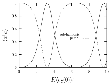
FIG. 2.: Scaled mean photon number of pump (dashed) and sub-harmonic mode (line) as function of scaled time for $\langle a_{2}(0)\rangle=\sqrt{20}$

Since the mean-field approach takes into account the energy transfer from the pump mode into sub-harmonic fluctuations, it correctly describes the oscillatory energy exchange in parametric down-conversion from an initial sub-harmonic vacuum. This is in contrast to the classical or linearization approximation. The mean-field approximation also allows to determine the optimum interaction time for large squeezing or best down-conversion, Eqs.(30,32). The maximum conversion efficiency is unity.

The underlying assumption of the mean-field approach is a quasi-classical description of the pump field. This assumption becomes however questionable at the point of total energy conversion and thus the maximum conversion efficiency obtained in mean-field approximation may not be correct. To calculate this quantity and to discuss the influence of quantum fluctuation in particular of the pump mode we shall numerically integrate the two-mode Schrödinger equation in the next section.

IV numerical integration of two-mode Schrödinger equation and quantum limit to the conversion efficiency

A direct numerical integration of the Schrödinger or Liouville equation is not a straight forward task for multi-mode problems. Unless the interacting modes contain only very few photons, the standard Fock-basis expansion requires the use of a large basis set. For the present problem a large basis set is required in both modes since during the interaction all or almost all photons of the pump mode are converted into sub-harmonic photons and vice versa.

To avoid the large-memory requirement of a simple Fock space expansion one may think of choosing a modified basis adapted to the problem. For example in the initial phase of the process the pump mode is in a coherent state $|\alpha_{2}^{0}\rangle$. Its photon number distribution is Poissonian and thus the required number of basis states is of the order of $|\alpha_{2}^{0}|$, which can be large. On the other hand one can displace the number state basis with the unitary transformation ${\sf D}(\alpha)$ introducing the states

$$|\alpha,n\rangle={\sf D}(\alpha)|n\rangle$$ (33)

which form a complete set. Clearly at $t=0$ only a single state is needed to describe the pump mode if $\alpha=\alpha_{2}^{0}$. As known from the mean-field approach, the coherent amplitude of the pump mode decreases during the interaction and the basis set (33) would soon become ineffective. Thus the parameter $\alpha$ needs to be dynamically adapted, $\alpha\to\alpha(t)$. This is easy to implement in a numerical algorithm that solves the differential equation. In each time step the expansion coefficients are calculated in an adapted basis which uses parameters obtained in the previous time step. These coefficients are then used to update the basis and so on.

If there is no initial symmetry-breaking the coherent amplitude of the subharmonic mode remains zero at all times. Thus a dynamically adapted coherent displacement of the sub-harmonic basis states is not useful. However we have seen in the previous section that the time evolution of this mode is approximately described by a dynamical squeezing ${\sf S}(\eta)$, see Eq.(16). Therefore we expand the state vector of the sub-harmonic mode in a squeezed number-basis

$$|\eta,n\rangle={\sf S}(\eta)\,|n\rangle,$$ (34)

with a dynamically adapted parameter $\eta=\eta(t)$.

The use of a dynamically optimized squeezed and displaced number basis [12] allowed a numerical integration of the two-mode Schrödinger equation for input photon numbers up to several thousands. In Fig. 3 we have shown the scaled real part of the pump mode amplitude $(\langle a_{2}\rangle=x_{2}+ip_{2})$ and its fluctuations as a function of the scaled time $\tau=K\langle a_{2}(0)\rangle t$. Also shown is the mean-field result. One recognizes good agreement of the predictions for the optimum conversion time from both approaches.

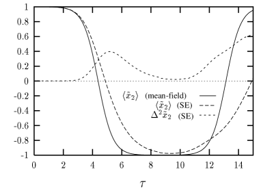
FIG. 3.: Scaled in-phase average quadrature component of pump mode $\langle\tilde{x}_{2}\rangle=\langle x_{2}\rangle/\langle x_{2}(0)\rangle$ from mean-field approximation (line) and numerical integration of two-mode Schrödinger equation (long dashes). Also shown are the fluctuations of $\tilde{x}_{2}$ obtained from numerical integration (short dashes). $\tau=K\langle a_{2}(0)\rangle t$, $\langle a_{2}(0)\rangle=\sqrt{200}$

On the other hand, the numerical solution shows, that at the point of vanishing coherent amplitude of the pump mode, its fluctuations become large. This implies that the coherent-state approximation used in the mean-field approach is not valid near the point of maximum conversion. Furthermore, although the coherent amplitude vanishes, the mean photon number of the pump remains finite and thus the conversion efficiency is less than unity. Fig. 4 illustrates this.

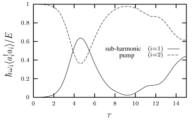
FIG. 4.: Time evolution of energy of pump (dashed) and sub-harmonic mode (line) as function of scaled time $\tau=K\langle a_{2}(0)\rangle t$ for $\langle a_{2}(0)\rangle=\sqrt{200}$.

Shown are the energies of both fields as a function of time. One recognizes a maximum conversion of only about 65% for 200 input photons of the pump mode. Our calculations indicate that this value does not increase with increasing input photon number and is thus not a finite-size effect. Near the point of maximum conversion the pump-mode amplitude becomes small and the back-action of the quantum fluctuations of the sub-harmonic mode (more precisely that of the anti-squeezed quadrature component) onto the pump mode gain importance. They lead to an increase of the in-phase quadrature fluctuations of the pump field and thus a finite amount of energy remains in this mode even though the coherent amplitude vanishes.

V summary

We have analysed the long-time quantum dynamics of degenerate parametric down conversion, for which standard approaches like the linearization of the Heisenberg equations of motion fail. In a mean-field approach, which assumes a coherent pump mode but takes the sub-harmonic fluctions fully into account, an oscillatory energy exchanges between the modes is found. The mean-field approach allows to determine the optimum interaction times or crystal lengths for maximum squeezing and maximum down conversion. Since this approach neglects the quantum fluctuations of the pump, it becomes invalid near the point of maximum conversion and cannot be used to estimate the conversion efficiency. To calculate the latter we numerically integrated the two-mode Schrödinger equation. The numerical integration was possible for photon numbers up to several thousands due to the use of a dynamically optimized, displaced and squeezed number basis [12]. We found that the maximum conversion efficiency is only about 65% for a coherent input of the pump mode. This limitation is a pure quantum effect. The large fluctuations in the anti-squeezed component of the sub-harmonic field introduce corresponding fluctuations in the pump mode via the nonlinear interaction. As a result a finite amount of energy remains in this mode even at the point of vanishing coherent amplitude.

REFERENCES

- [1] W. H. Louisell, A. Yariv, and A. E. Siegman, Phys. Rev. 124, 1646 (1961);
- [2] B. R. Mollow and R. J. Glauber, Phys. Rev. 160, 1076 (1967); ibid. 1097 (1967);
- [3] J. Tucker and D. F. Walls, Phys. Rev., 178, 2036 (1969);
- [4] G. J. Milburn and D. F. Walls, Opt. Commun. 39, 401 (1981);
- [5] M. Hillery, and M. S. Zubairy, Phys. Rev. A, 29, 1275 (1984).
- [6] N. Bloembergen, Nonlinear optics. third edition Addison-Wesley, New York (1992).
- [7] Y. R. Shen, The principles of nonlinear optics. J. Wiley, New York (1994).
- [8] A. Heidmann, R. J. Horowicz, S. Reynaud, E. Giacobino, C. Fabre, and G. Gamy, Phys. Rev. Lett. 59, 2555 (1987).
- [9] D. D. Crouch, and S. L. Braunstein, Rev. Rev. A, 38, 4696 (1998).
- [10] P. Kinsler, M. Fern’ee, and P. D. Drummond, Phys. Rev. A, 48, 3310 (1993).
- [11] H. P. Yuen, Phys. Rev. A 13, 2226 (1976);
- [12] O. Veits, Dissertation, Universität München 1998