On Bell measurements for teleportation
Abstract
In this paper we investigate the possibility to make complete Bell measurements on a product Hilbert space of two two-level bosonic systems. We restrict our tools to linear elements, like beam splitters and phase shifters, delay lines and electronically switched linear elements, photo-detectors, and auxiliary bosons. As a result we show that with these tools a never failing Bell measurement is impossible.
I Introduction
Bell measurements project states of two two-level systems onto the complete set of orthogonal maximally entangled states (Bell states). The motivation to deal with Bell states comes from the fact that they are key ingredients in quantum information. Bell states provide quantum correlations which can be used in certain striking applications such as: teleportation in which a quantum state is transferred from one particle to another in a “disembodied” way [1], quantum dense coding in which two bits of information can be communicated by only encoding a single two-level system [2], and entanglement swapping [4, 5] which allows to entangle two particles that do not have any common past, and opens a source full of new applications since it provides a simple way of creating multiparticle entanglement [6, 7]. But to take full advantage of these applications one needs to be able to prepare and measure Bell states. The problem of creating Bell states has been solved in optical implementations by using parametric downconversion in a non-linear crystal [8]. Particular Bell states can be prepared from any maximally entangled pair by simple local unitary transformations. The question arises whether it is possible to perform a complete Bell measurement with linear devices (like beam-splitters and phase shifters). It is clear that this can be achieved once one has the ability to perform a controlled NOT operation (CNOT) on the two systems, which transforms the four Bell states into four disentangled basis states. In principle we need to do less. As we are not interested in the state of the system after the measurement, it can be vandalized by the measurement. The only important thing is the measurement result identifying unambiguously a Bell state.
In an earlier papers Cerf, Adami, and Kwiat [9] have shown that it is possible to implement quantum logic in purely linear optical systems. These operations, however, do not operate on a product of Hilbert spaces of two systems, instead they operate on product of Hilbert spaces of two degrees of freedom (polarization and momentum) of the same system. Therefore these results can be used to implement quantum logic circuits but not to perform most of the applications mentioned above. For example, in the case of teleportation there have been two recent experimental realizations [10, 11]. Boschi et al. presented results in which Bell measurement is realized with 100 % efficiency using linear optical gates, but the teleported state has to be prepared beforehand over one of the entangled photons [10] . So, in some sense that scheme differs from the “genuine” teleportation since it does not have some very crucial properties, like the ability to teleport entangled states or mixed states. This obstacle could, of course, be overcome if one had the possibility to swap the unknown state to the EPR photon. But, this again requires quantum-quantum interaction (not linear operator). On the other hand the Innsbruck experiment can be considered as a “genuine” teleportation but it has the important drawback that it only succeeds in 50 % of the cases (in the remaining cases the original state is destroyed). For the same reason the Innsbruck dense coding experiment [12] can only reach a communication rate of bits per photon instead of bits per photon.
Recently, Kwiat and Weinfurter [13] have presented a method which allows complete Bell measurements and that operates on the product Hilbert spaces of two systems, but it adds a very restrictive requirement too. That is, the particles need to be entangled in some other degree of freedom beforehand (so, half of the job is already done). Notwithstanding, this method still represents an important progress since it allows, in principle, to realize all applications which fulfill the condition that the Bell measurement is performed over photons which have already quantum correlations (like in the case of quantum dense coding).
At this stage we choose to call a physical scheme a Bell analyzer only if it operates on product Hilbert spaces of two two-level systems. A generalization to systems with other structure than a two-level system is the measurement used in the teleportation of continuous variables [14] which successfully projects on singlet states.
In this paper we prove that all these turnabouts are more than justified since we present a no-go-theorem for Bell analyzer for experimentally accessible measurements involving only linear quantum elements. We now lay out the framework for this theorem in a language which clearly has the experimental situation of the teleportation experiment performed in Innsbruck in mind. This means especially that we concentrate on bosonic input states. Results concerning fermionic input or input of distinguishable particles can be found in the work of Vaidman [15].
The Hilbert space of the input states is spanned by states describing two photons coming into the measurement from two different spatial directions, each carrying two polarization modes. Therefore we can describe the input states in a sub-space of the excitations of four modes with photon creation operators . Here and refers to spatial modes, while “1” and “2” refer to polarization modes. The Hilbert space of interest is spanned by the orthonormal set of Bell states given by,
| (1) | |||||
| (2) | |||||
| (3) | |||||
| (4) |
where describes the vacuum state. Although we used spatial modes and polarization to motivate this form of Bell states, it should be noted that any two pairs of bosonic creation operators (all four commuting) can be chosen for the theorem to be valid. This includes all possible degrees of freedom of the boson. In the photon case it includes especially polarization, time, spatial mode and frequency. For example, all wave packets containing one photon can be modeled. The Bell measurement we are looking for is described by a positive operator valued measure (POVM) [16] given by a collection of positive operators with . Each operator corresponds to one classically distinguishable measurement outcome, for example that detectors “1” and “2” out of four detectors go “click” and the rest do not. The probability for the outcome to occur while the input is being described by density matrix , is given by . A Bell measurement with 100 % efficiency is characterized by the property that all are triggered with probability for only one of the four Bell state inputs (). This allows us to rephrase the problem as one of distinguishing between four orthogonal equally probable Bell states with 100 % efficiency.
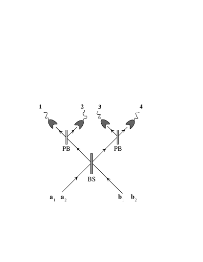
To illustrate the formalism we look at the Innsbruck detection scheme [17] (fig. 1), which consists of 8 POVM elements, corresponding to the events
Only the first four events allow assigning unambiguously Bell states to the outcomes. The total fraction of these events for teleportation, where all Bell states are equally probable, is . The state demolishing projection on entangled states is indeed possible using only linear elements, but not 100 % efficient.
II Description of the considered measurements
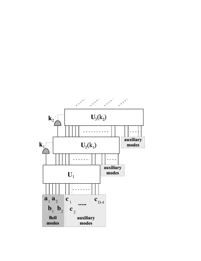
Before we continue we shall describe our tools more precisely. We restrict our measurement apparatus to linear elements only. This means that the vector of creation operators of the input modes is mapped by a unitary matrix onto the vector of creation operators of the output modes. Reck et al. [18] have shown that all these unitary mappings can be realized using only beam splitters and phase shifters. The number of modes is not necessarily four: we can couple to more modes using beam-splitters so that the input states are described by the direct product of the Hilbert space of the Bell states and the initial state of the additional modes. All those modes are mapped into output modes, where place detectors. We assume these detectors to be ideal, so that they are described as performing a POVM measurement on the monitored mode where each POVM element is the projection onto a Fock state of that mode. For experimental reasons, one would like to reduce this to a simpler detector that can not distinguish the number of photons by which it is triggered. The simple “click” or “no click” detector is described by a POVM with two elements, and . However, we will show that even a more fancier detector does not allow us to implement a Bell measurement that never fails. The last tool introduced here is the ability to perform conditional measurements. With that we mean that we monitor one selected mode while keeping the other modes in a waiting loop. Then we can perform some linear operation on the remaining modes depending on the outcome of the measurement with all the tools described above. The general strategy is shown schematically in figure 2.
Vaidman and Yoran [15] have arrived to the conclusion that a Bell state analyzer can not be build using only linear devices, but their measurement apparatus does only a very restrictive type of measurement. It is not allowed to make use of auxiliary photons and no conditional measurements are allowed neither. Both tools might be very useful and we do not see any essential reason to disregard them. For instance the apparatus proposed by Vaidman and Yoran can not distinguish between the four disentangled basis-states of the from,
for which a conditional measurement is needed.
III Criticism to a priori arguments against linear Bell measurements
Intuitively, one needs to operate a “non-linear” measuring device to perform Bell measurements in the sense that one two-level has to interact with the other. In the case of photons there is no direct interaction between them. One can try to couple them through a third system such as an atom [19] or map the state of the photons into atom or ion states and perform there the desired measurement [20]. These schemes are closest to the simple idea of performing a CNOT operation, a Hadamard transform and than projecting on the disentangled base, but they bring up a whole new range of problems (e.g. weak coupling, decoherence, pulse shape design) that breaks with the idea of having simple and controlled “table-top” optical implementations of Quantum Information applications. Therefore it is worth checking the possibility of performing it by linear means.
It is true that linear operations can not make the two input photons interact, they can only make them interfere. Therefore the unitary transformation is separable in the sense that it can be written in terms of a unitary operation over each photon, and of course a CNOT can not be performed by these means ( acts on the symmetric subspace of the single photon Hilbert space product , dim ). Even if this kind of operation preserves the entanglement, the Hilbert space might be large enough to span outputs which trigger different combination of detectors for different input Bell state.
IV No-Go Theorem
We now show that it is not possible to construct a Bell measurement using only the tools mentioned above to realize a measurement, for which all POVM elements are projections on one of the four orthogonal Bell states.
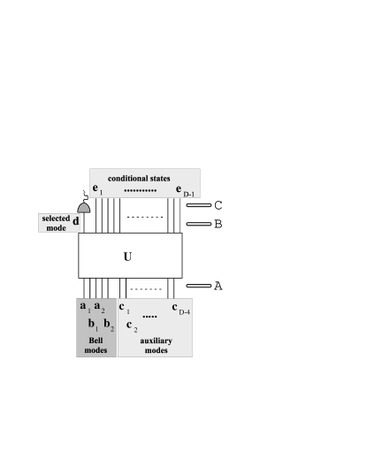
To do so we concentrate on the first step of our measurement set-up: We measure the photon number in one selected mode (see figure 3). For each result we will find the remaining modes in four conditional states corresponding to each Bell state input. We then show that there is always at least one photon number detection event in the first mode that leads to non-orthogonal (i.e. not distinguishable) conditional states in the remaining modes.
In stage A (fig. 3) the input state can be described as a product of two polynomials in the creation operators of the auxiliary and the Bell states modes respectively acting onto the vacuum (denoted by ):
Since we use detectors with photon number resolution it is enough to assume that the auxiliary input is in a state of definite photon number. Then contains only products of a fixed number of creation operators, and contains only products of two creation operators. Now the modes of the Bell state input and the auxiliary modes are linearly mapped by the unitary transformation into the output modes and . At stage B the state is described by
We expand the two polynomials in powers of as
| (5) | |||||
| (6) |
is defined as the maximal order in among the four polynomials and it is independent of the index . As a consequence, the polynomials can be zero for some . Similarly is defined as the order in of the polynomia .
In the mode we will find a range of photon numbers. To prove the theorem it suffices to see that for any of these events the conditional states that arise for each of the Bell states, are not perfectly distinguishable. We concentrate on the measurement outcomes in this mode which leads to the maximum photon number detected in that mode, . The states of the remaining modes conditioned on the occurrence of this event is then given by
| (7) |
The reason of starting out from the event of detecting the photons in the selected mode , is that the problem reduces to a much simpler form in which the measuring apparatus is not allowed to make use of auxiliary photons. That is, by imposing the orthogonality condition of the conditional states on this particular event, we prove that the contribution of the auxiliary photons can not make non-orthogonal states orthogonal in the sense that two conditional states are orthogonal if and only if the the states,
are orthogonal.
To prove this statement we observe that the overlap of two conditional states belonging to different Bell state input and is given by
| (8) | |||||
| (9) | |||||
| (10) |
The first step makes use of the commutativity of and following the commutativity of the two set of creation operators for the auxiliary modes and the Bell modes. Furthermore, the first step inserts the identity operator of the Fock space for all involved modes. We denote by the vector of photon numbers in each involved mode. The second step then uses the fact that only one of these terms is nonzero. This is a consequence of being a state with total photon number while the conjugate state is a two photon state if and only if .
Now that is clear that the use of auxiliary photons does not provide any help in building a Bell state analyzer, it is much easier to check if the orthogonality condition of the conditional states is fulfilled when only one or two photons are detected in the selected mode . To do this, we introduce a formalism for the linear mapping of modes.
Consider the unnormalized input state
| (12) | |||||
By choosing one of the weights as one and the others as zero, we recover the four Bell states. This state can be written with the help of a symmetric real matrix as
with
A linear transformation of the modes is now equivalent to the transformation
for some matrix of dimension (with ) satisfying . The choice corresponds to an enlargement of the number of modes due to additional unexcited input modes of beam-splitters. The output modes are now . The entries of the matrix reveal the distinguishability of the Bell states in the following way: if two photons are detected in the mode then the presence of in the matrix element reveals which Bell states could have contributed to this event. For all Bell states that contribute, the conditional state of the remaining modes is vacuum. It turns out that this event can not be attributed to a single Bell state. To prove this statement we calculate with a general first column of the matrix given as :
| (13) | |||||
| (15) | |||||
To be able to attribute the event of two photons in one mode unambiguously to one Bell state, one and only one of the coefficients of the ’s should be non zero. It is easily verified that this condition can not be satisfied.
If we impose that three of the coefficients vanish we obtain two possible solutions,
| , | (16) | ||||
| , | (17) |
But for both solutions . Therefore a perfect Bell analyzer can never detect two photons in the selected mode. Now we have left only the case where only one photon is detected.
After a single photon detection at mode , the first line of , denoted by tells us the state of the remaining modes. Their state is derived from the unnormalized state
by choosing, as before, one of the to one, and the rest to zero. We have shown above that the first column of is of the form or in order to avoid two photons entering the selected mode. Due to the symmetry of the problem we can restrict ourselves to the first situation, . We now write in the form
Here are dimensional row vectors. Then is given by
| (19) | |||||
From this it follows that the conditional states are (up to normalization)
| (20) | |||||
| (21) | |||||
| (22) | |||||
| (23) |
with the vector of creation operators . The six different overlaps between these states are (up to the missing normalization factors):
| (24) | |||||
| (25) | |||||
| (26) | |||||
| (27) | |||||
| (28) | |||||
| (29) |
These overlaps are zero if,
| (30) | |||||
| (31) | |||||
| (32) | |||||
| (33) |
Since the column vector can not be a zero vector () this simplifies to
| (34) | |||||
| (35) | |||||
| (36) |
from which we can conclude that . But for this choice the matrix does not have rank and so the restriction on given by can no longer be satisfied. Obviously now we can discard the only remaining case; the zero photon case represents a bad choice of the mode since it would be disconnected from the incoming Bell modes. This is the final blow to the attempt to do Bell measurements with linear elements.
V Conclusion
In this paper we have shown that no experimental set-up using only linear elements can implement a Bell state analyzer. Even the “non-linear experimentalist” performing photon number measurements and acting conditioned on the measurement result can not achieve a Bell measurement which never fails. Included in the proof is the possibility to insert entangled states in auxiliary modes into the measurement device.
Recently there has been another proof of this no-go theorem [15] and some proposals to surmount the theorem [10, 13, 14, 17]. In this paper we have discussed their oversights or drawbacks and explained why the theorem does not apply to them.
The remaining open question is the one for the maximal fraction of successful Bell measurements. The Innsbruck scheme gives . It should be noted, that in principle all numbers between and, in a limit, can be allowed by a POVM measurement, which either gives the correct Bell state or gives an inconclusive result. Something that can help to gain some insight on the problem is to investigate the possibility of projecting with (or asymptotically close to) 100% efficiency over a not maximally entangled base (but still with some entanglement).
The fact that the first step in our proof was to rule out the use of an auxiliary system, does not mean that it could not be a very useful tool when considering the case of obtaining an efficiency bigger than 50 %. Following the same procedure than in this proof, and trying to evaluate the maximum distinguishability of the conditional states [21] that appear in each stage, could be a way to obtain the real upper-bound to the Bell measurement efficiency.
VI Acknowledgments
The authors thank the organizers of the ISI (Italy) and Benasque Center for Physics (Spain) workshops on quantum computation and quantum information held in summer 1998 which brought us in contact with the works by Vaidman and Yoran [15], and Kwiat and Weinfurter [13]. We also thank L. Vaidman and M. Plenio for useful discussions and the Academy of Finland for financial support.
REFERENCES
- [1] C. H. Bennett, G. Brassard, C. Crépeau, R. Jozsa, A. Peres, and W. K. Wootters, Phys. Rev. Lett. 70, 1895 (1993).
- [2] C. H. Bennett and S. J. Wiesner, Phys. Rev. Lett. 69, 2881 (1992).
- [3] A. K. Ekert, Phys. Rev. Lett. 67, 661 (1991).
- [4] Jian-Wei Pan, D. Bouwmeester, H. Weinfurter, and A. Zeilinger, Phys. Rev. Lett. 80, 3891 (1998).
- [5] M. Zukowski, A. Zeilinger, M. A. Horne, and A. K. Ekert, Phys. Rev. Lett. 71, 4287 (1993).
- [6] A. Zeilinger, M. A. Horne, H. Weinfurter, and M. Zukowski, Phys. Rev. Lett. 78, 3031 (1997).
- [7] S. Bose, V. Vedral, and P. L. Knight, Phys. Rev. A 57, 822 (1998).
- [8] P. G. Kwiat, K. Mattle, H. Weinfurter, A. Zeilinger, A. V. Sergienko, and Y. H. Shih, Phys. Rev. Lett. 75, 4337 (1995).
- [9] N. J. Cerf, C. Adami, and P. G. Kwiat, Phys. Rev. A 57, R1477 (1998).
- [10] D. Boschi, S. Branca, F. De Martini, L. Hardy, and S. Popescu, Phys. Rev. Lett. 80, 1121 (1998).
- [11] D. Bouwmeester, J. W. Pan, K. Mattle, M. Eibl, H. Weinfurter, and A. Zeilinger, Nature 390, 575 (1997).
- [12] K. Mattle, H. Weinfurter, P. G. Kwiat, and A. Zeilinger, Phys. Rev. Lett. 76, 4656 (1996).
- [13] P. G. Kwiat and H. Weinfurter, to be published.
- [14] S. L. Braunstein and H. J. Kimble, Phys. Rev. Lett. 80, 869 (1998).
- [15] L. Vaidman and N. Yoran, e-print quant-ph/9808043.
- [16] A. Peres, Quantum Theory, Concepts and Methods (Kluwer, Dordrecht, 1993); C. W. Helstrom Quantum Detection and Estimation Theory (Academic Press, New York, 1976)
- [17] H. Weinfurter, Europhys. Lett. 25, 559 (1994); S. L. Braunstein and A. Mann, Phys. Rev. A 51, R1727 (1995); M. Michler, K. Mattle, H. Weinfurter, and A. Zeilinger, Phys. Rev. A 53, R1209 (1996).
- [18] M. Reck, A. Zeilinger, H. J. Bernstein, and P. Bertani, Phys. Rev. Lett. 73, 58 (1994).
- [19] P. T rm and S. Stenholm, Phys. Rev. A 54, 4701 (1996)
- [20] S. J. van Enk, J. I. Cirac, P. Zoller, Phys. Rev. Lett. 79, 5178 (1997)
- [21] A. Chefles and S. M. Barnett, e-print quant-ph/9807023; A. Peres and D. R. Terno, e-print quant-ph/9804031; A. Chefles, Phys. Lett. A 239, 339 (1998).