Quantile Motion and Tunneling

Abstract

The concepts of quantile position, trajectory, and velocity are defined. For a tunneling quantum mechanical wave packet, it is proved that its quantile position always stays behind that of a free wave packet with the same initial parameters. In quantum mechanics the quantile trajectories are mathematically identical to Bohm’s trajectories. A generalization to three dimensions is given.

, , and

The discussion of tunneling times has a long history in the literature, for a review see [1]. Recent developments are, e.g., the “tunneled flux” approach [2], the operational projector approach to tunneling times [3], and the calculation of tunneling times in the framework of the Dirac equation [4]. Among other findings it has been reported that the velocity of a particle can be larger within a repulsive barrier than outside the barrier and that instantaneous tunneling can occur. Great care has to be exercised, however, in defining a velocity in quantum mechanics, since the velocity definition of classical mechanics requires the concept of a trajectory for a point particle which breaks down in quantum mechanics. In this letter we introduce a definition of a velocity which is strictly based on probability concepts.

1 Definitions

For any probability density $\varrho(x)$ the quantile $x_{Q}$ associated with the probability $Q$ is defined in the mathematical literature, c.f., e.g., [5, 6], by

$$Q=\int_{-\infty}^{x_{Q}}\varrho(x)\,{\rm d}x\>.$$

For a position- and time-dependent probability density $\varrho(x,t)$ we introduce the time-dependent quantile position $x_{P}(t)$ through

$$P=\int_{x_{P}(t)}^{\infty}\varrho(x,t)\,{\rm d}x\>.$$ (1)

The change to the complementary integration interval is chosen merely for convenience. Essential is the transfer of the quantile concept from a probability density in mathematical statistics to a space- and time-dependent distribution describing a physics problem. It yields for every time $t$ a well-defined point $x_{P}(t)$. Considering $x=x_{P}(t)$ as a quantile trajectory we define the quantile velocity $v_{P}(t)={\rm d}x_{P}/{\rm d}t$, which obviously depends on the chosen value of $P$.

In the case of a conserved probability the corresponding probability density fulfills the continuity equation of the form

$$\frac{\partial\varrho}{\partial t}(x,t)+\frac{\partial j}{\partial x}(x,t)=0\>,$$ (2)

$j(x,t)$ being the corresponding probability current density vanishing at infinity. Equations (1) and (2) permit a direct calculation of the quantile velocity $v_{P}(t)$. Differentiating (1) with respect to time we immediately obtain

$$v_{P}=\frac{{\rm d}x_{P}}{{\rm d}t}=\frac{j(x_{P},t)}{\varrho(x_{P},t)}\>.$$ (3)

Equation (3) is an ordinary differential equation for the quantile position $x_{P}(t)$, an implicit solution of which is given by (1).

In an experiment with quantum-mechanical wave packets the quantile velocity can be determined on a statistical basis by time-of-flight measurements: One prepares by the same procedure $N$ single-particle wave packets and sets a clock to zero at the moment at which the spatial expectation value of a wave packet leaves the source. With a detector placed at position $x_{1}$ one registers the arrival times $t_{1m}$ of particles for $m=1,2,\dots,N$ and orders them such that $t_{11}<t_{12}<\ldots$. One picks the time $t_{1n}$ which is the largest of the smallest $n$ times and chooses $n/N=P$. The time $t_{1n}$ is the arrival time of the quantile $x_{P}$ at the position $x_{1}$, i.e., $x_{P}(t_{1n})=x_{1}$. By repeating the experiment with a detector at $x_{2}$ one obtains $t_{2n}$, etc. The points $x_{P}(t_{in})$ are discrete points on the quantile trajectory $x=x_{P}(t)$. If $x_{1}$ and $x_{2}$ mark the beginning and the end of a potential barrier then $t_{2n}-t_{1n}$ is the quantile traversal time of the barrier.

In the case of classical systems, e.g., classical electrodynamics, the quantile velocity can quite naturally be interpreted as velocity of an electromagnetic signal. We identify the density $\varrho(x,t)=w(x,t)/W$ with the ratio of the electromagnetic energy density $w$ and the total energy $W$ of the pulse. We say the signal has left the transmitter, if the fraction $P$ of the total energy has left the transmitter. It has reached the detector if the fraction $P$ has been absorbed by the detector. Obviously a minimum amount of energy (the threshold energy $W_{\rm th}$) is needed in the detector to register a signal. One will therefore choose $P$ such that $PW\geq W_{\rm th}$.

2 Free wave packet

As an example we consider the time development of a time-dependent Gaussian probability distribution

$$\varrho(x,t)=\frac{1}{\sqrt{2\pi}\sigma_{x}(t)}\exp\left\{-\frac{(x-\bar{x}-\bar{v}t)^{2}}{2\sigma_{x}^{2}(t)}\right\}\,,\;\;\sigma^{2}_{x}(t)=\sigma^{2}_{x0}\left(1+\frac{\sigma^{2}_{v}t^{2}}{\sigma^{2}_{x0}}\right)\,.$$ (4)

This probability density describes just as well (i) the marginal distribution of a bivariate Gaussian phase-space distribution of a classical assembly (see, e.g., [7]) of force-free particles of mass $m$ with initial position expectation value $\bar{x}$, initial spatial variation $\sigma_{x0}$, and momentum expectation value $\bar{p}=m\bar{v}$, momentum variation $\sigma_{p}=\hbar/(2\sigma_{x0})$, and velocity variation $\sigma_{v}=\sigma_{p}/m$, and (ii) the spatial probability distribution of a quantum-mechanical force-free Gaussian wave packet with the same initial parameters as the above classical distribution. Equation (1) yields the quantile trajectories

$$x_{P}(t)=\bar{x}+\bar{v}t+(\sigma_{x}(t)/\sigma_{x0})(x_{0}-\bar{x})\>,\quad$$

and thus the quantile velocities

$$v_{P}(t)=\bar{v}+\left(\sigma_{v}^{2}\,t/(\sigma_{x}(t)\sigma_{x0})\right)(x_{0}-\bar{x})\>.$$

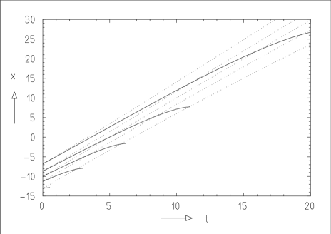
Figure 1: Quantile trajectories for the wave packet (4) (dotted lines) and (5) (solid lines). Trajectories are plotted for values of $P$ between $0.1$ and $0.9$ in steps of $\Delta P=0.2$. In all figures positions are given in units $\hbar/\sqrt{{\rm eV}m}$ and times in units $\hbar/{\rm eV}$ with $m$ being the mass of the particle. At time $t=0$ the wave packet is in both cases a Gaussian wave packet with mean position $\bar{x}=-10\hbar/\sqrt{{\rm eV}m}$, mean momentum $\bar{p}=2\sqrt{{\rm eV}m}$, and momentum width $\sigma_{p}=0.2\sqrt{{\rm eV}m}$. The wave packet (5) is additionally characterized by a probability loss of temporal rate $\lambda=0.1\hbar/{\rm eV}$.

Here $x_{0}=x_{P}(0)$ is the initial quantile position associated with $P$ according to the condition $(1/2)\mathop{\rm erfc}[(x_{0}-\bar{x})/(\sqrt{2}\sigma_{x0})]=P$. If we take (4) to be a classical phase-space distribution, we note that the quantile trajectories $x=x_{P}(t)$ are not trajectories of free particles possessing constant velocities $v=p/m$. Only for $P=\frac{1}{2}$, i.e., $x_{0}=\bar{x}$ is the quantile trajectory identical to a particle trajectory. Quantile trajectories of a free wave packet for different values of $P$ are shown as dotted lines in Fig. 1.

3 Quantile motion for a non-conserved probability

Our definition (1) allows a consistent description of motion also in the case of a non-conserved probability. We assume that instead of a normalization to one at all times, we have a loss of probability,

$$\int_{-\infty}^{\infty}\varrho(x,t)\,{\rm d}x=F(t)\leq 1\>,\quad F(0)=1\>.$$

As an illustration we consider again the time development of a wave packet prepared at $t=0$ to be a Gaussian distribution with the same parameters as in (4). In addition we introduce a temporal exponential decrease of the probability to find the particle anywhere in space, as for example caused by the presence of a constant purely imaginary potential. Thus the probability density may be written in the form

$$\varrho_{\lambda}(x,t)=\frac{1}{\sqrt{2\pi}\sigma_{x}(t)}\exp\left\{-\frac{(x-\bar{x}-\bar{v}t)^{2}}{2\sigma_{x}^{2}(t)}\right\}\exp\left\{-\lambda t\right\}\>,$$ (5)

where $\lambda$ is the temporal rate of probability loss and $\sigma_{x}(t)$ is given in equation (4). Instead of the continuity equation (2) we have now

$$\frac{\partial\varrho_{\lambda}}{\partial t}(x,t)+\frac{\partial j_{\lambda}}{\partial x}(x,t)=-l(x,t)\>,$$ (6)

$j_{\lambda}(x,t)$ being the current density of the non-conserved probability and $l(x,t)=\lambda\varrho_{\lambda}(x,t)\geq 0$ describing the density of the temporal loss rate. For the quantile position $x_{P}(t)$ we obtain the integro-differential equation

$$\frac{{\rm d}x_{P}(t)}{{\rm d}t}=\frac{j_{\lambda}(x_{P},t)}{\varrho_{\lambda}(x_{P},t)}-\frac{1}{\varrho_{\lambda}(x_{P},t)}\int_{x_{P}(t)}^{\infty}l(x^{\prime},t)\,{\rm d}x^{\prime}\>.$$ (7)

The solid lines in Fig. 1 are quantile trajectories for different values of $P$. The curves end at the quantile position $x_{P\rm max}$ where the integral over the loss rate on the right–hand side of (7) equals the probability current density $j_{\lambda}(x,t)$. At later times the probability loss term in (7) dominates over the probability current density $j_{\lambda}(x,t)$. For positions at values $x>x_{P\rm max}$ the condition (1) can no longer be satisfied. Note that the formulation of quantile motion for a non-conserved probability has general validity, since Eqs. (6) and (7) do not depend on the details of the probability loss.

4 Tunneling

In the following we show that for the same value of $P$ and for two identically prepared, tunneling and free wave packets, the quantile position of the tunneling wave packet in the transmission region of the potential remains at any given time $t$ behind the quantile position of the free wave packet, i.e., the arrival time of the tunneled quantile behind the barrier is always later than that of the free wave packet. We consider the tunneling of a wave packet with spectral function $\widetilde{\psi}(k)$ in momentum space through a repulsive square potential barrier, $V(x)=V\geq 0$ for $|x|<a$ and $V(x)=0$ for $|x|>a$. The probability densities of the tunneling and of the free wave packet with the same spectral function $\widetilde{\psi}(k)$ are denoted by $\varrho_{\rm T}(x,t)$ and $\varrho_{\rm F}(x,t)$, respectively. The functions

$$P_{\rm T}(x,t)=\int_{x}^{\infty}\varrho_{\rm T}(x^{\prime},t)\,{\rm d}x^{\prime}\>,\qquad P_{\rm F}(x,t)=\int_{x}^{\infty}\varrho_{\rm F}(x^{\prime},t)\,{\rm d}x^{\prime}$$

give the probabilities at time $t$ for the tunneling and the free particle to be found to the right of the position $x$ in the transmission region $x>a$ of the potential. Since $P_{\rm T}(x,t)$ and $P_{\rm F}(x,t)$ decrease monotonically with $x$, our statement is always true if the condition

$$\Delta P(x,t)=P_{\rm F}(x,t)-P_{\rm T}(x,t)\geq 0$$ (8)

for $x>a$ is fulfilled. We consider a wave packet described by a spectral function $\widetilde{\psi}(k)$ with a positive wave number spectrum, i.e., $\widetilde{\psi}(k)=0$ for $k<0$. The difference $\Delta P(x,t)$ in the region $x>a$ is

$$\Delta P(x,t)=\frac{{\rm i}}{2\pi}\int_{0}^{\infty}\int_{0}^{\infty}[1-T(k^{\prime})T^{*}(k^{\prime\prime})]\frac{\widetilde{\psi}(k^{\prime};x,t)\widetilde{\psi}^{*}(k^{\prime\prime};x,t)}{k^{\prime}-k^{\prime\prime}+{\rm i}\varepsilon}\,{\rm d}k^{\prime}{\rm d}k^{\prime\prime}\>,$$

where $\widetilde{\psi}(k;x,t)=\widetilde{\psi}(k)\exp[{\rm i}k(x-\bar{x})-{\rm i}\hbar k^{2}t/(2m)]$ and

$$T(k)=\frac{4k\gamma}{{\cal D}(k)}\>,\qquad{\cal D}(k)=(k+\gamma)^{2}{\rm\/e\/}^{2{\rm i}a(k-\gamma)}-(k-\gamma)^{2}{\rm\/e\/}^{2{\rm i}a(k+\gamma)}\>,$$

is the transmission amplitude in momentum space for the repulsive square potential barrier ($\gamma=(k^{2}-2mV/\hbar^{2})^{1/2}$). We consider $\Delta P(x,t)$ as the limiting function of a series of parameterized functions

$$\begin{array}[]{rcl}\Delta P_{\lambda}(x,t)&=&\displaystyle\frac{{\rm i}}{2\pi}\int_{0}^{\infty}\int_{0}^{\infty}\frac{{\cal D}_{\lambda}(k^{\prime}){\cal D}_{\lambda}^{*}(k^{\prime\prime})-16k^{\prime}k^{\prime\prime}\gamma^{\prime}\gamma^{\prime\prime*}}{{\cal D}(k^{\prime}){\cal D}^{*}(k^{\prime\prime})}\\[15.0pt] &\times&\displaystyle\frac{\widetilde{\psi}(k^{\prime};x,t)\widetilde{\psi}^{*}(k^{\prime\prime};x,t)}{k^{\prime}-k^{\prime\prime}+{\rm i}\varepsilon}\,{\rm d}k^{\prime}{\rm d}k^{\prime\prime}\end{array}$$

for $\lambda\to 1$, where ${\cal D}_{\lambda}(k)=(k+\gamma)^{2}{\rm\/e\/}^{2{\rm i}a\lambda(k-\gamma)}-(k-\gamma)^{2}{\rm\/e\/}^{2{\rm i}a\lambda(k+\gamma)}$. Thus, we have $\Delta P_{\lambda}(x,t)=0$ for $\lambda=0$, so that the difference of probabilities is

$$\Delta P(x,t)=\int_{0}^{\scriptscriptstyle 1}\frac{\partial{}}{\partial{}\lambda}\Delta P_{\lambda}(x,t)\,{\rm d}\lambda\>.$$ (9)

Explicitly calculating the derivative in (9) yields

$$\begin{array}[]{rcl}\Delta P(x,t)&=&\displaystyle\frac{2a}{\pi}\left(\frac{4mV}{\hbar^{2}}\right)\left\{\int_{0}^{\scriptscriptstyle 1}\left|\,\int_{0}^{\infty}\frac{{\cal Z}_{\lambda}(k)}{{\cal D}(k)}\widetilde{\psi}(k;x,t)\,{\rm d}k\,\right|^{2}{\rm d}\lambda\right.\\[17.0pt] &+&\displaystyle 4\left(\frac{4mV}{\hbar^{2}}\right)\int_{0}^{\scriptscriptstyle 1}\left|\,\int_{0}^{\infty}\frac{{\rm\/e\/}^{2{\rm i}a\lambda k}\sin(2a\lambda\gamma)}{{\cal D}(k)}\widetilde{\psi}(k;x,t)\,{\rm d}k\,\right|^{2}{\rm d}\lambda\\[17.0pt] &+&\displaystyle\left.\left(\frac{4mV}{a\hbar^{2}}\right)\int_{x}^{\infty}\left|\,\int_{0}^{\infty}\frac{{\rm\/e\/}^{2{\rm i}ak}\sin(2a\gamma)}{{\cal D}(k)}\widetilde{\psi}(k;x^{\prime},t)\,{\rm d}k\,\right|^{2}{\rm d}x^{\prime}\right\}\>,\end{array}$$ (10)

where ${\cal Z}_{\lambda}(k)=(k+\gamma){\rm\/e\/}^{2{\rm i}a\lambda(k-\gamma)}-(k-\gamma){\rm\/e\/}^{2{\rm i}a\lambda(k+\gamma)}$. The positivity of (10) proves the condition (8) and therefore the initial statement on the retardation of the quantile trajectory of the tunneled wave packet in the transmission region of the potential. This procedure can be extended to the case of a general non-negative potential $V(x)$ of finite range, introducing a segmentation of the potential into thin square potential barriers and then similarly parameterizing the difference $\Delta P(x,t)$ to obtain a positive-definite expression [8].

In Fig. 2a the time development of a wave packet incident on a barrier is shown. The packet is partly reflected and partly transmitted. In Fig. 2b the quantile trajectories $x=x_{P}(t)$ for the same problem are presented. For small values of $P$ the trajectories penetrate the barrier, for larger values they reverse their direction. We observe that in all cases the quantile velocity within the barrier region is smaller in absolute value than far from the barrier.

5 Relation to Bohmian mechanics

Bohm’s interpretation of quantum mechanics [9] introduces particle trajectories $x=x(t)$ satisfying the equation of motion ${\rm d}x(t)/{\rm d}t=j(x(t),t)/\varrho(x(t),t)$. For the solution of this differential equation the initial condition $x(0)=x_{0}$ is needed as a hidden parameter. If we set Bohm’s initial position $x_{0}$ equal to the initial quantile position $x_{P}(0)$ the quantile trajectories are mathematically identical to Bohm’s particle trajectories. Conceptually, however, they are based on the probability interpretation of the conventional quantum mechanics.

Leavens and Aers [10] and Spiller et al. [11] realized that Bohm’s interpretation of quantum mechanics — reintroducing the point-particle concept — offers the opportunity of unambiguously defining the velocity as in classical mechanics (see also [12, 13]). In contrast to their work our approach is based on the conventional probabilistic concepts and does not depend on the interpretation given by Bohm. In Ref. [10] tunneling times are given which are based on the concept of Bohm trajectories. McKinnon and Leavens [14] pointed out the significance with respect to tunnel times of a particular Bohm trajectory for $P=|T|^{2}$, with $|T|^{2}$ being the transmission probability. Wu and Sprung [15] have discussed quantum probability patterns for stationary problems.

6 Generalization to three dimensions

The equivalence of equations (1) and (3) has been noticed before, see, e.g., [12, 16]. In [12] it was considered as an artifact of low dimensionality. In both papers, this equivalence was not related to the probability interpretation made possible by equation (1). However, the generalization to three dimensions is straightforward, if one considers that the interval between two quantile positions $x_{P_{1}}(t)$ and $x_{P_{2}}(t)$ always contains the same amount of probability $Q=P_{1}-P_{2}$ and that all trajectories with initial positions $x_{P_{1}}(0)<x_{P}(0)<x_{P_{2}}(0)$ stay in the interval $x_{P_{1}}(t)<x_{P}(t)<x_{P_{2}}(t)$. This suggests that in three dimensions trajectories defined by the equation of motion

$$\frac{\partial\mathchoice{\mbox{\boldmath$\displaystyle\bf x$}}{\mbox{\boldmath$\textstyle\bf x$}}{\mbox{\boldmath$\scriptstyle\bf x$}}{\mbox{\boldmath$\scriptscriptstyle\bf x$}}_{P}(t,\mathchoice{\mbox{\boldmath$\displaystyle\bf x$}}{\mbox{\boldmath$\textstyle\bf x$}}{\mbox{\boldmath$\scriptstyle\bf x$}}{\mbox{\boldmath$\scriptscriptstyle\bf x$}})}{\partial t}=\mathchoice{\mbox{\boldmath$\displaystyle\bf v$}}{\mbox{\boldmath$\textstyle\bf v$}}{\mbox{\boldmath$\scriptstyle\bf v$}}{\mbox{\boldmath$\scriptscriptstyle\bf v$}}(\mathchoice{\mbox{\boldmath$\displaystyle\bf x$}}{\mbox{\boldmath$\textstyle\bf x$}}{\mbox{\boldmath$\scriptstyle\bf x$}}{\mbox{\boldmath$\scriptscriptstyle\bf x$}}_{P},t)=\frac{\mathchoice{\mbox{\boldmath$\displaystyle\bf j$}}{\mbox{\boldmath$\textstyle\bf j$}}{\mbox{\boldmath$\scriptstyle\bf j$}}{\mbox{\boldmath$\scriptscriptstyle\bf j$}}(\mathchoice{\mbox{\boldmath$\displaystyle\bf x$}}{\mbox{\boldmath$\textstyle\bf x$}}{\mbox{\boldmath$\scriptstyle\bf x$}}{\mbox{\boldmath$\scriptscriptstyle\bf x$}}_{P},t)}{\varrho(\mathchoice{\mbox{\boldmath$\displaystyle\bf x$}}{\mbox{\boldmath$\textstyle\bf x$}}{\mbox{\boldmath$\scriptstyle\bf x$}}{\mbox{\boldmath$\scriptscriptstyle\bf x$}}_{P},t)}$$ (11)

and having initial positions $\mathchoice{\mbox{\boldmath$\displaystyle\bf x$}}{\mbox{\boldmath$\textstyle\bf x$}}{\mbox{\boldmath$\scriptstyle\bf x$}}{\mbox{\boldmath$\scriptscriptstyle\bf x$}}_{P}(0,\mathchoice{\mbox{\boldmath$\displaystyle\bf x$}}{\mbox{\boldmath$\textstyle\bf x$}}{\mbox{\boldmath$\scriptstyle\bf x$}}{\mbox{\boldmath$\scriptscriptstyle\bf x$}})=\mathchoice{\mbox{\boldmath$\displaystyle\bf x$}}{\mbox{\boldmath$\textstyle\bf x$}}{\mbox{\boldmath$\scriptstyle\bf x$}}{\mbox{\boldmath$\scriptscriptstyle\bf x$}}$ within a volume $V$ containing an amount $P$ of probability stay within a volume $V_{t}$ containing the same amount of probability. To prove this statement we introduce the time-dependent base of tangent vectors $\mathchoice{\mbox{\boldmath$\displaystyle\bf\eta$}}{\mbox{\boldmath$\textstyle\bf\eta$}}{\mbox{\boldmath$\scriptstyle\bf\eta$}}{\mbox{\boldmath$\scriptscriptstyle\bf\eta$}}{}^{i}(t,\mathchoice{\mbox{\boldmath$\displaystyle\bf x$}}{\mbox{\boldmath$\textstyle\bf x$}}{\mbox{\boldmath$\scriptstyle\bf x$}}{\mbox{\boldmath$\scriptscriptstyle\bf x$}})=\partial\mathchoice{\mbox{\boldmath$\displaystyle\bf x$}}{\mbox{\boldmath$\textstyle\bf x$}}{\mbox{\boldmath$\scriptstyle\bf x$}}{\mbox{\boldmath$\scriptscriptstyle\bf x$}}_{P}(t,\mathchoice{\mbox{\boldmath$\displaystyle\bf x$}}{\mbox{\boldmath$\textstyle\bf x$}}{\mbox{\boldmath$\scriptstyle\bf x$}}{\mbox{\boldmath$\scriptscriptstyle\bf x$}})/\partial x_{i}$, where $i=1,2,3$. Their Jacobian is given by the expression $D(t,\mathchoice{\mbox{\boldmath$\displaystyle\bf x$}}{\mbox{\boldmath$\textstyle\bf x$}}{\mbox{\boldmath$\scriptstyle\bf x$}}{\mbox{\boldmath$\scriptscriptstyle\bf x$}})=\mathchoice{\mbox{\boldmath$\displaystyle\bf\eta$}}{\mbox{\boldmath$\textstyle\bf\eta$}}{\mbox{\boldmath$\scriptstyle\bf\eta$}}{\mbox{\boldmath$\scriptscriptstyle\bf\eta$}}{}^{1}(t,\mathchoice{\mbox{\boldmath$\displaystyle\bf x$}}{\mbox{\boldmath$\textstyle\bf x$}}{\mbox{\boldmath$\scriptstyle\bf x$}}{\mbox{\boldmath$\scriptscriptstyle\bf x$}})\cdot[\mathchoice{\mbox{\boldmath$\displaystyle\bf\eta$}}{\mbox{\boldmath$\textstyle\bf\eta$}}{\mbox{\boldmath$\scriptstyle\bf\eta$}}{\mbox{\boldmath$\scriptscriptstyle\bf\eta$}}{}^{2}(t,\mathchoice{\mbox{\boldmath$\displaystyle\bf x$}}{\mbox{\boldmath$\textstyle\bf x$}}{\mbox{\boldmath$\scriptstyle\bf x$}}{\mbox{\boldmath$\scriptscriptstyle\bf x$}})\times\mathchoice{\mbox{\boldmath$\displaystyle\bf\eta$}}{\mbox{\boldmath$\textstyle\bf\eta$}}{\mbox{\boldmath$\scriptstyle\bf\eta$}}{\mbox{\boldmath$\scriptscriptstyle\bf\eta$}}{}^{3}(t,\mathchoice{\mbox{\boldmath$\displaystyle\bf x$}}{\mbox{\boldmath$\textstyle\bf x$}}{\mbox{\boldmath$\scriptstyle\bf x$}}{\mbox{\boldmath$\scriptscriptstyle\bf x$}})]$, whereas its time derivative satisfies

$$\frac{\partial D}{\partial t}(t,\mathchoice{\mbox{\boldmath$\displaystyle\bf x$}}{\mbox{\boldmath$\textstyle\bf x$}}{\mbox{\boldmath$\scriptstyle\bf x$}}{\mbox{\boldmath$\scriptscriptstyle\bf x$}})=D(t,\mathchoice{\mbox{\boldmath$\displaystyle\bf x$}}{\mbox{\boldmath$\textstyle\bf x$}}{\mbox{\boldmath$\scriptstyle\bf x$}}{\mbox{\boldmath$\scriptscriptstyle\bf x$}})\mathchoice{\mbox{\boldmath$\displaystyle\bf\nabla$}}{\mbox{\boldmath$\textstyle\bf\nabla$}}{\mbox{\boldmath$\scriptstyle\bf\nabla$}}{\mbox{\boldmath$\scriptscriptstyle\bf\nabla$}}_{\mathchoice{\mbox{\boldmath$\displaystyle\bf x$}}{\mbox{\boldmath$\textstyle\bf x$}}{\mbox{\boldmath$\scriptstyle\bf x$}}{\mbox{\boldmath$\scriptscriptstyle\bf x$}}_{P}}\cdot\mathchoice{\mbox{\boldmath$\displaystyle\bf v$}}{\mbox{\boldmath$\textstyle\bf v$}}{\mbox{\boldmath$\scriptstyle\bf v$}}{\mbox{\boldmath$\scriptscriptstyle\bf v$}}(\mathchoice{\mbox{\boldmath$\displaystyle\bf x$}}{\mbox{\boldmath$\textstyle\bf x$}}{\mbox{\boldmath$\scriptstyle\bf x$}}{\mbox{\boldmath$\scriptscriptstyle\bf x$}}_{P}(t,\mathchoice{\mbox{\boldmath$\displaystyle\bf x$}}{\mbox{\boldmath$\textstyle\bf x$}}{\mbox{\boldmath$\scriptstyle\bf x$}}{\mbox{\boldmath$\scriptscriptstyle\bf x$}}),t)\>.$$

In particular at the initial time $t=0$ we have $D(0)=1$. The total time derivative of the density is then given by

$$\frac{{\rm d}\varrho(\mathchoice{\mbox{\boldmath$\displaystyle\bf x$}}{\mbox{\boldmath$\textstyle\bf x$}}{\mbox{\boldmath$\scriptstyle\bf x$}}{\mbox{\boldmath$\scriptscriptstyle\bf x$}}_{P},t)}{{\rm d}t}=-\varrho(\mathchoice{\mbox{\boldmath$\displaystyle\bf x$}}{\mbox{\boldmath$\textstyle\bf x$}}{\mbox{\boldmath$\scriptstyle\bf x$}}{\mbox{\boldmath$\scriptscriptstyle\bf x$}}_{P},t)\mathchoice{\mbox{\boldmath$\displaystyle\bf\nabla$}}{\mbox{\boldmath$\textstyle\bf\nabla$}}{\mbox{\boldmath$\scriptstyle\bf\nabla$}}{\mbox{\boldmath$\scriptscriptstyle\bf\nabla$}}_{\mathchoice{\mbox{\boldmath$\displaystyle\bf x$}}{\mbox{\boldmath$\textstyle\bf x$}}{\mbox{\boldmath$\scriptstyle\bf x$}}{\mbox{\boldmath$\scriptscriptstyle\bf x$}}_{P}}\cdot\mathchoice{\mbox{\boldmath$\displaystyle\bf v$}}{\mbox{\boldmath$\textstyle\bf v$}}{\mbox{\boldmath$\scriptstyle\bf v$}}{\mbox{\boldmath$\scriptscriptstyle\bf v$}}(\mathchoice{\mbox{\boldmath$\displaystyle\bf x$}}{\mbox{\boldmath$\textstyle\bf x$}}{\mbox{\boldmath$\scriptstyle\bf x$}}{\mbox{\boldmath$\scriptscriptstyle\bf x$}}_{P},t)\>,$$

so that we find the product $p(t,\mathchoice{\mbox{\boldmath$\displaystyle\bf x$}}{\mbox{\boldmath$\textstyle\bf x$}}{\mbox{\boldmath$\scriptstyle\bf x$}}{\mbox{\boldmath$\scriptscriptstyle\bf x$}})=\varrho(\mathchoice{\mbox{\boldmath$\displaystyle\bf x$}}{\mbox{\boldmath$\textstyle\bf x$}}{\mbox{\boldmath$\scriptstyle\bf x$}}{\mbox{\boldmath$\scriptscriptstyle\bf x$}}_{P}(t,\mathchoice{\mbox{\boldmath$\displaystyle\bf x$}}{\mbox{\boldmath$\textstyle\bf x$}}{\mbox{\boldmath$\scriptstyle\bf x$}}{\mbox{\boldmath$\scriptscriptstyle\bf x$}}),t)D(t,\mathchoice{\mbox{\boldmath$\displaystyle\bf x$}}{\mbox{\boldmath$\textstyle\bf x$}}{\mbox{\boldmath$\scriptstyle\bf x$}}{\mbox{\boldmath$\scriptscriptstyle\bf x$}})$ to be time independent,

$$\frac{\partial p}{\partial t}(t,\mathchoice{\mbox{\boldmath$\displaystyle\bf x$}}{\mbox{\boldmath$\textstyle\bf x$}}{\mbox{\boldmath$\scriptstyle\bf x$}}{\mbox{\boldmath$\scriptscriptstyle\bf x$}})=0\>.$$

This implies that an integral over a finite volume $V_{0}$,

$$\int_{V_{0}}p(t,\mathchoice{\mbox{\boldmath$\displaystyle\bf x$}}{\mbox{\boldmath$\textstyle\bf x$}}{\mbox{\boldmath$\scriptstyle\bf x$}}{\mbox{\boldmath$\scriptscriptstyle\bf x$}}{}^{\prime})\,{\rm d}^{3}\mathchoice{\mbox{\boldmath$\displaystyle\bf x$}}{\mbox{\boldmath$\textstyle\bf x$}}{\mbox{\boldmath$\scriptstyle\bf x$}}{\mbox{\boldmath$\scriptscriptstyle\bf x$}}{}^{\prime}=P\>,$$

is time independent. An amount of probability

$$P=\int_{V_{0}}p(0,\mathchoice{\mbox{\boldmath$\displaystyle\bf x$}}{\mbox{\boldmath$\textstyle\bf x$}}{\mbox{\boldmath$\scriptstyle\bf x$}}{\mbox{\boldmath$\scriptscriptstyle\bf x$}}{}^{\prime})\,{\rm d}^{3}\mathchoice{\mbox{\boldmath$\displaystyle\bf x$}}{\mbox{\boldmath$\textstyle\bf x$}}{\mbox{\boldmath$\scriptstyle\bf x$}}{\mbox{\boldmath$\scriptscriptstyle\bf x$}}{}^{\prime}=\int_{V_{0}}\varrho(\mathchoice{\mbox{\boldmath$\displaystyle\bf x$}}{\mbox{\boldmath$\textstyle\bf x$}}{\mbox{\boldmath$\scriptstyle\bf x$}}{\mbox{\boldmath$\scriptscriptstyle\bf x$}},0)\,{\rm d}^{3}\mathchoice{\mbox{\boldmath$\displaystyle\bf x$}}{\mbox{\boldmath$\textstyle\bf x$}}{\mbox{\boldmath$\scriptstyle\bf x$}}{\mbox{\boldmath$\scriptscriptstyle\bf x$}}$$

contained initially in a volume $V_{0}$ is at time $t$ given by

$$P=\int_{V_{0}}\varrho(\mathchoice{\mbox{\boldmath$\displaystyle\bf x$}}{\mbox{\boldmath$\textstyle\bf x$}}{\mbox{\boldmath$\scriptstyle\bf x$}}{\mbox{\boldmath$\scriptscriptstyle\bf x$}}_{P}(t,\mathchoice{\mbox{\boldmath$\displaystyle\bf x$}}{\mbox{\boldmath$\textstyle\bf x$}}{\mbox{\boldmath$\scriptstyle\bf x$}}{\mbox{\boldmath$\scriptscriptstyle\bf x$}}{}^{\prime}),t)D(t,\mathchoice{\mbox{\boldmath$\displaystyle\bf x$}}{\mbox{\boldmath$\textstyle\bf x$}}{\mbox{\boldmath$\scriptstyle\bf x$}}{\mbox{\boldmath$\scriptscriptstyle\bf x$}}{}^{\prime})\,{\rm d}^{3}\mathchoice{\mbox{\boldmath$\displaystyle\bf x$}}{\mbox{\boldmath$\textstyle\bf x$}}{\mbox{\boldmath$\scriptstyle\bf x$}}{\mbox{\boldmath$\scriptscriptstyle\bf x$}}{}^{\prime}\>.$$

The time-dependent substitution $\mathchoice{\mbox{\boldmath$\displaystyle\bf x$}}{\mbox{\boldmath$\textstyle\bf x$}}{\mbox{\boldmath$\scriptstyle\bf x$}}{\mbox{\boldmath$\scriptscriptstyle\bf x$}}=\mathchoice{\mbox{\boldmath$\displaystyle\bf x$}}{\mbox{\boldmath$\textstyle\bf x$}}{\mbox{\boldmath$\scriptstyle\bf x$}}{\mbox{\boldmath$\scriptscriptstyle\bf x$}}_{P}(t,\mathchoice{\mbox{\boldmath$\displaystyle\bf x$}}{\mbox{\boldmath$\textstyle\bf x$}}{\mbox{\boldmath$\scriptstyle\bf x$}}{\mbox{\boldmath$\scriptscriptstyle\bf x$}}{}^{\prime})$ yields

$$P=\int_{V_{t}}\varrho(\mathchoice{\mbox{\boldmath$\displaystyle\bf x$}}{\mbox{\boldmath$\textstyle\bf x$}}{\mbox{\boldmath$\scriptstyle\bf x$}}{\mbox{\boldmath$\scriptscriptstyle\bf x$}},t)\,{\rm d}^{3}\mathchoice{\mbox{\boldmath$\displaystyle\bf x$}}{\mbox{\boldmath$\textstyle\bf x$}}{\mbox{\boldmath$\scriptstyle\bf x$}}{\mbox{\boldmath$\scriptscriptstyle\bf x$}}$$

with the volume $V_{t}$ given by all the points $\mathchoice{\mbox{\boldmath$\displaystyle\bf x$}}{\mbox{\boldmath$\textstyle\bf x$}}{\mbox{\boldmath$\scriptstyle\bf x$}}{\mbox{\boldmath$\scriptscriptstyle\bf x$}}_{P}(t,\mathchoice{\mbox{\boldmath$\displaystyle\bf x$}}{\mbox{\boldmath$\textstyle\bf x$}}{\mbox{\boldmath$\scriptstyle\bf x$}}{\mbox{\boldmath$\scriptscriptstyle\bf x$}})$ at time $t$ lying on trajectories with initial positions $\mathchoice{\mbox{\boldmath$\displaystyle\bf x$}}{\mbox{\boldmath$\textstyle\bf x$}}{\mbox{\boldmath$\scriptstyle\bf x$}}{\mbox{\boldmath$\scriptscriptstyle\bf x$}}_{P}(0,\mathchoice{\mbox{\boldmath$\displaystyle\bf x$}}{\mbox{\boldmath$\textstyle\bf x$}}{\mbox{\boldmath$\scriptstyle\bf x$}}{\mbox{\boldmath$\scriptscriptstyle\bf x$}})=\mathchoice{\mbox{\boldmath$\displaystyle\bf x$}}{\mbox{\boldmath$\textstyle\bf x$}}{\mbox{\boldmath$\scriptstyle\bf x$}}{\mbox{\boldmath$\scriptscriptstyle\bf x$}}$ in the volume $V_{0}$. For a simple example quantile trajectories of a three-dimensional wave packet are shown in Fig. 3. Requiring the quantity $P$ to be time independent, is a necessary condition for the validity of (11). Sufficient conditions will be discussed in a forthcoming publication. We note that a corresponding statement holds also for a system with a loss term in the continuity equation, c.f. (6).

7 Concluding remarks

We wish again to emphasize that the concept of quantile velocities is not limited to problems of classical statistical assemblies and problems of quantum mechanics but can easily be extended to describe the propagation of pulses of electromagnetic energy in vacuum, in dispersive and absorptive media, and in wave guides [8]. Trajectories derived from (11) for electromagnetic phenomena (with $\textstyle\bf j$ and $\varrho$ being the energy current density and the energy density, respectively) were already discussed by Holland [17] but no quantile interpretation was given.

Figure 2: (a) Time development of a Gaussian wave packet with the same initial parameters as in Fig. 1 incident onto a repulsive potential barrier (indicated as broken line) of height $V_{0}=10\,{\rm eV}$ extending from $x=-0.3\hbar/\sqrt{{\rm eV}m}$ to $x=0.3\hbar/\sqrt{{\rm eV}m}$, where $m$ is the particle mass. The individual graphs show the probability density $\varrho(x,t)$ as function of $x$ for fixed values of $t$. The hatched area comprises the probability $P=0.25$. The thick line is the quantile trajectory for that value of $P$. (b) Quantile trajectories $x=x_{P}(t)$ (solid lines) for values between $P=0.1$ and $P=0.7$ in steps of $0.05$ for the wave packet shown in (a) but presented in a smaller part of the $x,t$ plane. The thicker line corresponds to the trajectory shown in (a). The barrier region is bounded by broken lines. For comparison the quantile trajectories $x=x_{P}^{(\rm free)}(t)$ of a free wave packet are also shown as dotted lines. Note that $x_{P}(t)\leq x_{P}^{\rm(free)}(t)$ for every pair of values $P$ and $t$.

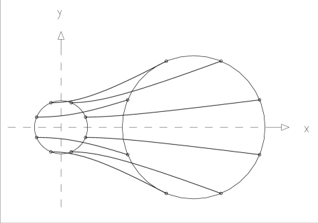
Figure 3: The expectation value of a free three-dimensional spherically symmetric Gaussian wave packet, which initially (at time $t=0$) is at the origin, moves in the positive $x$ direction. As initial volume $V_{0}$ comprising the probability $P$ a sphere around the origin is chosen. Quantile trajectories $\mathchoice{\mbox{\boldmath$\displaystyle\bf x$}}{\mbox{\boldmath$\textstyle\bf x$}}{\mbox{\boldmath$\scriptstyle\bf x$}}{\mbox{\boldmath$\scriptscriptstyle\bf x$}}_{P}(t)$ of points which at $t=0$ lie on the surface of $V_{0}$ at later times lie on the surface of a volume $V_{t}$ which also comprises the same probability $P$. In this simple example all volumes $V_{t}$ are spheres. The plot shows the cuts $z=0$ through two spheres $V_{0},V_{t}$ which are circles and trajectories in the $x,y$ plane.

References

-
[1]
E.H. Hauge and J.A. Støvneng,
Rev. Mod. Phys. 61 (1989) 917.
C.R. Leavens, Tunneling and its Implications, edited by D. Mugnai, A. Ranfagni and L.S. Schulman (World Scientific, Singapore, 1997). - [2] R.S. Dumont, T.L. Marchioro, Phys. Rev. A 47 (1993) 85.
-
[3]
S. Brouard, R. Sala, J.G. Muga, Phys. Rev. A 47
(1994) 4312.
J.G. Muga, S. Brouard, D. Macías, Ann. of Phys. (NY) 240 (1995) 351.
J.G. Muga, V. Delgado, R.F. Snider, Phys. Rev. B 52 (1995) 16381. - [4] A. Challinor, A. Lasenby, S. Somaroo, C. Doran, S. Gull, Phys. Lett. A 227 (1997) 143.
- [5] M.G. Kendall, A. Stuart, The Advanced Theory of Statistics, Vol. 1, 3. ed., Charles Griffin, London 1969.
- [6] S. Brandt, Statistical and Computational Methods in Data Analysis, 2. ed., North Holland, Amsterdam, 1976.
- [7] S. Brandt, H.D. Dahmen, The Picture Book of Quantum Mechanics, 2. ed., Springer-Verlag, New York, 1995.
- [8] E. Gjonaj, Ph.D. Thesis, Universität Siegen, 1998.
-
[9]
D. Bohm, Phys. Rev. 85 (1952) 166; 85 (1952) 180.
D. Bohm, B.J. Hiley and P.N. Kaloyerou, Phys. Rep. 144 No. 6 (1987) 321-375. -
[10]
C.R. Leavens, Solid State Commun. 76 (1990) 253.
C.R. Leavens and G.C. Aers, Solid State Commun. 78 (1991) 1015. - [11] T.P. Spiller, T.D. Clark, R.J. Prance, H. Prance, Europhys. Lett. 12 (1990) 1.
- [12] K. Berndl, Bohmian Mechanics and Quantum Theory. An Appraisal, edited by J.T. Cushing, A. Fine and S. Goldstein (Kluwer, 1996).
- [13] M. Daumer, Bohmian Mechanics and Quantum Theory. An Appraisal, edited by J.T. Cushing, A. Fine and S. Goldstein (Kluwer, 1996).
- [14] W.R. McKinnon and C.R. Leavens, Phys. Rev. A 51 (1995) 2748.
- [15] H. Wu and D.W.L. Sprung, Phys. Lett. A 183 (1993) 413-417.
- [16] C.R. Leavens, Phys. Lett. A 178 (1993) 27.
- [17] P.R. Holland, Phys. Rep. 224 (1993) 95.