FSUJ TPI QO-10a/98

July, 1998

Generation of arbitrary quantum states of traveling fields

M. Dakna, J. Clausen, L. Knöll, and D.-G. Welsch
Friedrich-Schiller-Universität Jena
Theoretisch-Physikalisches Institut
Max-Wien Platz 1, D-07743 Jena, Germany

Abstract

We show that any single-mode quantum state can be generated from the vacuum by alternate application of the coherent displacement operator and the creation operator. We propose an experimental implementation of the scheme for traveling optical fields, which is based on field mixings and conditional measurements in a beam splitter array, and calculate the probability of state generation.

Designing of schemes for the generation of specific nonclassical quantum states has been a subject of increasing interest. The realization in the laboratory of schemes that have been already proposed has been one of the most exciting challenges to the researchers. In [1] a method is proposed that offers the possibility of preparing a cavity-field mode undergoing a Jaynes-Cummings dynamics in any superposition of a finite number of Fock states in principle. The method is based on a non-unitary “collapse” of the state vector of the cavity-field mode via atom ground-state measurement. Before entering the cavity and interacting with the cavity mode in a controlled way, the atoms are prepared in a well-defined superposition of two (Rydberg-)states. After leaving the cavity, the atoms enter a detector for measuring their energies.

In this article we propose a scheme for the preparation of a radiation-field mode in an arbitrary (finite) superposition of Fock states, by performing alternately coherent quantum-state displacement and single-photon adding in a well-defined succession. The advantage of the scheme is that it not only applies to cavity-field modes but also to traveling-field modes. To be more specific, we first recall that coherent quantum-state displacement can be realized for both cavity-field modes (see, e.g., [2]) and traveling-field modes (see, e.g., [3]). In the former case an external (classical) oscillator is resonantly coupled through one of the mirrors to the cavity-field mode. In the latter case the coherent displacement can be achieved with an appropriately chosen beam splitter for mixing the signal mode with a strong local oscillator. With regard to cavity-field modes, single-photon adding can be realized by injecting excited atoms into a cavity and detecting the ground state of the atoms, after leaving the cavity. Adopting the Jaynes-Cummings model, it can be shown [4] that if an atom after interaction with a cavity-field mode is detected in the ground state, then the state of the cavity-field mode is reduced, under certain conditions, to $\sim\hat{a}^{\dagger}|\Phi\rangle$, $|\Phi\rangle$ being the state of the cavity-field mode before the atom enters the cavity. With regard to traveling-field modes, the non-unitary “collapse” to a photon-added state can be realized by conditional output measurement on a beam splitter [5]. In particular, when a mode prepared in a state $|\Phi\rangle$ is mixed at the beam splitter with a single-photon Fock state [6] and a zero-photon measurement is performed in one of the output channels of the beam splitter, then the quantum state of the mode in the other output channels “collapses” to $\sim\hat{Y}|\Phi\rangle$, with

$$\hat{Y}=R\,\hat{a}^{\dagger}T^{\hat{n}}$$ (1)

($R$, reflectance; $T$ transmittance of the beam splitter).

Let us assume that the quantum state that is desired to be generated is a finite superposition of Fock states,

$$|\Psi\rangle=\sum_{n=0}^{N}\psi_{n}\,|n\rangle.$$ (2)

Note that the expansion of any physical state in the Fock basis can always be approximated to any desired degree of accuracy by truncating it at $N$ if $N$ is suitably large. Recalling the definition of Fock states, Eq. (2) can be given by

$$|\Psi\rangle=\sum_{n=0}^{N}\frac{\psi_{n}}{\sqrt{n!}}\,(\hat{a}^{\dagger})^{n}\,|0\rangle,$$ (3)

which may be rewritten as

$$|\Psi\rangle\sim(\hat{a}^{\dagger}\!-\!\beta_{N}^{\ast})(\hat{a}^{\dagger}\!-\!\beta_{N-1}^{\ast})\cdots(\hat{a}^{\dagger}\!-\!\beta_{2}^{\ast})(\hat{a}^{\dagger}\!-\!\beta_{1}^{\ast})\,|0\rangle.$$ (4)

Here, $\beta_{1}^{\ast},\beta_{2}^{\ast},\cdots,\beta_{N}^{\ast}$ are the $N$ (complex) roots of the characteristic polynomial

$$\sum_{n=0}^{N}\frac{\psi_{n}}{\sqrt{n!}}\,(\beta^{\ast})^{n}=0.$$ (5)

Using the relation

$$\hat{a}^{\dagger}\!-\!\beta^{\ast}\!=\!\hat{D}(\beta)\hat{a}^{\dagger}\hat{D}^{\dagger}(\beta),$$ (6)

where $\hat{D}(\beta)$ $\!=$ $\!\exp(\beta\hat{a}^{\dagger}$ $\!-$ $\!\beta^{\ast}\hat{a})$ is the coherent displacement operator, from Eq. (4) we find that

$$|\Psi\rangle\sim\hat{D}(\beta_{N})\hat{a}^{\dagger}\hat{D}^{\dagger}(\beta_{N})$$ (7)

$$\hskip 8.61108pt\times\,\hat{D}(\beta_{N-1})\hat{a}^{\dagger}\hat{D}^{\dagger}(\beta_{N-1})\cdots\hat{D}(\beta_{1})\hat{a}^{\dagger}\hat{D}^{\dagger}(\beta_{1})\,|0\rangle.$$

Hence, any quantum state of the form (2) can be obtained from the vacuum by a succession of alternate state displacement and single-photon adding, the displacements being determined by the roots of the characteristic polynomial (5).

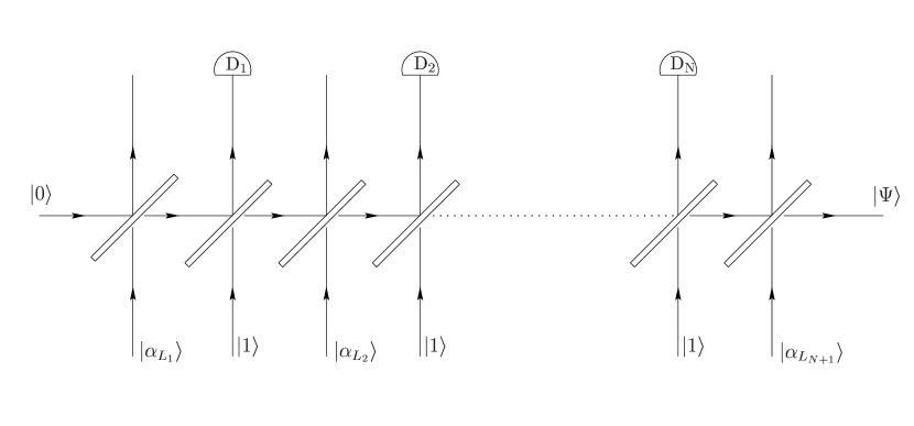
Figure 1: Experimental setup for preparing a traveling-field mode in a quantum state $|\Psi\rangle$, Eq. (2). At the first stage, a mode prepared in the vacuum state $|0\rangle$ and a mode prepared in a strong coherent state $|\alpha_{L_{1}}\rangle$ are superimposed by a beam splitter with transmittance $\tilde{T}$ and reflectance $\tilde{R}$ ($|\tilde{T}|$ $\!\to$ $\!1$) in order to produce a displaced vacuum state $\hat{D}(\alpha_{1})|0\rangle$ with $\alpha_{1}$ $\!=$ $\!\tilde{R}\alpha_{L_{1}}$. At the second stage, the mode prepared in the displaced vacuum state $\hat{D}(\alpha_{1})|0\rangle$ and a mode prepared in a single-photon Fock state $|1\rangle$ are superimposed by a beam splitter with transmittance $T$. When the detector D₁ does not register photons, then the mode in the other output channel of the beam splitter is prepared in a photon-added state $\sim\hat{a}^{\dagger}\,T^{\hat{n}}\hat{D}(\alpha_{1})\,|0\rangle$. Now the two-step procedure is repeated, with the states $\hat{a}^{\dagger}T^{\hat{n}}\hat{D}(\alpha_{1})\,|0\rangle$ and $|\alpha_{L_{2}}\rangle$ in place of the states $|0\rangle$ and $|\alpha_{L_{1}}\rangle$, respectively. As a result, the state $\sim\hat{a}^{\dagger}T^{\hat{n}}\hat{D}(\alpha_{2})\hat{a}^{\dagger}T^{\hat{n}}\hat{D}(\alpha_{1})\,|0\rangle$ is produced. Repeating the procedure $N$ times and performing eventually an additional state displacement $\hat{D}(\alpha_{N+1})$ obviously yields the state in Eq. (8). Choosing the values of $\alpha_{L_{k}}$ such that the values $\alpha_{k}$ in Eqs. (12) – (14) are realized, then the output state $|\Psi\rangle$ is the desired state.

An implementation of the method for a single-mode traveling field is outlined in Fig. 1. Following [5], the state that is produced if no photons are registered in each of the $N$ conditional output measurements is given by

$$|\Psi\rangle\sim\hat{D}(\alpha_{N+1})\hat{a}^{\dagger}T^{\hat{n}}\hat{D}(\alpha_{N})$$ (8)

$$\hskip 25.83325pt\times\,\hat{a}^{\dagger}T^{\hat{n}}\hat{D}(\alpha_{N-1})\cdots\hat{a}^{\dagger}T^{\hat{n}}\hat{D}(\alpha_{1})\,|0\rangle.$$

In order to bring Eq. (8) into the form of Eq. (7), we first write ($k$ $\!=$ $\!1,2,\ldots,N$)

$$T^{\hat{n}}\hat{D}(\alpha_{k})=\hat{D}(\alpha_{k})\left[\hat{D}^{\dagger}(\alpha_{k})T^{\hat{n}}\hat{D}(\alpha_{k})\right]$$ (9)

and then move the operators $\hat{D}^{\dagger}(\alpha_{k})T^{\hat{n}}\hat{D}(\alpha_{k})$ towards the right, on using the relation

$$\left[\hat{D}^{\dagger}(\alpha)T^{\hat{n}}\hat{D}(\alpha)\right]\hat{a}^{\dagger}\!=\!T(\hat{a}^{\dagger}\!+\!\bar{T}\alpha^{\ast})\left[\hat{D}^{\dagger}(\alpha)T^{\hat{n}}\hat{D}(\alpha)\right]$$ (10)

$$\hskip 21.52771pt=T\hat{D}^{\dagger}(\bar{T}^{\ast}\alpha)\,\hat{a}^{\dagger}\,\hat{D}(\bar{T}^{\ast}\alpha)\left[\hat{D}^{\dagger}(\alpha)T^{\hat{n}}\hat{D}(\alpha)\right],$$

where $\bar{T}$ $\!=$ $\!1$ $\!-$ $\!T^{-1}$. After some algebra we obtain

$$|\Psi\rangle\sim\hat{D}(\alpha_{N+1})\,\hat{a}^{\dagger}\hat{D}(T^{*}{}^{-1}\alpha_{N})$$ (11)

$$\hskip 4.30554pt\times\,\hat{a}^{\dagger}\hat{D}(T^{*}{}^{-2}\alpha_{N-1})\cdots\hat{a}^{\dagger}\hat{D}(T^{*}{}^{1-N}\alpha_{2})$$

$$\hskip 4.30554pt\times\,\hat{a}^{\dagger}\hat{D}\!\left(T^{N}\alpha_{1}+\sum_{l=1}^{N}[1\!-\!|T|^{2(l-N)}]T^{N-l}\alpha_{l+1}\right)|0\rangle.$$

Comparing Eqs.(7) and (11), we find that the two equations become identical, if the experimental displacement parameters $\alpha_{k}$ are chosen as follows:

$$\alpha_{1}=-\sum_{l=1}^{N}T^{-l}\alpha_{l+1}\,,$$ (12)

$$\alpha_{k}=T^{\ast}{{}^{N-k+1}}(\beta_{k-1}-\beta_{k})\,,\quad k=2,3,\ldots,N,$$ (13)

$$\alpha_{N+1}=\beta_{N}\,.$$ (14)

The numerical implementation of the method is rather simple. First the roots of the polynomial (5) are calculated, which can be done using standard routines. A straightforward calculation then yields, according to Eqs. (12) – (14), the displacement parameters required in the experimental scheme.

Let us address the question of what is the probability $P_{|\Psi\rangle}$ of producing a chosen state $|\Psi\rangle$. Obviously, this probability is determined by the requirement that all the $N$ detectors do not register photons. It can be given by

$$P_{|\Psi\rangle}=P(N,0|1,0;2,0;\ldots;N\!-\!1,0)\cdots$$ (15)

$$\hskip 34.44434pt\times\cdots P(2,0|1,0)\,P(1,0).$$

Here, $P(k,0|1,0;2,0;\ldots;k\!-\!1,0)$ is the probability that the $k$th detector does not register photons under the condition that the detectors D₁,D₂,…,D_k-1 have also not registered photons. To calculate the conditional probabilities in Eq. (15), we note that the $k$th zero-photon measurement corresponds to the application of the operator $\hat{Y}$, Eq. (1), to the state resulting from the $(k\!-\!1)$th zero-photon measurement (and subsequent displacement). Starting from

$$P(1,0)=\|\hat{Y}\hat{D}(\alpha_{1})|0\rangle\|^{2},$$ (16)

we derive step by step ($k$ $\!=$ $\!2,3,\ldots,N$)

$$P(k,0|1,0;2,0;\ldots;k\!-\!1,0)$$ (17)

$$\hskip 8.61108pt=\frac{\|\hat{Y}\hat{D}(\alpha_{k})\hat{Y}\hat{D}(\alpha_{k-1})\cdots\hat{Y}\hat{D}(\alpha_{1})|0\rangle\|^{2}}{\|\hat{Y}\hat{D}(\alpha_{k-1})\cdots\hat{Y}\hat{D}(\alpha_{1})|0\rangle\|^{2}}$$

($\|\,|\Phi\rangle\|$ $\!=$ $\!\sqrt{\langle\Phi|\Phi\rangle}$). Combining Eqs. (15) and (17), we find that

$$P_{|\Psi\rangle}={\cal P}_{N}^{2},$$ (18)

where

$${\cal P}_{k} = \|\hat{Y}\hat{D}(\alpha_{k})\hat{Y}\hat{D}(\alpha_{k-1})\cdots\hat{Y}\hat{D}(\alpha_{1})|0\rangle\|.$$ (19)

Substituting in Eq. (19) for $\hat{Y}$ Eq. (1) and using Eqs. (9), (10), and (6), after some algebra we obtain

$${\cal P}_{k}^{2}=|R|^{2k}|T|^{k(k-1)}\bigg{\|}\prod_{m=1}^{k}\left(\hat{a}^{\dagger}\!+\!b_{mk}^{\ast}\right)|\gamma_{k}\rangle\bigg{\|}^{2}$$ (20)

$$\hskip 25.83325pt\times\,\exp\!\left(-|R|^{2}\sum_{m=1}^{k}\bigg{|}\sum_{j=1}^{m}T^{m-j}\alpha_{j}\bigg{|}^{2}\right)$$

where the abbreviations $b_{1k}$ $\!=$ $\!0$,

$$b_{mk}=-\sum_{j=0}^{m-2}T^{\ast}{{}^{-j-1}}\alpha_{k-j}\,,\quad m=2,3,\ldots,k,$$ (21)

and

$$\gamma_{k}=\sum_{j=1}^{k}T^{k+1-j}\alpha_{j}$$ (22)

have been introduced. To calculate the square of the norm of the state in Eq. (20), we may write

$$\bigg{\|}\prod_{m=1}^{k}(\hat{a}^{\dagger}\!+\!b_{mk}^{\ast})|\gamma_{k}\rangle\bigg{\|}^{2}$$ (23)

$$\hskip 4.30554pt=\langle\gamma_{k}|\prod_{m=1}^{k}(\hat{a}\!+\!b_{mk})\prod_{l=1}^{k}(\hat{a}^{\dagger}\!+\!b_{lk}^{\ast})|\gamma_{k}\rangle$$

$$\hskip 4.30554pt=\sum_{m,l=0}^{k}\bigg{\{}\bigg{[}\sum_{i_{1},\cdots,i_{m}}{{}^{{}^{{}^{<}}}}b_{i_{1}k}\cdots b_{i_{m}k}\bigg{]}\bigg{[}\sum_{i_{1},\cdots,i_{l}}{{}^{{}^{{}^{<}}}}b_{i_{1}k}^{\ast}\cdots b_{i_{l}k}^{\ast}\bigg{]}$$

$$\hskip 86.11084pt\times\,\langle\gamma_{k}|\hat{a}^{k-m}\hat{a}^{\dagger}{{}^{k-l}}|\gamma_{k}\rangle\bigg{\}},$$

where the symbol $\sum_{i_{1},i_{2},\cdots}{{}^{{}^{{}^{<}}}}\hskip 21.52771pt$ is used to indicate that the summation requires the condition $i_{1}$ $\!<$ $\!i_{2}$ $\!<$ $\!\cdots$ to be satisfied, and

$$\langle\gamma_{k}|\hat{a}^{k-m}\hat{a}^{\dagger}{{}^{k-l}}|\gamma_{k}\rangle$$ (26)

$$\hskip 8.61108pt=\left\{\begin{array}[]{ll}(k\!-\!m)!\gamma_{k}^{\ast}{{}^{m-l}}{\rm L}_{k-m}^{m-l}\big{(}-|\gamma_{k}|^{2}\big{)}&\ \mbox{if}\quad l<m,\\[8.61108pt] (k\!-\!l)!\gamma_{k}^{l-m}{\rm L}_{k-l}^{l-m}\big{(}-|\gamma_{k}|^{2}\big{)}&\ \mbox{if}\quad l\geq m\end{array}\right.$$

[L${}_{n}^{m}(x)$ being the generalized Laguerre polynomial].

In order to illustrate the method, let us consider the generation of truncated coherent phase states [7]

$$|\Psi\rangle\equiv|z;N\rangle=C(z;N)\sum_{n=0}^{N}z^{n}\,|n\rangle,$$ (27)

where

$$C(z;N)=\left\{\begin{array}[]{ll}\displaystyle\sqrt{\frac{1\!-\!|z|^{2}}{1\!-\!|z|^{2(N+1)}}}&\ {\rm if}\ |z|<1,\\[4.30554pt] \displaystyle\frac{1}{\sqrt{N+1}}&\ {\rm if}\ |z|=1.\end{array}\right.$$ (30)

The roots $\beta_{k}^{\ast}$ of the characteristic polynomial

$$\sum_{n=0}^{N}\frac{z^{n}}{\sqrt{n!}}\,(\beta^{\ast})^{n}=0$$ (31)

are given in Tab. 1 for $z$ $\!=$ $\!0.4$ and $N$ $\!=$ $\!6$. The table also shows the values of the displacement parameters $\alpha_{k}$ calculated from Eqs. (12) – (14) for $T$ $\!=$ $\!0.99$. The probability of producing the state is $P_{|\Psi\rangle}$ $\!=$ $\!0.02\%$. For chosen state the probability $P_{|\Psi\rangle}$ sensitively depends on the absolute value of the transmittance of the beam splitter, $|T|$, as it can be seen from Fig. 2 for two truncated coherent phase states. The probability increases with $|T|$, attains a maximum, and then rapidly approaches zero as $|T|$ goes to unity. So far we have assumed that the beam splitters used for photon adding have the same transmittance. Assuming different beam splitters, one may ask for the optimum set of transmittances that gives the highest probability of producing a chosen state. Our numerical calculations for the truncated coherent phase states has not led to a substantial improvement compared to the case when equal beam splitters are used.

In summary, we have shown that single-mode radiation can be prepared in arbitrary pure quantum states, by a succession of alternate state displacement and single-photon adding. With regard to traveling fields, these operations can be realized within a beam-splitter array into which coherent states and single-photon Fock states are fed and zero-photon measurements are performed using highly efficient avalanche photodiodes. It is worth noting that the generation of arbitrary pure quantum states of traveling fields offers new possibilities of quantum-state measurement, such as projection synthesis for measuring the overlaps $|\langle A|\Phi\rangle|^{2}$ of a given state $|\Phi\rangle$ with arbitrary states $|A\rangle$ [8, 9]. Projection synthesis simply uses a beam splitter for combining the signal mode prepared in the state $|\Phi\rangle$ and a reference mode prepared in a state $|\Psi\rangle$ and two photodetectors in the output channels of the beam splitter for measuring the joint-event probability distribution. The states $|\Psi\rangle$ can be calculated from the states $|A\rangle$ (e.g., the states $|\Psi\rangle$ that are associated with the truncated phase states are reciprocal binomial states [8]). Obviously, the crucial point is the preparation of specific states $|\Psi\rangle$, which may be solved using the method proposed here.

Note added. After preparing the article we were made aware of a paper on the preparation of a superposition of the vacuum and one-photon states of traveling fields by using similar basic elements [10].

Table 1: The roots $\beta_{k}^{\ast}$ $\!=$ $|\beta_{k}|e^{-i\varphi_{\beta_{k}}}$ of the characteristic polynomial (31) and the displacement parameters $\alpha_{k}$ $\!=$ $|\alpha_{k}|e^{i\varphi_{\alpha_{k}}}$, Eqs. (12) – (14), are given for a truncated coherent phase state $|\Psi$ $\!=$ $|z;N\rangle$ ($z$ $\!=$ $\!0.4$, $N$ $\!=$ $\!6$), and $T$ $\!=$ $\!0.99$. The probability of producing the state is $P_{|\Psi\rangle}$ $\!=$ $\!0.02\%$. It is calculated from Eq. (18), the values of the ${\cal P}_{k}^{2}$ are given in the last column.

Figure 2: The probability $P_{|\Psi\rangle}$ of producing truncated coherent phase states $|\Psi\rangle$ $\!=$ $|z;N\rangle$, Eq. (27), is shown as a function of the absolute value of the beam-splitter transmittance $|T|$ for $N$ $\!=$ $\!6$ (solid line) and $N$ $\!=$ $\!5$ (dotted line), and $z$ $\!=$ $\!0.4$. It is assumed that the beam splitters used for photon adding have the same transmittance.

References

• [1] K. Vogel, V.M. Akulin, and W.P. Schleich, Phys. Rev. Lett. 71, 1816 (1993).
• [2] P. Alsing, D.-S. Guo, and H.J. Carmichael, Phys. Rev. A 45, 5135 (1992).
• [3] M.G.A. Paris, Phys. Lett. A 217, (1996); M. Ban, J. Mod. Opt. 44, 1175 (1997).
• [4] G.S. Agarwal and K. Tara, Phys. Rev. A 43, 492 (1991).
• [5] M. Dakna, L. Knöll, and D.-G. Welsch, Opt. Commun. 145, 309 (1998); D.-G. Welsch, M. Dakna, L. Knöll, and T. Opatrný, in Proceedings of the 5th International Conference on Squeezed States and Uncertainty Relations (Balatonfüred, 1997), edited by D. Han, J. Janszky, Y.S. Kim, V.I. Man’ko (NASA/CP-1998-206855, Greenbelt, 1998) p. 609.
• [6] Single-photon Fock states can be produced using parametric down conversion, in which correlated photon pairs are emitted and one of the photons is used for timing and control of the other [C.K. Hong and L. Mandel, Phys. Rev. Lett. 56, 58 (1986)]. They have been used in various experiments [see, e.g., P. Kwiat, K. Mattle, H. Weinfurter, A. Zeilinger, A. Sergienko, and Y. Shih, Phys. Rev. Lett. 75, 4437 (1995); J. G. Rarity, P. R. Tapster, and R. Loudon, quant-ph/9702032.
• [7] J.M. Lèvy-Leblond, Ann. Phys. 101, 319 (1976); J.H. Shapiro and S. R. Shepard, Phys. Rev. A 43, 3795 (1991).
• [8] S.M. Barnett and D.T. Pegg, Phys. Rev. Lett 76, 4148 (1996).
• [9] B. Baseia, M.H.Y Moussa, and V.S Bagnato, Phys. Lett. A 231, 331 (1997).
• [10] D.T. Pegg, L.S. Phillips, and S.M. Barnett, Phys. Rev. Lett 81, 1604 (1998).
Refer to caption