Heisenberg picture operators in the quantum state diffusion model

Abstract

A stochastic simulation algorithm for the computation of multitime correlation functions which is based on the quantum state diffusion model of open systems is developed. The crucial point of the proposed scheme is a suitable extension of the quantum master equation to a doubled Hilbert space which is then unraveled by a stochastic differential equation.

Within the framework of the recently developed stochastic wave function approach to open quantum systems [1, 2, 3, 4, 5, 6, 7, 8] the state of a system is not described by a reduced density matrix but by a pure stochastic state vector $\psi_{t}$ whose covariance matrix is equal to the reduced density matrix of the system. One of these models which was motivated by a dynamical description of the measurement process [9] is the quantum state diffusion model introduced by Gisin and Percival [5, 6]. In this approach, the time-evolution of the wave function $\psi_{t}$ is governed by the Ito stochastic differential equation

$$d\psi_{t}= - \mathrm{i}{H}\psi_{t}dt+\frac{1}{2}\sum_{j}\left[2\langle{L}_{j}^{\dagger}\rangle_{\psi_{t}}{L}_{j}-{L}_{j}^{\dagger}{L}_{j}-\langle{L}_{j}\rangle_{\psi_{t}}\langle{L}_{j}^{\dagger}\rangle_{\psi_{t}}\right]\psi_{t}dt$$ (1)

$$+ \sum_{j}\left[{L}_{j}-\langle{L}_{j}\rangle_{\psi_{t}}\right]\psi_{t}d\xi_{jt},$$

where $\langle{L}_{j}\rangle_{\psi_{t}}$ is a short-hand notation for $\langle\psi_{t}|{L}|\psi_{t}\rangle$, and $d\xi_{jt}$ is the differential of a complex valued Wiener process with means and correlations

$$\langle d\xi_{jt}\rangle=\langle d\xi_{it}d\xi_{jt}\rangle=0,\quad\langle d\xi_{it}d\xi_{jt}^{*}\rangle=\delta_{ij}dt.$$ (2)

The operators $H$ and $L_{j}$ acting in the Hilbert space $\mathcal{H}$ of the system are the free Hamiltonian and the Lindblad operators describing dissipation, respectively. The link to the density matrix description of open quantum systems is established – as mentioned above – through the covariance matrix of the stochastic wave function $\psi_{t}$, i. e.,

$$\rho_{t}=\mathrm{E}\left(|\psi_{t}\rangle\langle\psi_{t}|\right).$$ (3)

The symbol E denotes the expectation value with respect of the stochastic processes $\psi_{t}$. The equation of motion of the density matrix $\rho_{t}$ is obtained by inserting eq. (1) in eq. (3) which yields the quantum master equation

$$\dot{\rho}(t)=-{\mathrm{i}}\left[H,\rho(t)\right]+\frac{1}{2}\sum_{j}\left[2L_{j}\rho(t)L_{j}^{\dagger}-L_{j}^{\dagger}L_{j}\rho(t)-\rho(t)L_{j}^{\dagger}L_{j}\right].$$ (4)

This equation – or alternatively the stochastic differential equation (1) – determines the time-evolution of one-time expectation values of system observables. Multitime correlation functions which are of special interest in quantum optics or in solid state physics are not specified by these equations. In order to define these quantities, we will first define the matrix elements of some system operator $A$ in the Heisenberg picture. In the density matrix approach, these matrix elements are defined through the quantum regression theorem [10, 11] as

$$A_{t}(\phi_{0},\psi_{0})\equiv\langle\phi_{0},t_{0}|A(t)|\psi_{0},t_{0}\rangle=\mbox{Tr}\Big{\{}AV(t,t_{0})\left\{|\psi_{0}\rangle\langle\phi_{0}|\right\}\Big{\}},$$ (5)

where $V(t,t_{0})$ is the time-evolution superoperator corresponding to the quantum master equation (4). Unfortunately, the quantum regression theorem cannot be applied directly to the stochastic wave function approach, since the initial “density matrix” $|\psi_{0}\rangle\langle\phi_{0}|$ is not necessarily Hermitian, and hence it can in general not be the covariance matrix of some stochastic wave function. This problem can be resolved by extending the quantum master equation into a doubled Hilbert space $\tilde{\mathcal{H}}={\mathcal{H}}\oplus{\mathcal{H}}$ in the following way: we define a density matrix $\widetilde{\rho}(t)$ as

$$\widetilde{\rho}(t)=\left(\begin{array}[]{cc}\widetilde{\rho}_{11}(t)&\widetilde{\rho}_{12}(t)\\ \widetilde{\rho}_{21}(t)&\widetilde{\rho}_{22}(t)\end{array}\right),$$ (6)

where $\widetilde{\rho}_{ij}(t)$ are operators on ${\mathcal{H}}$ and accordingly replace the Hamiltonian $H$ and the Lindblad operators $L_{j}$ by the operators

$$\widetilde{H}=\left(\begin{array}[]{cc}H&0\\ 0&H\end{array}\right),\quad\widetilde{L}_{j}=\left(\begin{array}[]{cc}L_{j}&0\\ 0&L_{j}\end{array}\right)$$ (7)

in the doubled Hilbert space $\widetilde{\mathcal{H}}$. Then we formulate the extended quantum master equation

$$\dot{\widetilde{\rho}}(t)=-\mathrm{i}\left[\widetilde{H},\widetilde{\rho}(t)\right]+\frac{1}{2}\sum_{j}\left[2\widetilde{L}_{j}\widetilde{\rho}(t)\widetilde{L}_{j}^{\dagger}-\widetilde{L}_{j}^{\dagger}\widetilde{L}_{j}\widetilde{\rho}(t)-\widetilde{\rho}(t)\widetilde{L}_{j}^{\dagger}\widetilde{L}_{j}\right].$$ (8)

The crucial point of this construction is that each element $\widetilde{\rho}_{ij}(t)$ of the density matrix $\widetilde{\rho}(t)$ is a solution of the original quantum master equation (4). Consider now the initial condition

$$\widetilde{\rho}(t_{0})=|\theta_{0}\rangle\langle\theta_{0}|\equiv\frac{1}{2}\left(\begin{array}[]{cc}|\phi_{0}\rangle\langle\phi_{0}|&|\phi_{0}\rangle\langle\psi_{0}|\\ |\psi_{0}\rangle\langle\phi_{0}|&|\psi_{0}\rangle\langle\psi_{0}|\end{array}\right),$$ (9)

where $\theta_{0}\equiv(\phi_{0},\psi_{0})^{\mathrm{T}}/\sqrt{2}$ is an element of the doubled Hilbert space $\widetilde{\mathcal{H}}$. (Throughout this letter the superscript ${\mathrm{T}}$ denotes the transpose). Obviously, the matrix elements of some operator $A$ are then given by

$$A_{t}(\phi_{0},\psi_{0})=2\mbox{Tr}\Big{\{}A\widetilde{\rho}_{21}(t)\Big{\}}.$$ (10)

By construction, the initial density matrix $\widetilde{\rho}(t_{0})=|\theta_{0}\rangle\langle\theta_{0}|$ is positive and we may choose any unraveling of the extended quantum master equation (8) by a stochastic process for the calculation of its time-evolution and hence for the calculation of operators in the Heisenberg picture (A similar idea has been proposed in Ref. [4] Appendix D).

Applying the above procedure to the quantum state diffusion model we obtain for example the equation of motion for the wave function $\theta_{t}=(\phi_{t},\psi_{t})^{\mathrm{T}}\in\widetilde{\mathcal{H}}$ in the Ito form

$$d\theta_{t}= - \mathrm{i}\widetilde{H}\theta_{t}dt+\frac{1}{2}\sum_{j}\left[2\langle\widetilde{L}_{j}^{\dagger}\rangle_{\theta_{t}}\widetilde{L}_{j}-\widetilde{L}_{j}^{\dagger}\widetilde{L}_{j}-\langle\widetilde{L}_{j}\rangle_{\theta_{t}}\langle\widetilde{L}_{j}^{\dagger}\rangle_{\theta_{t}}\right]\theta_{t}dt$$ (11)

$$+ \sum_{j}\left[\widetilde{L}-\langle\widetilde{L}_{j}\rangle_{\theta_{t}}\right]\theta_{t}d\xi_{jt}.$$

The matrix elements of $A$ are simply obtained as

$$A_{t}(\phi_{0},\psi_{0})=2\mathrm{E}_{\theta_{0}}(\langle\phi_{t}|A|\psi_{t}\rangle),$$ (12)

where $\mathrm{E}_{\theta_{0}}$ denotes the expectation value with respect to the initial condition $\theta_{0}$. Note, that eq. (11) is constructed in such a way that the norm of the state vector $\theta_{t}$ is preserved, i. e., $||\theta_{t}||^{2}=||\phi_{t}||^{2}+||\psi_{t}||^{2}=1$. From a numerical point of view it is more efficient to drop this restriction and to work with unnormalized state vectors $\hat{\theta}_{t}$, whose time-evolution is governed by the quasi-linear stochastic differential equation [5]

$$d\hat{\theta}_{t}=-\mathrm{i}\widetilde{H}\hat{\theta}_{t}dt+\sum_{j}\widetilde{L}_{j}\hat{\theta}_{t}\left(d\xi_{jt}+\langle\widetilde{L}_{j}^{\dagger}\rangle_{\theta_{t}}dt\right)-\frac{1}{2}\sum_{j}\widetilde{L}_{j}^{\dagger}\widetilde{L}_{j}\hat{\theta}_{t}dt.$$ (13)

Accordingly, the matrix elements of the operator $A$ are defined as

$$A_{t}(\phi_{0},\psi_{0})=2E_{\theta_{0}}\left(\langle\hat{\phi}_{t}|A|\hat{\psi}_{t}\rangle/||\hat{\theta}_{t}||^{2}\right).$$ (14)

As a particular example, we consider a two-level system with $H=0$ coupled to the vacuum using the Lindblad operator $\sigma^{-}$, and calculate the matrix element $\langle\phi_{0}|\sigma^{+}(t)|\psi_{0}\rangle$, where $\phi_{0}=(1,0)^{\mathrm{T}}$ and $\psi_{0}=(1,1)^{\mathrm{T}}/\sqrt{2}$. The analytical solution

$$\langle\phi_{0}|\sigma^{+}(t)|\psi_{0}\rangle=\frac{1}{\sqrt{2}}e^{-t/2}$$ (15)

is readily obtained by integrating the quantum master equation. In Fig.1 we compare the numerical solution obtained using the scheme described above for $10^{3}$ realizations (diamonds) with the analytical solution (thick line). Obviously, both solutions are in excellent agreement.

Alternatively, Gisin proposes in Ref. [13] a similar scheme for the calculation of matrix elements which is based on the coupled system of stochastic differential equations

$$d\psi_{t}=-\mathrm{i}H\psi_{t}dt+\frac{1}{2}\sum_{j}\left[2l_{j}(\psi_{t},\phi_{t})^{*}L_{j}-L_{j}^{\dagger}L_{j}-l_{j}(\phi_{t},\psi_{t})l_{j}(\psi_{t},\phi_{t})^{*}\right]\psi_{t}dt$$

$$+ \sum_{j}\left[L-l_{j}(\phi_{t},\psi_{t})\right]\psi_{t}d\xi_{jt},$$

$$d\phi_{t}=-\mathrm{i}H\phi_{t}dt+\frac{1}{2}\sum_{j}\left[2l_{j}(\phi_{t},\psi_{t})^{*}L_{j}-L_{j}^{\dagger}L_{j}-l_{j}(\psi_{t},\phi_{t})l_{j}(\phi_{t},\psi_{t})^{*}\right]\phi_{t}dt$$ (16)

$$+ \sum_{j}\left[L-l_{j}(\psi_{t},\phi_{t})\right]\phi_{t}d\xi_{jt},$$

where $l_{j}(\alpha,\beta)=\langle\alpha|L_{j}|\beta\rangle/\langle\alpha|\beta\rangle$. These equations are constructed in such a way that the scalar product $\langle\phi_{t}|\psi_{t}\rangle$ remains constant during the time-evolution of the system, i. e., the matrix element of the unity operator $I_{t}=I$ are calculated correctly for each realization of the stochastic process (and not only in the mean). In addition, he also proposes in Ref. [13] a pair of quasi-linear equations, which could be used for the numerical simulation. However, although the above equations correctly reproduce the equation of motion for the matrix elements, the numerical integration of the stochastic differential equations for the system described above, suggests that these equations are not stable in general. In order to demonstrate this, we have also plotted in Fig. 1 the numerical solution of the quasi-linear stochastic differential equations for various step-sizes ($h=0.01,0.001,0.0001$) and $10^{4}$ realization each. The systematic deviation of the numerical and analytical solutions for $t\gtrsim 0.3\gamma^{-1}$ is evident. We believe, that these deviations are due to the fact, that the solution of the deterministic part of the stochastic differential equation is unstable for this particular model which leads to immense fluctuations in the solution of the stochastic differential equation. Note, that the fluctuations are even much larger for the integration of the “unity-preserving” equation (Heisenberg picture operators in the quantum state diffusion model).

The simulation algorithm in the doubled Hilbert space for the calculation of matrix elements in the Heisenberg picture is the basis for the computation of multitime correlation functions such as $g(t,t+\tau)=\langle\psi_{0}|A(t+\tau)B(t)|\psi_{0}\rangle$ and we propose the following procedure: start in the state $\psi_{0}$ and propagate it up to the time $t$ using the stochastic differential equation (1) to obtain $\psi_{t}$. Define the state vector $\theta_{t}=(\psi_{t},B\psi_{t})^{\mathrm{T}}/\sqrt{1+||B\psi_{t}||^{2}}$ and propagate it up to the time $t+\tau$ by integrating the extended stochastic differential equation (11). The two-time correlation function $g(t,t+\tau)$ is then given by

$$g(t,t+\tau)={\mathrm{E}}\left[\left(1+||B\psi_{t}||^{2}\right)\langle\phi_{t+\tau}|A|\psi_{t+\tau}\rangle\right].$$ (17)

As a specific example we have computed the first order correlation function $\langle\sigma^{+}(t+\tau)\sigma^{-}(t)\rangle_{s}$ for a coherently driven two-level atom on resonance in the steady state with Rabi frequency $\Omega=10\gamma$. To this end, we started with a random initial state vector $\psi_{0}$ drawn from a uniform distribution on ${\mathcal{H}}$ and propagated it up to $t=30\gamma^{-1}$ in order to reach the steady state regime. Then we proceeded as described above. The result of the numerical simulation is shown in Fig. 2 (a) for $10^{4}$ realizations. The numerical performance of the algorithm is demonstrated in Fig. 2 (b) where we have plotted the computational time which is necessary to obtain a given accuracy measured by the relative mean square error (solid line) and the estimated standard deviation of the samples (dashed line). These results are compared with an alternative procedure which is based on an unraveling of the extended quantum master equation by a piecewise deterministic jump process (see Ref. [12]). The algorithm based on quantum jumps is about two times faster than the one based on the quantum state diffusion model. At a first glance, this result is surprising, since the individual realizations of the diffusion process are smooth and “closer” to the real solution. But this is outweighed by the fact that for the integration of the stochastic differential equation we have to draw two random numbers per time step and Lindblad operator, whereas in the quantum jump method we have to generate only two random numbers per jump. Thus, a single realization of the diffusion process is more accurate, but takes longer to be computed.

To summarize, we have shown that operators in the Heisenberg picture and multitime correlation functions can be calculated within the framework of the quantum state diffusion model by extending the stochastic differential equation which governs the time-evolution of the wave function to the doubled Hilbert space. This procedure is in complete agreement with the quantum regression theorem. However, we have also shown that the latter fact is not sufficient to ensure that a particular simulation algorithm is of practical use: Although the algorithm proposed in Ref. [13] is in accordance with the quantum regression theorem, it seems not to be stable in general. On the other hand, the scheme we proposed in this letter completely relies on the numerical stability of the quantum state diffusion model.

References

Figure 1: Calculation of Heisenberg operator matrix element $\langle\phi_{0}|\sigma^{+}(t)|\phi_{0}\rangle$: analytical solution (thick line), numerical solution using the quantum state diffusion unraveling of the extended quantum master equation for $10^{3}$ realizations (diamonds), and the method proposed by Gisin (thin lines) for the step-sizes $h=0.01,0.001,0.0001$.

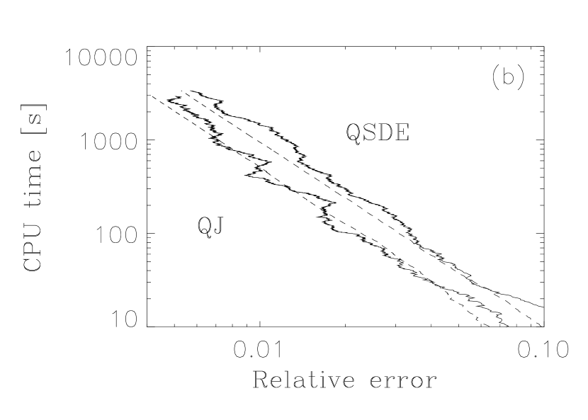
Figure 2: Calculation of the first order correlation function $\langle\sigma^{+}(\tau)\sigma^{-}\rangle_{s}$ for a coherently driven two-level atom on resonance. (a) Analytical solution vs. the numerical solution (diamonds) using the quantum state diffusion model for $10^{4}$ realizations. (b) CPU time in seconds vs. the relative error for the simulation using the quantum state diffusion model (QSDE) and the quantum jump method (QJ). The solid lines represent the mean square deviation of the numerical solution from the exact solution and the dashed lines show the estimated standard deviation of the numerical solution.

References

[1]
J. Dalibard, Y. Castin, and K. Mølmer, Phys. Rev. Lett. 68, 580
(1992).
[2]
H. Carmichael, An Open Systems Approach to Quantum Optics, Lecture
Notes in Physics m18 (Springer-Verlag, Berlin, Heidelberg, New York, 1993).
[3]
C. W. Gardiner, A. S. Parkins, and P. Zoller, Phys. Rev. A 46, 4363
(1992).
[4]
R. Dum, A. S. Parkins, P. Zoller, and C. W. Gardiner, Phys. Rev. A 46,
4382 (1992).
[5]
N. Gisin and I. C. Percival, J. Phys. A 25, 5677 (1992).
[6]
N. Gisin and I. C. Percival, J. Phys. A 26, 2233 (1993).
[7]
H. P. Breuer and F. Petruccione, Phys. Rev. Lett. 74, 3788 (1995).
[8]
H. P. Breuer and F. Petruccione, Phys. Rev. E 52, 428 (1995).
[9]
N. Gisin, Phys. Rev. Lett. 52, 1657 (1984).
[10]
C. W. Gardiner, Quantum Noise (Springer-Verlag, Berlin; Heidelberg, New
York, 1991).
[11]
D. F. Walls and G. J. Milburn, Quantum Optics (Springer-Verlag, Berlin,
Heidelberg, New York, 1994).
[12]
H. P. Breuer, B. Kappler, and F. Petruccione,
Phys. Rev. A 56, 2334 (1997).
[13]
N. Gisin, J. mod. Optics 40, 2313 (1993).