Time-of-Arrival States

Abstract

Although one can show formally that a time-of-arrival operator cannot exist, one can modify the low momentum behaviour of the operator slightly so that it is self-adjoint. We show that such a modification results in the difficulty that the eigenstates are drastically altered. In an eigenstate of the modified time-of-arrival operator, the particle, at the predicted time-of-arrival, is found far away from the point of arrival with probability $1/2$

I Introduction

In quantum mechanics, observables like position and momentum are represented by operators at a fixed time $t$. However, there is no operator associated with the time it takes for a particle to arrive to a fixed location. One can construct such a time-of-arrival operator [1], but its physical meaning is ambiguous [2] [3][4]. In classical mechanics, one can answer the question, "at what time does a particle reach the location $x=0$?", but in quantum mechanics, this question does not appear to have an unambiguous answer. In [3] we proved formally, that in general a time-of-arrival operator cannot exist. This is because one can prove that the existence of a time-of-arrival operator implies the existence of a time operator. As Pauli [5] showed, one cannot have a time operator if the Hamiltonian of the system is bounded from above or below.

There has however been renewed interest in time-of-arrival, following the suggestion by Grot, Rovelli, and Tate, that one can modify the time-of-arrival operator in such away as to make it self-adjoint [6]. The idea is that by modifying the operator in a very small neighbourhood around $k=0$, one can formally construct a modified time-of-arrival operator which behaves in much the same way as the unmodified time-of-arrival operator.

In this paper, we examine the behaviour of the modified time-of-arrival eigenstates, and show that the modification, no matter how small, radically effects the behaviour of the states. We find that the particles in these eigenstates don’t arrive with a probability of $1/2$ at the predicted time-of-arrival.

In Section II we show why the time-of-arrival operator is not self-adjoint, and explore the possible modifications that can be made in order to make it self-adjoint. We then explore some of the properties of the modified time-of-arrival states. In Section III we examine normalizable states which are coherent superpositions of time-of-arrival eigenstates, and discuss the possibility of localizing these states at the location of arrival at the time-of-arrival. These results seem to agree with those of Muga and Leavens who have studied these states independently [7]. Our central result is contained in Section IV where we show that in an eigenstate of the modified time-of-arrival operator, the particle, at the predicted time-of-arrival, is found far away from the point of arrival with probability $1/2$ We also calculate the average energy of the states, in order to relate them to our proposal [3] that one cannot measure the time-of-arrival to an accuracy better than $1/\bar{E}_{k}$ where $\bar{E}_{k}$ is the average kinetic energy of the particle. We finish with some concluding remarks in Section V.

II The Time-of-Arrival Operator

Classically, the position of a free particle is given by

$$x(t)=\frac{p_{o}t}{m}+x_{o}$$ (1)

One can invert this equation to find the time that a particle arrives to a given location. From the correspondence principal, one can then try to define a time-of-arrival operator ${\bf T}$. The time-of-arrival operator to the point $x=0$ can be written in the $k$ representation as

$${\bf T}(k)=-im\frac{1}{\sqrt{k}}\frac{d}{dk}\frac{1}{\sqrt{k}}\,$$ (2)

where $\sqrt{k}=i\sqrt{|k|}$ for $k<0$. It can be verified that the eigenstates of this operator are given by

$$g_{t_{A}}(k)=\alpha(k)\frac{1}{\sqrt{2\pi m}}\sqrt{k}e^{i\frac{t_{A}k^{2}}{2m}}$$ (3)

where $\alpha=\left(\theta(k)+i\theta(-k)\right)$. These eigenstates however, are not orthogonal.

$$\langle t_{A}^{\prime}|t_{A}\rangle = \frac{1}{\sqrt{2\pi m}}\int_{0}^{\infty}dk^{2}\,e^{\frac{i}{2m}k^{2}(t_{A}-t_{A}^{\prime})}$$ (4)

$$= \delta(t_{A}-t_{A}^{\prime})-\frac{i}{\pi(t_{A}-t_{A}^{\prime})}.$$ (5)

The reason for this, is that the adjoint of ${\bf T}$ has a different domain of definition than ${\bf T}$ itself. If ${\bf T}$ is defined over all square integrable, differentiable functions $v(k)$, then the quantity

$$\langle u,{\bf T}v\rangle-\langle{\bf T}^{*}u,v\rangle = -i\,m\int dk\left[\frac{\overline{u(k)}}{\sqrt{k}}\frac{d}{dk}\frac{v(k)}{\sqrt{k}}+v(k)\overline{\frac{1}{\sqrt{k}}\frac{d}{dk}\frac{u(k)}{\sqrt{k}}}\right]$$ (6)

$$= i\,m\int_{-\infty}^{0^{-}}dk\left[\frac{\overline{u(k)}}{\sqrt{|k|}}\frac{d}{dk}\frac{v(k)}{\sqrt{|k|}}+v(k)\overline{\frac{1}{\sqrt{|k|}}\frac{d}{dk}\frac{u(k)}{\sqrt{|k|}}}\right]\,\,-$$ (8)

$$i\,m\int_{0^{+}}^{\infty}dk\left[\frac{\overline{u(k)}}{\sqrt{k}}\frac{d}{dk}\frac{v(k)}{\sqrt{k}}+v(k)\overline{\frac{1}{\sqrt{k}}\frac{d}{dk}\frac{u(k)}{\sqrt{k}}}\right]$$

$$= i\,m\left[\lim_{k\rightarrow 0^{-}}\frac{v(k)\overline{u(k)}}{|k|}+\lim_{k\rightarrow 0^{+}}\frac{v(k)\overline{u(k)}}{|k|}\right]$$ (9)

will only vanish if $\frac{v(k)\overline{u(k)}}{k}$ is continuous through $k=0$. Since $v(k)$ is arbitrary, ${\bf T}^{*}$ is only defined for functions $u(k)$ such that $u(k)/k$ is continuous. On the other hand, if we change the domain of definition of ${\bf T}$ so that it is defined on functions $v(k)$ such that $\frac{v(k)}{\sqrt{k}}$ is continuous through $k=0$, then ${\bf T}^{*}$ will only be defined on functions $u(k)$ such that $\frac{u(k)}{\sqrt{k}}$ is anti-continuous. The domain of definition of ${\bf T}$ and ${\bf T}^{*}$ are different, and thus ${\bf T}$ is not self-adjoint. The problem is not that ${\bf T}$ is singular at $k=0$, but rather that it changes sign discontinuously. In some sense, it is like trying to define $-i\,d/dk$ with different sign for positive and negative values of $k$. $-i\,d/dk$ cannot be defined only on half the real line because it is the generator of translations in $k$. The inability to define a self-adjoint operator ${\bf T}$ is directly related to the fact that one cannot construct an operator which is conjugate to the Hamiltonian if ${\bf H}$ is bounded from below [3].

One might therefore try to modify the time-of-arrival operator, in such a way as to make it self-adjoint [6]. Consider the operator

$${\bf T}_{\epsilon}(k)=-im\sqrt{f_{\epsilon}(k)}\frac{1}{dk}\sqrt{f_{\epsilon}(k)}\,\,$$ (10)

where $f_{\epsilon}(k)$ is some smooth function. Since $u(k)$ and $v(k)$ could diverge at the origin at a rate approaching $1/\sqrt{k}$ and still remain square-integrable, if $f_{\epsilon}(k)$ goes to zero at least as fast as $k$, then ${\bf T}_{\epsilon}$ will be self-adjoint and defined over all square integrable functions. It can then be verified that it has a degenerate set of eigenstates $|t_{A},+\rangle$ for $k>0$ and $|t_{A},-\rangle$ for $k<0$, given by

$$g_{t_{A}}^{\pm}(k)=\theta(\pm k)\frac{1}{\sqrt{2\pi m}}\frac{1}{\sqrt{f_{\epsilon}(k)}}e^{\frac{it_{A}}{m}\int_{\epsilon}^{k}f_{\epsilon}(k^{\prime})dk^{\prime}}\,\,\,\,$$ (11)

Grot, Rovelli, and Tate [6] choose to work with the states given by

$$f_{\epsilon}(k)=\left\{\begin{array}[]{ll}\frac{k}{\epsilon^{2}}&\,\,\,\,|k|<\epsilon\\ \frac{1}{k}&\,\,\,\,|k|>\epsilon\end{array}\right.$$ (12)

When $\epsilon\rightarrow 0$, it is believed that the modification will not effect measurements of time-of-arrival if the state does not have support around $k=0$ [6].

As mentioned, if the domain of definition of ${\bf T}_{\epsilon}$ is smooth, square-integrable functions, than any $f_{\epsilon}(k)$ which went to zero slower than this choice would not be sufficient. Also, as we will show in the Section IV, any function which goes to zero faster than $k$ will have the problem that a particle in an eigenstate of the modified time-of-arrival operator will have a greater chance of not arriving at the predicted time. We therefore will also choose to work with this function. Explicitly, we see that the eigenfunctions are now given by

$$g_{t_{A}}^{\pm}(k)\equiv{{}_{o}g}_{t_{A}}^{\pm}(k)+{{}_{\epsilon}}g_{t_{A}}^{\pm}(k)$$ (13)

where for example

$${{}_{\epsilon}}g_{t_{A}}^{+}(k)=\left\{\begin{array}[]{ll}\frac{1}{\sqrt{2\pi m}}\frac{1}{\sqrt{k}}e^{\frac{it_{A}}{m}\ln{k/\epsilon}}&\,\,\,\,|k|<\epsilon\\ 0&\,\,\,\,|k|>\epsilon\end{array}\right.$$ (14)

$${{}_{o}g}_{t_{A}}^{+}(k)=\left\{\begin{array}[]{ll}0&\,\,\,\,|k|<\epsilon\\ \frac{1}{\sqrt{2\pi m}}{\sqrt{k}}e^{\frac{it_{A}}{2m}(k^{2}-\epsilon^{2})}&\,\,\,\,|k|>\epsilon\end{array}\right.$$ (15)

In the limit $\epsilon\rightarrow 0$, ${{}_{o}g}_{t_{A}}^{+}(k)$ behaves in a manner which one might associate with a time-of-arrival state, while ${{}_{\epsilon}}g_{t_{A}}^{+}(k)$ is due to the modification of ${\bf T}$. Grot, Tate, and Rovelli show that these eigenstates are orthogonal by writing them in the coordinates

$$z^{\pm}=\int_{\pm\epsilon}^{k}\frac{dk^{\prime}}{f_{\epsilon}(k^{\prime})}\,\,.$$ (16)

These coordinate go from $-\infty$ to $\infty$. We can now see that these modified eigenstates are orthogonal:

$$\langle t_{A}^{\prime},\pm|t_{A},\pm\rangle = \int_{-\infty}^{\infty}dz^{\pm}e^{i(t_{A}-t_{A}^{\prime})\frac{z^{\pm}}{m}}$$ (17)

$$= \delta(t_{A}-t_{A}^{\prime})\,\,.$$ (18)

The states $|t_{A},+\rangle$ and $|t_{A},-\rangle$ can also be shown to be orthogonal.

When these states are examined in the x-representation, one can see that at the time-of-arrival, the functions ${{}_{o}g}_{t_{A}}^{+}(k)$ are not delta functions $\delta(x)$ but are proportional to $x^{-3/2}$; it has support over all $x$ [3]. However, although the state has long tails out to infinity, the quantity $\int dx^{\prime}|x^{\prime-3/2}|^{2}\sim x^{-2}$ goes to zero as $x\rightarrow\infty$. Furthermore, the modulus squared of the eigenstates diverges when integrated around the point of arrival $x=0$. As a result, the normalized state will be localized at the point-of-arrival at the time-of-arrival. In Section III we show that this is indeed so. On the other hand, the Fourier-transform of the state ${{}_{\epsilon}}g_{t_{A}}^{+}(k)$ at the time-of-arrival is given by

$${{}_{\epsilon}{\tilde{g}}^{+}(x)_{t_{A}}}=\frac{\epsilon}{\sqrt{2\pi m}}\int_{0}^{\epsilon}\frac{dk}{\sqrt{k}}e^{ikx}e^{-it_{A}\frac{k^{2}}{2m}}e^{\frac{i\epsilon^{2}t_{A}}{m}\ln{\frac{k}{\epsilon}}}$$ (19)

Because ${\bf T}_{\epsilon}$ is no longer the generator of energy translations for $|k|<\epsilon$, ${{}_{\epsilon}}g_{t_{A}}^{+}(k)$ is not time-translation invariant. For the $t_{A}=0$ state, this can be integrated to give

$${{}_{\epsilon}{\tilde{g}}^{+}(x)_{t_{A}}}=\frac{\epsilon}{\sqrt{2xim}}\Phi(\sqrt{i\epsilon x})$$ (20)

where $\Phi$ is the probability integral. For large $x$, ${}_{\epsilon}{\tilde{g}}_{t_{A}}^{+}(x)$ goes as $\frac{1}{\sqrt{x}}$ and the quantity $\int dx^{\prime}|x^{\prime-3/2}|^{2}\sim\ln{x}$ diverges as $x\rightarrow\infty$. For small $x$, ${}_{\epsilon}{\tilde{g}}_{t_{A}}^{+}(x)$ is proportional to $e^{-i\epsilon x}$. Its modulus squared vanishes when integrated around a small neighbourhood of $x=0$. ${{}_{\epsilon}}g_{t_{A}}^{+}(k)$ then, is not localized around the point of arrival, at the time-of-arrival. This will also be verified in Section III where we examine the normalizable states. Although ${{}_{\epsilon}}g_{t_{A}}^{+}(k)$ is not localized around the point of arrival at the time of arrival, one might hope that this part of the state does not contribute significantly in time-of-arrival measurements when $\epsilon\rightarrow 0$.

III Normalized Time-of-Arrival States

Since the time-of-arrival states are not normalizable, we will examine the properties of states $|\tau_{\Delta}\rangle$ which are narrow superpositions of the time-of-arrival eigenstates. These states are normalizable, although they are no longer orthogonal to each other . By decreasing $\Delta$, the spread in arrival-times, $|\tau_{\Delta}\rangle$ must be as localized as one wishes around the point of arrival, at the time-of-arrival. They must also have the feature that at times other than the time-of-arrival, one can make the probability that the particle is found at the point of arrival vanish as $\Delta$ goes to zero.

We can now consider coherent states of these eigenstates

$$|\tau_{\Delta}^{\pm}\rangle=N\int dt_{A}|t_{A},\pm\rangle e^{-\frac{(t_{A}-\tau)^{2}}{\Delta^{2}}}.$$ (21)

where $N$ is a normalization constant and is given by $N=\frac{(2\pi^{3})^{-1/4}}{\sqrt{\Delta}}$. The spread $dt_{A}$ in arrival times is of order $\Delta$.

We now examine what the state $\tau(x,t)^{+}=\langle x|\tau^{+}_{\Delta}\rangle$ looks like at the point of arrival as a function of time. In what follows, we will work with the state centered around $\tau=0$ for simplicity. This will not affect any of our conclusions. $\tau^{+}(x,t)$ is given by

$$\tau^{+}(x,t) = N\int\langle x|e^{\frac{-i{\bf p}^{2}t}{2m}}|t_{A},+\rangle e^{-\frac{t_{A}^{2}}{\Delta^{2}}}dt_{A}$$ (22)

$$= N\int_{0}^{\epsilon}e^{-\frac{t_{A}^{2}}{\Delta^{2}}}e^{\frac{-ik^{2}}{2m}t}e^{ikx}{{}_{\epsilon}}g_{t_{A}}^{+}(k)dt_{A}\,dk\,\,\,\,\,+N\int_{\epsilon}^{\infty}e^{-\frac{t_{A}^{2}}{\Delta^{2}}}e^{\frac{-ik^{2}}{2m}t}e^{ikx}{{}_{o}g}_{t_{A}}^{+}(k)dt_{A}\,dk$$ (23)

$$\equiv {{}_{\epsilon}\tau}^{+}(x,t)\,\,+{{}_{o}\tau}^{+}(x,t)$$ (24)

As argued in the previous section, the second term should act like a time-of-arrival state. The first term is due to the modification of ${\bf T}$ and has nothing to do with the time of arrival. We will first show that the second term can indeed be localised at the point-of-arrival $x=0$ at the time of arrival $t=t_{A}$. We will do this by expanding it around $x=0$ in a Taylor series. After taking the limit $\epsilon\rightarrow 0$, it’s n’th derivative at $x=0$ is given by

$$\frac{d^{n}}{dx^{n}}{{}_{o}\tau}^{+}(x,t)|_{x=0} = \frac{N}{\sqrt{2\pi m}}\int e^{-\frac{t_{A}^{2}}{\Delta^{2}}}\theta(k)\sqrt{k}(ik)^{n}e^{\frac{ik^{2}}{2m}(t_{A}-t)}dt_{A}\,dk$$ (25)

$$= \frac{N\Delta}{\sqrt{2m}}i^{n}\int^{\infty}_{0}e^{\frac{-k^{4}\Delta^{2}}{16m^{2}}}e^{\frac{-ik^{2}t}{2m}}k^{\frac{1}{2}+n}dk$$ (26)

$$= \frac{i^{n}}{2}\frac{N\Delta}{\sqrt{2m}}\int_{0}^{\infty}e^{\frac{-{\tilde{k}}^{2}\Delta^{2}}{16m^{2}}}e^{\frac{-i{\tilde{k}}t}{2m}}{\tilde{k}}^{\frac{1}{4}+\frac{n}{2}}d{\tilde{k}}$$ (27)

$$= \frac{2^{-\frac{1}{8}+\frac{3n}{4}}i^{n}}{\pi^{\frac{3}{4}}}\Gamma(\frac{3}{4}+\frac{n}{2})(\frac{m}{\Delta})^{\frac{1}{4}+\frac{n}{2}}e^{-\frac{t^{2}}{2\Delta^{2}}}D_{-\frac{3}{4}-\frac{n}{2}}(\frac{it\sqrt{2}}{\Delta})$$ (28)

where $D_{p}(z)$ are the parabolic-cylinder functions. For any finite $t$, we can choose $\Delta$ small enough so that the argument of $D_{p}(z)$ is large, and can be expanded as

$$D_{p}(z)\simeq e^{-\frac{z^{2}}{4}}z^{p}(1-\frac{p(p-1)}{2z^{2}}+\cdot\cdot\cdot)$$ (29)

so that $\frac{d^{n}}{dx^{n}}{{}_{o}\tau}^{+}(x,t)|_{x=0}$ behaves as

$$\frac{d^{n}}{dx^{n}}{{}_{o}\tau}^{+}(x,t)|_{x=0}\simeq a_{n}\frac{{\sqrt{\Delta}m^{\frac{1}{4}+\frac{n}{2}}}}{t^{\frac{3}{4}+\frac{n}{2}}}\,.$$ (30)

where $a_{n}$ is a numerical constant given by

$$a_{n}=i^{-\frac{3}{4}+\frac{n}{2}}2^{\frac{n}{2}-1}\pi^{-\frac{3}{4}}\Gamma(\frac{3}{4}+\frac{n}{2})$$ (31)

We can now write ${}_{o}\tau^{+}(0,t)$ as a Taylor expansion around $x=0$

$${}_{o}\tau^{+}(x,t)\simeq\sqrt{\Delta}(\frac{m}{t^{3}})^{\frac{1}{4}}\sum_{n=0}^{\infty}a_{n}(\sqrt{\frac{m}{t}}x)^{n}$$ (32)

We can now see that for any finite $t$ the amplitude for finding the particle around $x=0$ goes to zero as $\Delta$ goes to zero. The probability of being found at the point of arrival at a time other than the time-of-arrival can be made arbitrarily small. On the other hand, at the time-of-arrival $t=0$, we will now show that the particle can be as localized as one wishes around $x=0$.

From (28), we expand ${}_{o}\tau^{+}(x,0)$ as a Taylor series

$${}_{o}\tau^{+}(x,0)=(\frac{m}{\Delta})^{\frac{1}{4}}\sum_{n=0}^{\infty}b_{n}(\sqrt{\frac{m}{\Delta}}x)^{n}$$ (33)

where

$$b_{n} = i^{n}2^{-\frac{5}{8}+\frac{3n}{4}}\pi^{-\frac{3}{4}}\Gamma(\frac{3}{4}+\frac{n}{2})D_{-\frac{3}{4}-\frac{n}{2}}(0)$$ (34)

$$= i^{n}2^{n-\frac{5}{4}}\pi^{-\frac{3}{4}}\Gamma(\frac{3}{8}+\frac{n}{4})$$ (35)

We see than that ${}_{o}\tau^{+}(x,0)$ is a function of $\sqrt{\frac{m}{\Delta}}x$ (with a constant of $(\frac{m}{\Delta})^{1/4}$ out front). As a result, the probability of finding the particle in a neighbourhood $\delta$ of $x$ is given by

$$\int_{-\delta}^{\delta}|{{}_{o}\tau}^{+}(\sqrt{\frac{m}{\Delta}}x,0)|^{2}dx=\sqrt{\frac{\Delta}{m}}\int_{-\delta\sqrt{\frac{m}{\Delta}}}^{\delta\sqrt{\frac{m}{\Delta}}}|{{}_{o}\tau}^{+}(u,0)|^{2}du.$$ (36)

Since $|{{}_{o}\tau}^{+}(u,0)|^{2}$ is proportional to $\sqrt{\frac{m}{\Delta}}$, and is square integrable, we see that for any $\delta$, one need only make $\Delta$ small enough, in order to localize the entire particle in the region of integration. The state ${}_{o}\tau^{+}(x,t)$ is localized in a neighbourhood $\delta$ around the point-of-arrival at the time-of-arrival as $\Delta\rightarrow 0$. The state is localized in a region $\delta$ of order $\sqrt{\frac{\Delta}{m}}$. This is what one would expect from physical grounds, since we have

$$dx \sim dt_{A}\frac{\langle k\rangle}{m}$$ (37)

$$\sim \sqrt{\frac{\Delta}{m}}\,\,.$$ (38)

($\langle k\rangle$ is calculated in the following section and is proportional to $\sqrt{m/\Delta}$). The probability distribution of ${}_{o}\tau^{+}(x,t)$ at $t=\tau$ is shown in Figure 1. This behaviour of ${}_{o}\tau^{+}(x,t)$ as a function of time appears to agree with the results of Muga and Leavens, who have studied these coherent states independently [7].

The state ${{}_{\epsilon}\tau^{+}(x,0)}$ is not found near the origin at $t=t_{A}=0$. We find

$${{}_{\epsilon}\tau}^{+}(x,0) = N\frac{\epsilon}{\sqrt{2\pi m}}\int_{-\infty}^{\infty}\int_{0}^{\epsilon}e^{-\frac{t_{A}^{2}}{\Delta^{2}}}\frac{1}{\sqrt{k}}e^{\frac{i\epsilon^{2}t_{A}}{m}\ln{\frac{k}{\epsilon}}}e^{ikx}dk\,dt_{A}$$ (39)

$$= N\frac{\epsilon^{3/2}}{\sqrt{2\pi m}}\int_{-\infty}^{\infty}\int_{0}^{1}e^{-\frac{t_{A}^{2}}{\Delta^{2}}}k^{\frac{i\epsilon^{2}t_{A}}{m}-\frac{1}{2}}e^{ik\epsilon x}dk\,dt_{A}$$ (40)

$$= N\frac{\epsilon^{3/2}}{\sqrt{2\pi m}}\int_{-\infty}^{\infty}e^{-\frac{t_{A}^{2}}{\Delta^{2}}}\gamma(\frac{i\epsilon^{2}t_{A}}{m}+\frac{1}{2},-i\epsilon x)(-i\epsilon x)^{-\frac{1}{2}-\frac{i\epsilon^{2}t_{a}}{m}}dt_{A}.$$ (41)

If $i\epsilon x$ is not large, we can use the fact that for $\Delta$ and $\epsilon$ very small, $i\epsilon^{2}t_{A}/m\ll 1/2$ so that we have

$${{}_{\epsilon}\tau}^{+}(x,0) \simeq N\frac{\epsilon^{3/2}}{\sqrt{2\pi m}}\frac{\gamma(\frac{1}{2},-i\epsilon x)}{\sqrt{-i\epsilon x}}\int_{-\infty}^{\infty}e^{-\frac{t_{A}^{2}}{\Delta^{2}}}dt_{A}$$ (42)

$$= (2\pi)^{-\frac{1}{4}}\sqrt{\frac{\epsilon^{3}\Delta}{2m}}\frac{\Phi(\sqrt{-i\epsilon x})}{\sqrt{-i\epsilon x}}\,.$$ (43)

Note the similarity between this state (the form above is not valid for large $x$), and that of the modified part of the eigenstate (20). We are interested in the case where $\frac{\epsilon^{2}\Delta}{m}$ goes to zero, in which case ${}_{\epsilon}\tau^{+}(x,0)$ vanishes near the origin. For large $\epsilon x$, it goes as $\sqrt{\frac{\epsilon^{2}\Delta}{xm}}$. From (41) we can also see that if $\epsilon x>e^{\frac{m}{e^{2}\Delta}}$ then the last factor in the integrand oscillates rapidly and the integral falls rapidly for larger $x$. Thus, as we make $\frac{\epsilon^{2}\Delta}{m}$ smaller, the value of the modulus squared decrease around $x=0$, but the tails, which extend out to $e^{\frac{m}{e^{2}\Delta}}/\epsilon$, get longer. $\int^{x}|_{\epsilon}\tau^{+}(x,0)|^{2}$ goes as $\frac{\epsilon^{2}\Delta}{m}\ln{x}$ up to $\epsilon x\sim e^{\frac{m}{\epsilon^{2}\Delta}}$.

As $\frac{\epsilon^{2}\Delta}{m}\rightarrow 0$, the particle is always found in the far-away tail. The state ${{}_{\epsilon}}g_{t_{A}}^{+}(k)$ is not found near the point of arrival at the time-of-arrival. It’s probability distribution at $t=t_{A}=0$ is shown in Figure 2.

IV Contribution to the Norm due to Modification of ${\bf T}$

We now show that the modified part of $|\tau^{+}_{\Delta}\rangle$ contains half the norm, no matter how small $\epsilon$ is made. The norm of the state $|\tau^{+}_{\Delta}\rangle$ can be written as

$$\int|\langle x|\tau^{+}_{\Delta}\rangle|^{2}dx = N^{2}\int|\langle x|k\rangle e^{-\frac{t_{A}^{2}}{\Delta^{2}}}{{}_{o}g}_{t_{A}}^{+}(k)dt_{A}dk|^{2}dx\,\,\,+N^{2}\int|\langle x|k\rangle e^{-\frac{t_{A}^{2}}{\Delta^{2}}}{{}_{\epsilon}}g_{t_{A}}^{+}(k)dt_{A}dk|^{2}dx$$ (44)

$$\equiv N_{o}^{2}+N_{\epsilon}^{2}$$ (45)

where $N_{o}^{2}$ is the norm of the unmodified part of the time-of-arrival state, and $N^{2}_{\epsilon}$ is the norm of the modified part. The first term can be integrated to give

$$N_{o}^{2} = \frac{N^{2}}{2\pi m}\int dt_{A}dt_{A}^{\prime}dkdk^{\prime}dxe^{\frac{-t_{A}^{2}-t_{A}^{\prime 2}}{\Delta^{2}}}e^{\frac{i(k^{\prime 2}t_{A}^{\prime}-k^{2}t_{A})}{2m}}e^{ix(k-k^{\prime})}\theta(k)\theta(k^{\prime})\sqrt{k}\sqrt{k^{\prime}}$$ (46)

where without loss of generality, we are looking at the state centered around $\tau=0$ at $t=0$. Since the integral over $x$ gives the delta function $\delta(k-k^{\prime})$, we find

$$N_{o}^{2} = \frac{N^{2}}{m}\int e^{\frac{-t_{A}^{2}-t_{A}^{\prime 2}}{\Delta^{2}}}e^{\frac{ik^{2}}{2m}(t_{A}^{\prime}-t_{A})}\theta(k)kdt_{A}\,dt_{A}^{\prime}\,dk$$ (47)

$$= \frac{N^{2}\Delta^{2}\pi}{m}\int^{\infty}_{0}dk\,ke^{\frac{-k^{4}\Delta^{2}}{8m^{2}}}$$ (48)

$$= \frac{N^{2}\Delta^{2}\pi}{4m}\int^{\infty}_{0}\frac{du}{\sqrt{u}}e^{\frac{-\Delta^{2}}{8m^{2}}u}$$ (49)

$$= \frac{1}{2}\,\,.$$ (50)

The unmodified piece contains only half the norm. The rest is found in the modified piece.

$$N_{\epsilon}^{2} = \frac{N^{2}}{2\pi m}\int_{0}^{\epsilon}dkdk\int dt_{A}dt_{A}^{\prime}dxe^{\frac{-t_{A}^{2}-t_{A}^{\prime 2}}{\Delta^{2}}}e^{\frac{i}{m}(t_{A}^{\prime}\ln{\frac{k^{\prime}}{\epsilon}}-t_{A}\ln{\frac{k}{\epsilon}})}e^{ix(k-k^{\prime})}\frac{\epsilon^{2}}{\sqrt{kk^{\prime}}}$$ (51)

$$= \frac{N^{2}}{m}\int_{0}^{\epsilon}dk\int dt_{A}dt_{A}^{\prime}e^{\frac{-t_{A}^{2}-t_{A}^{\prime 2}}{\Delta^{2}}}e^{i\ln{\frac{k}{\epsilon}}\frac{t_{A}^{\prime}-t_{A}}{m}}\frac{\epsilon^{2}}{k}$$ (52)

$$= \frac{N^{2}\Delta^{2}\pi}{m}\int_{0}^{\epsilon}dke^{\frac{-\epsilon^{4}\Delta^{2}\ln^{2}{k/\epsilon}}{2m^{2}}}\frac{\epsilon^{2}}{k}$$ (53)

$$= \frac{N^{2}\epsilon^{2}\Delta^{2}\pi}{m}\int_{0}^{\infty}du\,\,e^{\frac{-\epsilon^{4}\Delta^{2}}{2m^{2}}u^{2}}$$ (54)

$$= \frac{1}{2}$$ (55)

The norm of the modified piece makes up half the norm of the total time-of-arrival state. The reason for this can be seen by examining eqns (5) and (18). The term ${{}_{o}g}_{t_{A}}^{+}(k)$ by itself gives

$$\int dk{{}_{o}g}^{+}_{t_{A}}(k){{}_{o}g}^{+}_{t_{A}}(k)=\frac{1}{2}\delta(t_{A}-t_{A}^{\prime})-\frac{i}{2\pi(t_{a}-t_{A}^{\prime})}$$ (56)

as $\epsilon\rightarrow 0$. The term which contributes another $\frac{1}{2}\delta(t_{A}-t_{A}^{\prime})$ and cancels the principal value $\frac{i}{2\pi(t_{a}-t_{A}^{\prime})}$ term is the modified piece ${{}_{\epsilon}}g_{t_{A}}^{+}(k)$. Essentially, the modification involves expanding the region $0<k<\epsilon$ into the entire negative k-axis. No matter how small we make $\epsilon$, we cannot avoid the fact that the modified part contributes substantially to the behaviour of the state. As a result, if one makes a measurement of the time-of-arrival, then one finds that half the time, the particle is not found at the point of arrival at the predicted time-of-arrival. Modified time of arrival states do not always arrive on time.

From (55), one can also see that if $f_{\epsilon}(k)$ goes to zero faster than $k$, then $N_{\epsilon}$ will diverge as $\Delta$ or $\epsilon$ go to zero. If $f_{\epsilon}(k)=k^{1+\delta}$, then we find

$$N_{\epsilon}=\frac{1}{2}e^{\frac{\delta^{2}m^{2}}{2\epsilon^{4}\Delta^{2}}}\left[1-\Phi(\frac{-\delta\epsilon^{2}\Delta\sqrt{2}}{m})\right]$$ (57)

As $\epsilon$ or $\Delta$ go to zero, $N_{\epsilon}$ diverges.

It is also of interest to calculate the average value of the kinetic energy for these states, since in [3] we found that if one wants to measure the time-of-arrival with a clock, then the accuracy of the clock cannot be greater than $1/\bar{E}_{k}$. In calculating the average energy, the modified piece will not matter since $k^{2}$ goes to zero at $k=0$ faster than $\frac{1}{\sqrt{k}}$ diverges. We find

$$\langle\tau^{+}_{\Delta}|{\bf H}_{k}|\tau^{+}_{\Delta}\rangle = \int dk\frac{k^{2}}{2m}\langle\tau^{+}_{\Delta}|k\rangle\langle k|\tau^{+}_{\Delta}\rangle$$ (58)

$$= \frac{N^{2}}{\pi(2m)^{2}}\int_{0}^{\infty}k^{3}e^{\frac{i(t_{A}-t_{A}^{\prime})k^{2}}{2m}}e^{-\frac{t_{A}^{2}+t_{A}^{\prime 2}}{\Delta^{2}}}dt_{A}\,dt_{A}^{\prime}\,dk$$ (59)

$$= (\frac{N\Delta}{2m})^{2}\int_{0}^{\infty}e^{\frac{-k^{4}\Delta^{2}}{8m^{2}}}k^{3}dk$$ (60)

$$= \frac{2}{\Delta\sqrt{2\pi^{3}}}$$ (61)

We see therefore, that the kinematic spread in arrival times of these states is proportional to $1/\bar{E}_{k}$. Since the probability of triggering the model clocks discussed in [3] decays as $\sqrt{E_{k}\delta t_{A}}$, where $\delta t_{A}$ is the accuracy of the clock, we find that the states $|\tau^{+}_{\Delta}\rangle$ will not always trigger a clock whose accuracy is $\delta t_{A}=\Delta$.

V Conclusion

We have seen that if one modifies the time-of-arrival operator so as to make it self-adjoint, then its eigenstates no longer behave as one expects time-of-arrival states to behave. Half the time, a particle which is in a time-of-arrival state will not arrive at the predicted time-of-arrival. The modification also results in the fact that the states are no longer time-translation invariant.

For wavefunctions which don’t have support at $k=0$, measurements can be carried out in such a way that the modification will not effect the results of the measurement [3]. Nonetheless, after the measurement, the particle will not arrive on time with a probability of $1/2$. One cannot use ${\bf T}_{\epsilon}$ to prepare a system in a state which arrives at a certain time.

Previously, we have argued that time-of-arrival measurements should be thought of as continuous measurement processes, and that there is an inherent inaccuracy in time-of-arrival measurements, given by $\delta t_{A}>1/\bar{E}_{k}$ [3][8]. This current paper supports the claim that the time-of-arrival is not a well defined observable in quantum mechanics.




Acknowledgments J.O. and W.G.U. would like to thank Bob Wald for valuable discussion. W.G.U. thanks the CIAR and NSERC for support during the completion of this work. J.O. also thanks NSERC for their support.

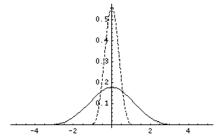
FIG. 1.: $|{{}_{o}\tau}^{+}(x,\tau)|^{2}$ vs. $x$net, with $\Delta=m$ (solid line), and $\Delta=\frac{m}{10}$ (dashed line). As $\Delta$ gets smaller, the probability function gets more and more peaked around the origin.

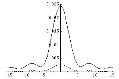
FIG. 2.: $\frac{1}{\epsilon}|{{}_{\epsilon}\tau}^{+}(x,\tau)|^{2}$ vs. $\epsilon x$, with $\Delta\epsilon^{2}=\frac{m}{10}$ (solid line) and $\Delta\epsilon^{2}=\frac{m}{100}$ (dashed line). As $\Delta$ or $\epsilon$ gets smaller, the probability function drops near the origin, and grows longer tails which are exponentially far away.