Non-Markovian quantum trajectories for spectral detection

Abstract

We present a formulation of non-Markovian quantum trajectories for open systems from a measurement theory perspective. In our treatment there are three distinct ways in which non-Markovian behavior can arise; a mode dependent coupling between bath (reservoir) and system, a dispersive bath, and by spectral detection of the output into the bath. In the first two cases the non-Markovian behavior is intrinsic to the interaction, in the third case the non-Markovian behavior arises from the method of detection. We focus in detail on the trajectories which simulate real-time spectral detection of the light emitted from a localized system. In this case, the non-Markovian behavior arises from the uncertainty in the time of emission of particles that are later detected. The results of computer simulations of the spectral detection of the spontaneous emission from a strongly driven two-level atom are presented.

()

Quantum trajectories or stochastic Schrödinger equations [1, 2, 3] have been used as an effective numerical tool (for example [4, 5, 6, 7]) to solve the time evolution of the reduced density matrix for an open system. In addition, a single quantum trajectory simulates the evolution of a system undergoing continuous measurement of its environment [2, 8, 9, 10]. This is of fundamental importance in understanding open system behavior as features of a single realization of a measurement process can be obscured by density matrix methods which average over the individual realizations (see [11] for a dramatic example).

Traditionally, quantum trajectories have described Markov processes, where the conditioned state of the system at a certain time contains all the information needed to calculate the measurement probabilities over the next infinitesimal interval. In this case, a master equation can describe the evolution of the reduced density matrix for the open system. Recently, however, there has been interest in studying open systems for which the Markov approximation cannot be made. For example, in a photonic band-gap material the correlation time of the electromagnetic vacuum fluctuations near a band edge is not small on the timescale of the emitting atomic system [12, 13]. As another example, a Bose-Einstein condensate losing atoms due to a radio-frequency output coupler [14] experiences Non-Markovian decay for certain coupling rates, as the dispersion relation for atoms in free space leads to a non-vanishing correlation time for the atoms coupled out of the condensate [15, 16]. There are also measurement processes that lead to a non-Markovian evolution of the conditioned system [17, 18]. Real-time spectral measurement is an example [19]. In this case, the measurement process yields not only temporal information but also frequency information about the system [20, 21]. It is therefore of interest to generalize quantum trajectory techniques to deal with these non-Markovian processes [23, 24, 25]. In the non-Markovian case the future measurement probabilities need to be calculated from the evolution of the system in the past.

In this paper we formally derive in Sec.I the evolution equation for a non-Markovian trajectory for arbitrary measurement schemes. As an illustrative example we investigate in Sec.II the trajectories that arise from spectral detection of the light from a strongly driven two-level atom.

A derivation of non-Markovian quantum trajectories from a microscopic model (in the case of heterodyne detection [22]) has been made recently by Diòsi and Strutz [24] via path integrals. By rewriting the path integral evolution in terms of operators Diòsi et al. [25] have used this formulation to simulate trajectories for some simple systems with the requirement that the trajectories are consistent with the general formulation. It is not clear (at least to the present authors) what physical situations these trajectories correspond to. In contrast, our formulation is from a measurement theory perspective. We consider a microscopic model and general measurement schemes that are in principle physically realizable. The trajectories are defined from this microscopic model and have an obvious interpretation in terms of the measurements.

A non-Markovian quantum process is one in which the measurement probabilities in the present depend on the evolution of the system in the past. This arises naturally when considering the evolution of an open system conditioned on measurements made on its emission at a distant detector. In a photon counting experiment, for example, the probability of detecting a photon at the detector can, in general, be expressed as the probability for the system to undergo emissions distributed over times in the past. In the Markov case, the probability of a detection is determined by that of a single time of emission. In turn, a measurement result at a particular time does not completely determine the state of the system at the same time. In a Markov process our knowledge of the state of the system straight after the measurement is complete. In the non-Markov case there is a definite evolution that the system must have undergone in the past in order to produce the measurement result, but there is always the possibility that future measurement results will require us to revise our knowledge of the evolution of the system over this same time. However, a conditioned system state can be defined a finite time in the past if we can assume that any events occurring in the system earlier than this time will have a negligible effect on the measurement results in the present.

It is of interest to be able to simulate measurement processes that yield not only temporal information but also frequency information about a system. In other words, real-time spectral measurements, where the emission from the system is passed through a ‘spectrometer’ that splits it into separate spectral components before each component is measured. Real-time spectral measurement is relevant to situations where different spectral components of the emission from a system are time correlated. A well-known example is the three peaked spectrum of the spontaneous emission from a strongly driven two-level atom [26]. In this system the two side peaks are correlated via photon bunching and are individually anti-bunched [20, 27]. The temporal features are not accessible by methods that time average the detections to determine the spectrum. Here we will treat this problem from a real-time spectral detection perspective.

There are two complementary approaches to modeling spectral detection. The first and most physical approach is to model the spectrometer as a separate physical system that is being driven by the output from the system of interest. The whole extended system of system plus spectrometer can then be evolved forward together as a cascaded system [28, 29]. Imamoḡlu [23] has recently developed methods using the extended system approach for the more general case of a mode-dependent coupling to the bath. The second approach, which perhaps coincides more closely with a signal processing treatment, is to consider the spectrometer as a black box where the output from the box is related to the input by a spectral response. Here we will consider the second approach as it is more general and is, we believe, closer to the idea behind quantum trajectories; of simulating a continuous measurement process at a distant detector by evolving a local system forward in time. However, this approach means that we must consider non-Markovian evolution of the system, since emission times become more uncertain as the frequency information becomes more precise.

I Non-Markovian Quantum Trajectories

In this first section we outline the general theory of non-Markovian quantum trajectories from a measurement theory perspective. The form of the system-bath coupling that we consider is given in Sec.I B and we introduce a complete set of measurement channels in Sec.I C to model measurements that are sensitive to only a range of modes of the bath. In Sec.I D we discuss the finite memory-time assumption for the system.

A Measurements on an open system

Consider the typical open system situation of a small localized system surrounded by an infinite bath. The Hamiltonian of the bath and system can be written as the sum of three parts

$$H=H_{\rm sys}+H_{\rm bath}+H_{\rm int},$$ (1)

where $H_{\rm sys}$ is the Hamiltonian of the free system, $H_{\rm bath}$ the Hamiltonian of the free bath and $H_{\rm int}$ the interaction between the two.

An open system can be thought of in terms of inputs and outputs [32]: the initial bath propagates in towards the system; they interact; and the bath propagates away again. We would like to model the situation where measurements are being made continuously on the output bath. The probability of getting a particular string of measurement results ${R}(t,t_{0})$ during the interval $[t,t_{0})$, denoted here by $P[{R}(t,t_{0})]$, is given in terms of the initial state by

$$P[R(t,t_{0})] = {\rm Tr}\left\{|R(t,t_{0})\rangle\langle R(t,t_{0})|\rho(t)\right\},$$ (2)

$$= {\rm Tr}\left\{|R(t,t_{0})\rangle\langle R(t,t_{0})|U_{\rm int}(t,t_{0})\rho(t_{0})U_{\rm int}^{\dagger}(t,t_{0})\right\},$$ (3)

where $U_{\rm int}(t,t_{0})$ is the unitary evolution operator (in the interaction picture) determined by the total Hamiltonian, Eq.(1). Note that we will often use the labels $R$ and $I$ to label both a general element of the set of all possible values and also to represent a particular element of the set. We assume that the system and bath are initially uncorrelated and we can write the initial density matrix in the form $\rho(t_{0})=\rho_{\rm bath}(t_{0})\rho_{\rm sys}(t_{0})$. The density matrix of the bath can be written $\rho_{\rm bath}(t_{0})=\sum_{I}P[I(t,t_{0})]|I(t,t_{0})\rangle\langle I(t,t_{0})|$ where $I(t,t_{0})$ labels a particular pure state of the input bath. Similarly, the system density matrix can be written, $\rho_{\rm sys}(t_{0})=\sum_{k}P[\psi_{k}(t_{0})]|\psi_{k}(t_{0})\rangle\langle\psi_{k}(t_{0})|$. We can now write the probability of the result $R(t,t_{0})$ in the form

$$P[R(t,t_{0})] = \sum_{Ik}P[R(t,t_{0})I(t,t_{0})\psi_{k}(t_{0})],$$ (4)

$$= \sum_{Ik}P[R(t,t_{0})|I(t,t_{0})\psi_{k}(t_{0})]P[I(t,t_{0})]P[\psi_{k}(t_{0})],$$ (5)

where we have used Bayes theorem. From Eq.(3) the conditional probability can be written

$$P[R(t,t_{0})|I(t,t_{0})]=\langle\psi(t_{0})|\Omega^{\dagger}_{RI}(t,t_{0})\Omega_{RI}(t,t_{0})|\psi(t_{0})\rangle,$$ (6)

where we have defined the operation [30] on the system space corresponding to these measurement results over the interval $[t,t_{0})$ as

$$\Omega_{RI}(t,t_{0})=\langle R(t,t_{0})|U_{\rm int}(t,t_{0})|{I}(t,t_{0})\rangle.$$ (7)

Note that we have suppressed the explicit reference to the probability distribution over the initial system states for ease of notation. This is equivalent to assuming that the system was initially in a pure state. The explicit form of the operation $\Omega_{RI}$ for a linear, particle-conserving coupling will be given in Sec.I B. For now, we simply assume that an explicit form exists. The idea behind a quantum trajectory simulation is expressed by Eq.(5). If in a number of runs of the simulation we choose the initial states randomly with a frequency corresponding to the initial probability distribution $P[I(t,t_{0})]$ then the conditional probabilities $P[R(t,t_{0})|I(t,t_{0})]$ of each run will automatically generate values of $R(t,t_{0})$ consistent with $P[R(t,t_{0})]$.

In general, the above operation will not satisfy the semi-group property characteristic of a Markov process, i.e, $\Omega(t,t_{0})\neq\Omega(t,s)\Omega(s,t_{0})$ for all $s$ (we have dropped the subscripts for clarity). However, the operation can always be written in the form

$$\Omega(t,t_{0})=\Omega(t,s)\circ\Omega(s,t_{0}),$$ (8)

where we have defined the $\circ$-product by

$$\Omega(t,s)\circ\Omega(s,t_{0})=\sum_{k}\Omega^{k}(t,s)\Omega^{k}(s,t_{0}).$$ (9)

This is because one can always insert a sum over a complete set of states, $\openone=\sum|k\rangle\langle k|$, at any time in the unitary evolution. The summation in Eq.(9) need not be over the complete set of states, but is over a subset of these that are consistent with both the input and resultant states and therefore depends on the time $s$. The inability to factorize this operation is due to the fact that the system is entangled with the bath at time $s$, so that a measurement of the output at this time does not completely determine the state of the system at the same time.

To understand this we need to consider in more detail the differences between Markovian and non-Markovian evolution of open systems. Firstly, it is not possible to write down a master equation for the reduced system density matrix $\rho_{\rm sys}(t)={\rm Tr}_{\rm bath}\{\rho(t)\}$. This is evident even to first order perturbation in the interaction Hamiltonian during the time interval $T_{\rm m}$,

$$\rho(t)-\rho(t-T_{\rm m})=\int^{t}_{t-T_{\rm m}}ds[H_{\rm int}(s),\rho(t-T_{\rm m})].$$ (10)

where $H_{\rm int}(s)$ is in the interaction picture and we have assumed that the contributions from the state at times before $t-T_{\rm m}$ are negligible. We now write the density matrix at time $t-T_{\rm m}$ in terms of a factorized part and an unfactorized part $\rho(t-T_{\rm m})=\rho^{0}_{\rm sys}(t-T_{\rm m})\rho_{\rm bath}(t_{0})+\chi(t-T_{\rm m})$, where $\chi(t-T_{\rm m})$ contains the entanglement. Inserting this into the above equation and taking the trace over the bath variables we find

$$\rho_{\rm sys}(t)-\rho_{\rm sys}(t-T_{\rm m})={\rm Tr}_{\rm bath}\left\{\int^{t}_{t-T_{\rm m}}ds[H_{\rm int}(s),\chi(t-T_{\rm m})]\right\},$$ (11)

where we have assumed that ${\rm Tr}_{\rm bath}\{H_{\rm int}(s)\rho_{\rm bath}(t_{0})\}=0$, as the mean bath interaction energy can always be taken inside the Hamiltonian for the system. This demonstrates that (even to first order in the perturbation) the change in the density matrix of the system at time $t$ is determined by the correlations that existed between the bath and the system at $t-T_{\rm m}$. Note that the master equation for the system for a Markov process is derived by going to second-order in the perturbation (correlations can only arise from an initial factorized density matrix by going to at least second order in the perturbation) and assuming that the correlations decay instantaneously $T_{\rm m}\rightarrow 0$ on the time scale of the inverse coupling strength (see for example [31]).

Another consequence of the above mentioned entanglement is that to determine the probabilities for a particular measurement result at time $t$ we need to consider the evolution of the system from a time $t-T_{\rm m}$ in the past up until time $t$. In addition, even if the initial state of the system is pure it will not stay pure under evolution conditioned on continuous measurement of the output, unlike the Markov case [2, 9].

Consider the simplest case of continuously counting the emitted particles (e.g., a photodetector counting photons). Suppose that a particle that is detected at time $t$ could only have been emitted during the time interval $[t,t-T_{\rm m})$, with a specific weighting for each possible emission time. Therefore, to determine the probability of a detection at time $t$ we need to propagate the system undergoing emissions over the time interval $[t,t-T_{\rm m})$. A diagram of this situation is given in Fig.1, showing a possible weighting distribution for each emission time for a particle detected at time $t$. Now assume that we have a measurement record over the interval $[t,t-T_{\rm m})$ where a single particle was detected at time $t>t_{1}>t-T_{\rm m}$, (see Fig.1). We have the complete measurement record from $t$ to $t-T_{\rm m}$. Therefore, the conditioned state of the emitting system at time $t-T_{\rm m}$ cannot change due to future detections. We are interested, then, in the conditioned state at time $t-T_{\rm m}$. The detection at time $t_{1}$ corresponds to two possibilities at time $t-T_{\rm m}$, either the particle was emitted after time $t-T_{\rm m}$ or before. In the Hilbert space of the system and bath this corresponds to a superposition of the two possibilities: a particle has been as emitted and is present in the bath and a particle has not been emitted and the bath is empty. In terms of the system alone, when a trace over the bath is performed, this is a mixed state. Note that the mixed state is produced by ignoring the state of the bath. As far as future evolution of the system is concerned there is no classical uncertainty in the state of the system at this time, each of the ket vectors in the density matrix undergo a separate conditioned evolution, determined by the fact that the system must undergo one and only one emission during the interval $[t_{1},t_{1}-T_{\rm m})$ (and also by any future measurement results).

It is a surprising fact that despite these complications it is still possible to derive quantum trajectories for non-Markovian processes.

In order to deal with this sort of mixed conditioned state we generalize the notation of Eq.(9) and write

$$\Omega_{RI}(t,s)\circ|\tilde{\psi}(s)\rangle\equiv\sum_{k}\Omega_{RI}^{k}(t,s)|\tilde{\psi^{k}}(s)\rangle,$$ (12)

where

$$\Omega_{RI}^{k}(s) = \langle R(t,t_{0})|U_{\rm int}(t,s)|k\rangle,$$ (13)

$$|\tilde{\psi^{k}}(s)\rangle = \langle k|U_{\rm int}(s,t_{0})|I(t,t_{0})\rangle|\psi(t_{0})\rangle.$$ (14)

and the tilde denotes that the ket in unnormalized. Note that for any time $s$ there is always one state of the bath, $|I(t,s)\rangle$, that is independent of the measurement results. Let us then take this state as one of the basis states of the bath, $|k=0\rangle\equiv|I(t,s)\rangle$.

Having an explicit form for $\Omega$ means that we are able to calculate the probabilities for the results of measurements made on the output in terms of the conditioned system evolution alone. We will now relate this to simulating the evolution of the measurement process forward in time. To do this in any practical way a necessary requirement is that there exists a time interval $T_{\rm m}$ such that a measurement made at time $t$ will be independent of the state of the system before time $t-T_{\rm m}$. In other words, there must exist a finite memory-time for the open system. We will discuss this in more detail in Sec.I D.

Consider a single run in which we have one particular input state and a record of the results of the measurements during the interval $[t,t_{0})$ and we would like to know the probability of a particular outcome during the next infinitesimal interval. The conditional probability density of getting a particular result during the next infinitesimal interval $[t+dt,t)$ given the previous results over the interval $[t,t_{0})$ is

$$P[R(t+dt,t)|R(t,t_{0})I(t,t_{0})] = \sum_{I(t+dt)}\frac{P[R(t+dt,t_{0})I(t+dt,t_{0})]}{P[R(t,t_{0})I(t,t_{0})]},$$ (15)

$$= \sum_{I(t+dt)}\frac{P[R(t+dt,t_{0})|I(t+dt,t_{0})]}{P[R(t,t_{0})|I(t,t_{0})]}P[I(t+dt,t_{0})|I(t,t_{0})].$$ (16)

If in a simulation we choose the input states consistent with $P[I(t+dt,t)|I(t,t_{0})]$ for each run then $P[R(t+dt,t_{0})|I(t+dt,t_{0})]/P[R(t,t_{0})|I(t,t_{0})]$ will generate results $R(t+dt,t)$ with the required probability distribution. These conditional probability densities can be written in terms of the operation as

$$\frac{P[R(t+dt,t_{0})|I(t+dt,t_{0})]}{P[R(t,t_{0})|I(t,t_{0})]}=\langle\tilde{\psi^{0}}(t+dt)|\tilde{\psi^{0}}(t+dt)\rangle,$$ (17)

where we have defined the system state vector $|\tilde{\psi^{0}}(t+dt)\rangle$, at time $t+dt$, as

$$|\tilde{\psi^{0}}(t+dt)\rangle=|\psi^{0}(t)\rangle+{\mathcal{N}}d\Omega_{RI}(t,t-T_{\rm m})\circ|\psi(t-T_{\rm m})\rangle,$$ (18)

where $|\tilde{\psi^{0}}(t)\rangle=\Omega_{RI}(t,t-T_{\rm m})\circ|\psi(t-T_{\rm m})\rangle$ and ${\mathcal{N}}=1/\sqrt{\langle\tilde{\psi^{0}}(t)|\tilde{\psi^{0}}(t)\rangle}$, again the tilde denotes that the state is unnormalized. This state determines the probabilities for the next measurement results. It is a transient state, in that it can be overwritten by the operation corresponding to subsequent measurement results (it is only the state of the system at time $t$ if the measurement results from $t$ to $t+T_{\rm m}$ correspond to a state equivalent to the input state during this time). In Eq.(18) we have explicitly used the idea that the probabilities of getting a particular measurement result at time $t$ do not depend on the state of the system or bath before time $t-T_{\rm m}$. If this is true then the system state at time $t-T_{\rm m}$ is then $\rho^{RI}_{\rm sys}(t-T_{\rm m})=\sum_{k}P_{k}(t-T_{\rm m})|\psi^{k}(t-T_{\rm m})\rangle\langle\psi^{k}(t-T_{\rm m})|$ and is independent of the measurement results at time $t+dt$. Here, $P_{k}(t-T_{\rm m})={\mathcal{M}}\langle\tilde{\psi^{k}}(t-T_{\rm m})|\tilde{\psi^{k}}(t-T_{\rm m})\rangle$, where ${\mathcal{M}}$ is a constant which ensures that $\sum P_{k}(t-T_{\rm m})=1$. This conditioned state converges to the reduced density matrix for the system when averaged over many runs of the above trajectories, $\rho_{\rm sys}(t-T_{\rm m})=\sum_{IR}\rho^{IR}_{\rm sys}(t-T_{\rm m})$. In the following sections we will investigate the nature of $\Omega$ for a particle conserving coupling and some quite general input states and measurement processes.

B System-bath interaction

We assume that the interaction is linear and conserves particle number and also, for simplicity, that the bath is coupled to a single mode of the system. We consider situations that have bath and interaction Hamiltonians of the form

$$H_{\rm bath} = \int d{\bf k}\omega_{\bf k}b^{\dagger}({\bf k})b({\bf k}),$$ (19)

$$H_{\rm int} = i\sqrt{\gamma}\int d{\bf k}\left\{g_{{\bf k}}b^{\dagger}({\bf k})a-g^{*}_{{\bf k}}b({\bf k})a^{\dagger}\right\},$$ (20)

where we have put $\hbar=1$ and $a$ and $b({\bf k})$ are the annihilation operators for the modes of the system and bath. The bath modes satisfy Bose commutation relations $[b({\bf k}),b^{\dagger}({\bf k^{\prime}})]=\delta({\bf k-k}^{\prime})$. Note that our treatment does not depend on the system being a Bose field. The mode operator could equally well be replaced by, for example, the lowering operator of a two-level atom. The frequency of the ${\bf k}$th mode is $\omega_{\bf k}$ and is an arbitrary function of ${\bf k}$. The effective coupling constant, $g_{{\bf k}}$, is normalized so that $\int d{\bf k}|g_{{\bf k}}|^{2}=1$, and the strength of the coupling is given by $\sqrt{\gamma}$. The spatial dependence of the bath-system coupling determines $g_{{\bf k}}$,

$$\sqrt{\gamma}g_{{\bf k}}=\int d{\bf r}\kappa({\bf r})u^{*}_{\bf k}({\bf r}),$$ (21)

where $\kappa({\bf r})$ is the effective spatially dependent coupling constant and $u_{\bf k}({\bf r})$ are the spatial modes of the bath. An essential assumption in the following derivation is that the system and bath only interact over a finite region $R$ localized about the origin so that we can put $\kappa({\bf r})\approx 0$ for $|{\bf r}|>R$. This is necessary so that we can later make the finite memory-time approximation.

We can define input and output bath fields [15, 32] outside the interaction region ($|{\bf r}|>R$) by

$$b^{\rm in}(t,{\bf r})=\int d{\bf k}b({\bf k},t_{0})e^{-i\omega_{\bf k}(t-t_{0})}u_{\bf k}({\bf r}),$$ (22)

where $t_{0}<t$ can be taken as the initial time and

$$b^{\rm out}(t,{\bf r})=\int d{\bf k}b({\bf k},t_{1})e^{-i\omega_{\bf k}(t-t_{1})}u_{\bf k}({\bf r}),$$ (23)

where $t_{1}>t$ can be taken as a time in the distant future.

The unitary evolution operator $U_{\rm int}(t,t_{0})$ is then given by the total Hamiltonian Eq.(1) in the interaction picture,

$$U_{\rm int}(t,t_{0})=T\exp\left\{i\sqrt{\gamma}\int^{t}_{t_{0}}ds\left[\xi^{\dagger}(s)a_{I}(s)-\xi(s)a_{I}^{\dagger}(s)\right]\right\},$$ (24)

where

$$\xi(t)=\int d{\bf k}g_{{\bf k}}b({\bf k},t_{0})e^{-i\omega_{\bf k}(t-t_{0})},$$ (25)

is the driving field in the Langevin equations of motion for the system mode. $a_{I}(t)$ is the system mode operator in the interaction picture and $T$ denotes that the operators in the exponential are time-ordered. We define a memory function $f_{\rm m}(t-t^{\prime})$ as the commutation relation of the driving field with itself at an earlier time

$$f_{\rm m}(t-t^{\prime}) \equiv [\xi(t),\xi^{\dagger}(t^{\prime})],$$ (26)

$$= \int d{\bf k}|g_{{\bf k}}|^{2}e^{-i\omega_{\bf k}(t-t^{\prime})}.$$ (27)

C Measurement channels

The quantum trajectory formalism presented here is based on an idealized situation where all the output from the bath is eventually measured by a perfectly absorbing measuring device. The physical situations that can be modeled by this formalism are not limited by this, as the information acquired from any measuring device that is not really there in the physical situation can be averaged over a number of runs of the simulated measurement process. So this formalism, although based on measurement theory, contains as a special case even the situation when no measurements are being made at all and the system is simply decaying into the bath.

To describe separate measuring devices it is useful to introduce the concept of a complete set of measurement channels. A measurement channel has an associated field that contains only a range of modes of the original bath field. A measurement made on a particular channel is specific to the particular range of bath modes defined by the channel. The channels form a complete set, in that, together they contain the entire bath field.

In a three-dimensional situation the bath output in all directions is being measured by detectors distributed around the system. To model the situation where each detector is sensitive only to the modes propagating towards it we can define channel fields containing only the appropriate bath modes for each detector. This concept of a channel also stretches to the case of spectral detection, i.e., measurements that directly access spectral information about the output field in a particular direction. A set of measurement channels can be defined such that each channel field contains only a range of frequencies of the output field. In this way, the results of a measurement made on one of these channel fields is specific to the particular range of frequencies defined by the channel.

As a by-product, this formalism allows for the consideration of measurement devices that have a non-trivial spectral response. We can do this by choosing one channel to have the required frequency response, keeping its measurement record, and averaging the measurement results of the other channels (that make up the complete set) over a number of runs.

In summary, we are considering a model where the output from the system passes through a generalized spectrometer, is scattered into different measurement channels and is then measured. The measurements are assumed to take place instantaneously at a single spatial point for each channel. The theory as it stands does not model the situation where the particles can scatter off the measuring device and reinteract with the system.

The generalized linear-passive spectrometer is modeled by splitting the original output bath up into channels. A schematic of the situation is shown in Fig.2. The number of input channels to the spectrometer must equal the number of output channels.

We define the $n$th channel output field by,

$$c^{\rm out}_{n}(t,{\bf r})=\int d{\bf k}S_{n}({\bf k})b({\bf k},t_{1})e^{-i\omega_{\bf k}(t-t_{1})}u_{\bf k}({\bf r})+\mbox{other baths}.$$ (28)

where $S_{n}({\bf k})$ is the spectral response of the channel. The contributions from other free baths (with the same dispersion relation as $b({\bf k})$) do not interact with the system and are initially in a vacuum state. They do not concern us in latter derivations but they are necessary to preserve commutation relations (in other words they have a physical origin).

The definition of the channel fields in Eq.(28) is in fact a linear transform of the mode operators of the independent baths, $b_{m}(k)$, to the mode operators of the channels, $c_{n}(k)$, for each $k$ (we have written ${\bf k}$ as $k$ for ease of notation). Writing $b_{1}(k)=b(k)$ for the original bath modes and defining $c_{n}(k)$ by $c_{n}^{\rm in}(t,r)=\int dkc_{n}(k)e^{-i\omega_{k}(t-t_{0})}u_{k}(r)$, we can write the transformation as

$$c_{n}(k)=S_{n1}(k)b_{1}(k)+\sum_{m\neq 1}S_{nm}(k)b_{m}(k).$$ (29)

The requirement that the channel fields are independent and preserve commutation relations, $[c_{n}(k),c^{\dagger}_{n^{\prime}}(k^{\prime})]=\delta_{nn^{\prime}}\delta(k-k^{\prime})$, is expressed as a constraint on $S_{nm}(k)$,

$$\sum_{m}S_{nm}(k)S^{*}_{mn^{\prime}}(k)=\delta_{nn^{\prime}}$$ (30)

for all $k$. A special case of this when $n=n^{\prime}=1$ is

$$\sum_{m}|S_{m}(k)|^{2}=1.$$ (31)

where we have written $S_{n}(k)=S_{n1}(k)$. This expresses the fact that the channel fields are a complete decomposition of the bath field.

The $n$th output channel field is given by a unitary transform of the $n$th input channel field (the portion of the initial input bath that contributes to the measured output),

$$c_{n}^{\rm out}(t,{\bf r}) = U^{\dagger}_{\rm int}(t,t_{0})c^{\rm in}_{n}(t,{\bf r})U_{\rm int}(t,t_{0}),$$ (32)

$$= \sqrt{\gamma}\int^{t}_{t_{0}}dsh_{n}(t-s,{\bf r})a(s)+c^{\rm in}_{n}(t,{\bf r}).$$ (33)

Note that the channel output fields contain a contribution from the system and the input channel fields.

We have defined $c^{\rm in}_{n}(t,{\bf r})$ as,

$$c^{\rm in}_{n}(t,{\bf r})=\int d{\bf k}S_{n}({\bf k})b({\bf k},t_{0})e^{-i\omega_{\bf k}(t-t_{1})}u_{\bf k}({\bf r})+\mbox{other baths}$$ (34)

and have also defined the impulse response functions, $h_{n}(t-s,{\bf r})$, for each channel, as the commutation relation of $c^{\rm in}_{n}(t,{\bf r})$ with the driving field $\xi^{\dagger}(s)$ at an earlier time,

$$h_{n}(t-t^{\prime},{\bf r}) \equiv [c^{\rm in}_{n}(t,{\bf r}),\xi^{\dagger}(t^{\prime})],$$ (35)

$$= \int d{\bf k}S_{n}({\bf k})g_{\bf k}e^{-i\omega_{\bf k}(t-t^{\prime})}u_{\bf k}({\bf r})$$ (36)

where $t\geq t^{\prime}$. As the $n$th channel field is always measured at the same point in space, ${\bf r}_{n}$, we introduce the notation $h_{n}(t-s)\equiv h_{n}(t-s,{\bf r}_{n})$. Definition Eq.(28) yields the intuitively obvious relation with the output field (see Fig.2),

$$c_{n}^{\rm out}(t,{\bf r})=\int^{t_{1}}_{t}dsh_{n}(t-s)b^{\rm out}(s,{\bf r})+\mbox{other baths}.$$ (37)

The functions $h_{n}(\tau)$ and $f_{\rm m}(\tau)$, defined by the commutation relations Eq.(35) and Eq.(26), completely determine the characteristics of the system-bath interaction and measurement process. In the next subsection we will consider some general properties of these functions.

D Finite memory-time

We now introduce an essential concept, that of the existence of a finite memory-time. That is, we assume that both the memory function and the impulse responses are such that at some finite time in the past $T_{\rm m}$ the following conditions hold

$$\left|\int^{t}_{t-T_{\rm m}}dsf_{\rm m}(t-s)a(s)\right| \gg \left|\int^{t-T_{\rm m}}_{t_{0}}dsf_{\rm m}(t-s)a(s)\right|,$$ (38)

$$\left|\int^{t}_{t-T_{\rm m}}dsh_{n}(t-s)a(s)\right| \gg \left|\int^{t-T_{\rm m}}_{t_{0}}dsh_{n}(t-s)a(s)\right|,$$ (39)

for all $n$ and all $t$ during the entire measurement interval. To guarantee the above condition we assume that the memory and impulse functions satisfy

$$\int^{t}_{t-T_{\rm m}}ds\left|f_{\rm m}(t-s)\right|^{2} \gg \int^{t-T_{\rm m}}_{t_{0}}ds\left|f_{\rm m}(t-s)\right|^{2},$$ (40)

$$\int^{t}_{t-T_{\rm m}}ds\left|h_{n}(t-s)\right|^{2} \gg \int^{t-T_{\rm m}}_{t_{0}}ds\left|h_{n}(t-s)\right|^{2},$$ (41)

which are independent of $a(s)$. These are useful working conditions and are satisfied by all the functions considered in this paper. However, it is also possible to satisfy Eq.(38) and Eq. (39) if the memory function an impulse responses have a rapidly oscillating behavior. In this case the contribution to the integral after some time $t-T_{\rm m}$ may average to zero.

To understand the consequences of a finite memory-time we consider the physical effect of the driving field on the system. The Heisenberg equation of motion for $a(t)$ is

$$\frac{da(t)}{dt}\approx-i[H_{\rm sys},a(t)]-\frac{\gamma}{2}\int^{t}_{t-T_{\rm m}}f_{\rm m}(t-s)a(s)+\xi(t),$$ (42)

where we have neglected the smaller part of the integral. Correlations of the driving field with itself at earlier times cause the evolution of the system to be dependent on its past behavior. The existence of a memory-time implies that there is a finite time after which one can neglect the effect of the past state of the system in determining the present evolution.

The physical effect of the system on the output channel field is given by

$$c_{n}^{\rm out}(t,{\bf r})\approx\sqrt{\gamma}\int^{t}_{t-T_{\rm m}}dsh_{n}(t-s,{\bf r})a(s)+c^{\rm in}_{n}(t,{\bf r}),$$ (43)

where we have again explicitly inserted the lower bound of the integral. From this equation one can see that the state of the system in the past determines the output channel field in the present and that the finite memory time imposes a cutoff time for this dependence. This relation highlights an important point regarding the interpretation of the results of measurements of the output channels in terms of the system dynamics. A measurement result at time $t$ does not mean that we can ascribe a state corresponding to this result to the system at the same time $t$. Unmeasured output at later times is still quantum mechanically entangled with the system at time $t$ and a subsequent measurement could require us to revise our knowledge of the system state completely. In the Markov case, because of the delta function impulse response, a measurement result meant that we could specify the state of the system at the same time. In the general case considered here, only states of the system at a time $t-T_{\rm m}$ can be thought of as fully specified, as the output after time $t$ is uncorrelated with the system before this time and future measurements will not alter our knowledge of the system state. We can then interpret the state at time $t-T_{\rm m}$ as the system state conditioned on the measurements up to and including time $t$.

E Conditioned system evolution

We now return to a treatment in terms of state vectors and set about determining the explicit form of $\Omega_{RI}$ for a general measurement scheme.

We consider quantum trajectories to be an attempt to simulate the measurement results of a distant measuring device by the evolution of a local system emitting particles. This is related to the way in which the spectrometer is treated in this work. Instead of explicitly modeling the generalized spectrometer as a physical system (coupled to our localized system) we move towards a signal processing treatment, where the spectrometer is treated as a black box and its inputs are related to its outputs via a spectral response.

Take, for example, a number of measuring devices making particle counting measurements. At any one time we assume that there are only two possible outcomes (for perfect detectors): the null result, where no particle is present at any of the detectors; and the positive result, where a particle is detected at a single detector. A positive result corresponds, in general, to a superposition of particle emissions from the system at times in the past. Therefore, a probability can be calculated for the event from only the evolution of the system undergoing emissions. We assume that the weighting given to each emission time characterizes completely the passage of the particle to the detectors. The probability of the null event can be inferred from the requirement that the probabilities of all possible measurement results must add up to one. The probability of the null event cannot be determined directly as we are not explicitly modeling the physical evolution of the particle from the system to the detector.

It is a rather interesting fact that in the spectral detection case the null result, the no detection result, cannot be assigned an operation. In the Markovian quantum trajectory case a null result corresponds precisely to a non-emission event (a virtual emission and absorption) and so an operation is also assigned to the null event. The virtual emission-absorption event is localized in the interaction region and so is not directly related to results at the distant detector. However, in the Markovian case the detector can in principle be brought right up against the interaction region (which takes place at a point in the Markovian case).

Recall that we have defined the operation in the system space corresponding to the measurement results over the interval $[t,t_{0})$ as

$$\Omega_{RI}(t,t_{0})=\langle{R}(t,t_{0})|U_{\rm int}(t,t_{0})|{I}(t,t_{0})\rangle,$$ (44)

where $U_{\rm int}(t,t_{0})$ is given by Eq.(24). We are trying to simulate the measurement process in terms of the evolution of the system alone and so have not included the spectrometer in the unitary evolution. The operation contains all the information about how to evolve the system forward conditioned on measurement results and also how to calculate the probability of a particular outcome.

We assume that our idealized measuring devices yield a result for each infinitesimal interval of the continuous measurement process. The state corresponding to the results must then factorize into a product of states over each infinitesimal interval. We can therefore write the output state as a product of state generators over each infinitesimal interval acting on the vacuum. We consider measurements where the generator for the output is written as a function of the creation operators for the free input channel fields at a particular position $c_{n}^{\dagger{\rm in}}(t,{\bf r}_{n})$, (the measurement apparatus can be thought of as a sink for particles at position ${\bf r}_{n}$). In mathematical language we have,

$$|{R}(t,t_{0})\rangle=\prod_{n,j}G^{R}_{j,n}[c^{\dagger{\rm in}}_{n}(t_{j},{\bf r}_{n})]|\{0\}\rangle,$$ (45)

where $G^{R}_{j,n}[c_{n}^{\dagger{\rm in}}(t_{j},{\bf r}_{n})]$ is the generator of the state during the interval $[t_{j}+dt,t_{j})$ where $t_{j}$ ranges from $t_{0}$ to $t-dt$. The input channel operator appears in this expression because it is the interaction picture output channel field. For example, these generators may correspond to measurements of the quadrature amplitudes (homodyne [2] and heterodyne detection [22]) or absorption measurements (particle counting)[2].

The input can similarly be thought of as a source of particles at positions ${\bf q}$ and is written in terms of the input field, i.e.,

$$|{I}(t,t_{0})\rangle=\prod_{j}G^{I}_{j}[b^{\dagger{\rm in}}(t_{j},{\bf q})]|\{0\}\rangle.$$ (46)

For example, these generators can correspond to vacuum or coherent input states, squeezed input states or thermal input states [1, 4].

Recall that our problem is to determine the operation $\Omega_{RI}(t,t_{0})$ in terms of the system variables only. Because of the factorized form of the input and output state we can consider operations of the form

$$O_{n}(t_{j})=\langle\{0\}|G_{j,n}^{R}[c_{n}^{\rm in}(t_{j},{\bf r}_{n})]U_{\rm int}(t,t_{0})G_{j}^{I}[b^{\dagger{\rm in}}(t_{j},{\bf q})]|\{0\}\rangle,$$ (47)

for each $t_{j}$ and each channel $n$.

To proceed further we note that we can write the interaction unitary evolution operator $U_{\rm int}(t,t_{0})$ in the form

$$U_{\rm int}(t,t_{0})=T_{a}\left\{V_{+}V_{0}V_{-}\right\},$$ (48)

where $T_{a}$ denotes time-ordering of the system operators $a_{I}$ and $a_{I}^{\dagger}$ and where

$$V_{+} = \exp\left\{\sqrt{\gamma}\int^{t}_{t_{0}}ds\xi^{\dagger}(s)a_{I}(s)\right\},$$ (49)

$$V_{0} = \exp\left\{-\frac{\gamma}{2}\int^{t}_{t_{0}}ds_{2}\int^{s_{2}}_{t_{0}}ds_{1}f_{\rm m}(s_{2}-s_{1})a_{I}^{\dagger}(s_{2})a_{I}(s_{1})\right\},$$ (50)

$$V_{-} = \exp\left\{-\sqrt{\gamma}\int^{t}_{t_{0}}ds\xi(s)a^{\dagger}_{I}(s)\right\}.$$ (51)

This can be proved by differentiating $U_{\rm int}(t,t_{0})$ and re-ordering the bath operators. The operation $O_{n}(t_{j})$ then becomes

$$O_{n}(t_{j})=\langle\{0\}|T_{a}\left\{G^{R}_{j,n}[c^{\rm in}_{n}(t_{j},{\bf r}_{n})]V_{+}V_{0}V_{-}G_{j}^{I}[b^{\dagger{\rm in}}(t_{j},{\bf q})]\right\}|\{0\}\rangle,$$ (52)

where we have expanded the brackets of the time-ordering to encompass the state generators as they are only a function of the bath operators.

We now make use of the relation (compare with Eq.(28))

$$V_{-}b^{\dagger{\rm in}}(t,{\bf q})V_{-}^{-1} = b^{\dagger{\rm in}}(t,{\bf q})+\sqrt{\gamma}{\mathcal{A}}^{\dagger}(t,t_{0};s),$$ (53)

$$V_{+}^{-1}c^{\rm in}_{n}(t,{\bf r}_{n})V_{+} = c^{\rm in}_{n}(t,{\bf r}_{n})+\sqrt{\gamma}{\mathcal{A}}_{n}(t,t_{0};s)$$ (54)

where we have defined for notational purposes

$${\mathcal{A}}_{n}(t,t_{0};s) \equiv \int^{t}_{t_{0}}dsh_{n}(t-s)a_{I}(s),$$ (55)

$${\mathcal{A}}(t,t_{0};s) \equiv \int^{t}_{t_{0}}ds[b^{\rm in}(t,{\bf q}),\xi^{\dagger}(s)]a_{I}(s).$$ (56)

We then make the above replacements and note that $V_{-}$ can be annihilated on the right-hand vacuum and $V_{+}$ on the left-hand vacuum. The the system operators $a_{I}$ and $a_{I}^{\dagger}$ commute with all the input fields $c^{\rm in}_{n}(t_{j},{\bf r}_{n})$ and $b^{\rm in}(t_{j},{\bf q})$, as they are still inside the time-ordering brackets and so act like complex numbers.

If we repeat this procedure for each time $t_{j}$ and if we restrict the nature of the state generators so that when the $R$ and $I$ generators for each time are swapped from left to right no bath modes are left that are not normally-ordered (specific examples will be given latter) then we are left with an operation of the form

$$\Omega_{RI}(t,t_{0})=T\left\{\prod_{j,n}G_{j,n}^{R}[\sqrt{\gamma}{\mathcal{A}}_{n}(t_{j},t_{0};s)]V_{0}\prod_{j}G^{I}_{j}[\sqrt{\gamma}{\mathcal{A}}^{\dagger}(t_{j},t_{0};s)]\right\},$$ (57)

where we have dropped the reference to the mode operators in the time ordering operator $T$.

This is the general result for arbitrary (with the above restriction) measurement schemes and arbitrary input. No assumptions have been made regarding the strength of the coupling constant or the nature of the correlations between the system and the bath after the initial time. This operation can be transformed to the Schrödinger picture by multiplying on the left by the unitary evolution operator for the free system.

Because of the complex nature of the above operation the measurement process can only be simulated on a computer in the weak-interaction short-memory-time case where $I(t)/\Gamma<1$, for all times of interest, where $I(t)=\langle b^{\dagger{\rm out}}(t)b^{\rm out}(t)\rangle\sim\gamma\langle a^{\dagger}(t)a(t)\rangle$ is the intensity of the output. $\Gamma\sim 1/T_{\rm m}$ is some measure of the rate of decay of the of the memory function or impulse response. It determines, in essence, how non-Markovian the process is. In this situation we can make a perturbative expansion of the operation $\Omega_{RI}$ in powers of $\gamma\langle a^{\dagger}(t)a(t)\rangle/\Gamma$. To lowest orders the dimensionality of the integrals during a memory-time will be small and they can be evaluated numerically with a computer. In absorption measurements each click of the counter corresponds to one integral so this can be simulated in the case where there are on average only a few detections (real emissions) during a memory-time (there will also be integrals of the same dimension corresponding to virtual emission-absorption events). We shall explicitly demonstrate how this can be done in the case of optical spectral detection in the next section.

II Optical spectral detection

In this section we consider a special case of the above theory; that of spectral detection of an optical field emitted from a source. To check the accuracy of our numerical simulations we shall apply it to a known problem; the spectral measurement of light emitted from a strongly driven two-level atom.

Spectral detection of an optical field is defined here as meaning that each photodetection can be identified with the emission of a photon from a certain part of the source spectrum [19] (this is in contrast to measurements from which the spectrum can be computed, such as heterodyne detection). Spectral detection necessarily involves the interference of light emerging from the system over some time period $\Delta t$. The length of this time period varies inversely with the accuracy of the spectral measurement.

The type of spectral detection that has been considered previous to this work is that of detecting fields with spectral peaks of widely differing frequencies. These are then just treated as independent Markovian baths for the source to decay into. The evolution of the wave function for this type of system can then be treated with the standard quantum trajectory approach. Here we would like to go beyond this and treat wave function evolution for the source conditioned on spectral detection of emitted photons within an emission linewidth. To achieve this it is necessary to give up knowledge of the exact time of emission. We can only know the time of emission to within an interval $\Delta t>1/\Delta\omega$ if we are to resolve the emission spectrum to within $\Delta\omega$ of a certain frequency.

A The spectrum of a strongly driven two level atom

A strongly driven two-level atom can be described (in a frame rotating at the frequency of the driving field) by the free system Hamiltonian,

$$H_{\rm atom}=\frac{\Omega}{2}(\sigma^{\dagger}+\sigma),$$ (58)

where $\sigma$ is the lowering operator and $\Omega$ is the classical driving field strength and we have assumed that the driving field is on resonance with the atomic transition.

The optical field interacts with the atom in a very small region about ${\bf r}=0$ and we can write the unitary evolution Eq.(24) as

$$U_{\rm int}(t,t_{0})=T\exp\left\{i\sqrt{\gamma}\int^{t}_{t_{0}}ds\left[\sigma^{\dagger}_{I}(s)\xi(s)-\sigma_{I}(s)\xi(s)\right]\right\},$$ (59)

where in this case

$$\xi(t)=\int^{\infty}_{-\infty}d\omega b(\omega,t_{0})e^{-i\omega(t-t_{0})}.$$ (60)

We have replaced the mode label ${\bf k}$ by the angular frequency $\omega$ as is customary in optics in the situation when the direction of the emitted light is unimportant. We have also ignored the polarization of the light field. Note that $\xi(t)$ is the same as the free input field at the point of interaction ${\bf r}=0$ and it is delta-correlated with itself, $[\xi(t),\xi^{\dagger}(t^{\prime})]=\delta(t-t^{\prime})$. Because of this delta function correlation of the driving field a Markovian master equation can be derived for the system by tracing over the bath (see [31] for example). Here we will consider a non-Markovian unraveling [2] of this master equation into quantum trajectories .

It has been shown by Mollow [26] that the spectrum of the spontaneous emission from a strongly driven two-level atom has three peaks at the frequencies $0$, $\pm\Omega$. It has also been shown by Cohen-Tannoudji and Reynaud [20] that the side-bands exhibit photon antibunching independently, but are correlated via photon bunching. Experiments by Aspect et al. [27] have confirmed these theoretical results by frequency filtering the light incident on three photodetectors, so that each photodetector is only sensitive to a range of frequencies about one of the peaks of the output light. Here we would like to reproduce these well known results by simulating this “spectral detection” of the spontaneously emitted light with a non-Markovian quantum trajectory for the source atom.

The original theoretical predictions were made with a fully quantized atom-field model and the model was analyzed in terms of the eigenstates of the Hamiltonian, the dressed states of the atom. Instead, we will consider the simplified model described by the Hamiltonian above, Eq.(58). In the limit of a large classical driving the field can be assumed to be in a coherent state and our model is valid. All the important results of the dressed state model will be present in our treatment [19]. We can qualitatively understand the behavior of this system by considering the evolution of the interaction-picture lowering operator,

$$\sigma_{I}(t)=\textstyle{\frac{1}{2}}\left(\sigma_{x}+|+\rangle\langle-|e^{i\Omega t}+|-\rangle\langle+|e^{-i\Omega t}\right)$$ (61)

where $|+\rangle,|-\rangle$ are the eigenstates of $\sigma_{x}=\sigma_{+}+\sigma_{-}$, $\sigma_{x}|\pm\rangle=\pm|\pm\rangle$. If we are continuously monitoring the emission from the system and are able to resolve the frequencies of the emitted photons, then if a photon is detected in the $+\Omega(-\Omega)$ frequency peak the system will be projected into the opposite eigenstate $|-\rangle(|+\rangle)$. If, however, a photon is detected in the central or zero frequency peak the value of $\langle\sigma_{x}(t)\rangle$ will be unchanged. The interesting behavior of this system stems from this simple idea.

In the following sections we will only consider the case of direct detection, that is, absorption measurements by photodetection. The state corresponding to an absorption measurement in one of the spectral channels during an infinitesimal interval is

$$|{R}(t+dt,t)]\rangle=\prod_{n}c_{n}^{\dagger{\rm in}}(t)^{dN_{n}(t)}|\{0\}\rangle,$$ (62)

where the restrictions $(\sum_{n}dN_{n}(t))^{2}=\sum_{n}dN_{n}(t)$ and $dN_{n}(t)^{2}=dN_{n}(t)$ describe a point process, such that in an infinitesimal interval, either only one photon is detected in one of the channels or no photons are detected in any of the channels. The $dN_{n}(t)$ can take the value $1$ or $0$ corresponding to a click of the photodetector for channel $n$ and no click of the photodetector. We also assume that the input state is the vacuum (the coherent driving being included in the system Hamiltonian).

Consider the situation where $N$ photons have been detected at each of the times $t_{1}<t_{2}<\cdots<t_{i}<\cdots<t_{N}$ in the channels $n_{1},n_{2},\ldots,n_{i},\ldots,n_{N}$ during the past interval $[t,t-T_{\rm m})$. The wavefunction Eq.(18)for the next infinitesimal interval is

$$|\tilde{\psi^{0}}(t+dt)\rangle = |\psi^{0}(t)\rangle-dt\frac{\gamma}{2}\sigma_{I}^{\dagger}(t)\sigma_{I}(t)|\psi^{0}(t)\rangle$$ (63)

$$+ \sum_{n}dN_{n}(t)\left[{\mathcal{N}}\sqrt{\gamma}\sum^{2^{N}}_{i=1}\int^{t}_{t-T_{\rm m}}dsh_{n}(t-s)T\left\{\sigma_{I}(s)\Lambda^{i}(t,t-T_{\rm m})\right\}|\psi^{i}(t-T_{\rm m})\rangle-|\psi^{0}(t)\rangle\right],$$ (64)

where

$$\Lambda^{i}(t,t-T_{\rm m})=\prod\sqrt{\gamma}{\mathcal{A}}_{n_{j}}(t_{j},t-T_{\rm m};s_{j})V_{0}(t,t-T_{\rm m}),$$ (65)

and

$${\mathcal{A}}_{n_{j}}(t_{j},t-T_{\rm m};s)\equiv\int^{t_{j}}_{t-T_{\rm m}}dsh_{n_{j}}(t_{j}-s)\sigma_{I}(s).$$ (66)

In this case $V_{0}(t,t-T_{\rm m})=\exp\{-\frac{\gamma}{2}\int^{t}_{t-T_{\rm m}}dsa_{I}^{\dagger}(s)a_{I}(s)\}$, this leads to a much simpler evolution than the general case. The integrals ${\mathcal{A}}_{n_{j}}(t_{j},t-T_{\rm m};s)$ have the lower bound $t-T_{\rm m}$. However, there is no factorization of the operation at $t-T_{\rm m}$. Instead, we must write a different state vector for each $\Lambda^{i}$. The product is over each combination of from $0$ to $N$ integrals. To understand what we have done here it is necessary to look at the integrals more carefully. Consider, as an example, two time-ordered integrals,

$$T\{{\mathcal{A}}_{n_{1}}(t_{1},t_{1}-T_{\rm m},s_{1}){\mathcal{A}}_{n_{2}}(t_{2},t_{2}-T_{\rm m},s_{2})V^{0}(t,t_{2}-T_{\rm m})\}=\int^{t_{1}}_{t_{1}-T_{\rm m}}\int^{t_{2}}_{t_{2}-T_{\rm m}}T\left\{\cdots\right\},$$ (67)

where $t>t_{1},t_{2}>t-T_{\rm m}$. For each detection at time $t_{i}$ there is an integration over emission times during the interval $[t_{i},t_{i}-T_{\rm m})$. If we split both integrals into the sum of two parts - emissions before $t-T_{\rm m}$ and emissions after - we can write this as the sum of four terms

$$\int^{t_{1}}_{t_{1}-T_{\rm m}}\int^{t_{2}}_{t_{2}-T_{\rm m}}T\left\{\cdots\right\} = \int^{t_{1}}_{t-T_{\rm m}}\int^{t_{2}}_{t-T_{\rm m}}T\left\{\cdots\right\}T\left\{\cdots\right\}+\int^{t_{1}}_{t-T_{\rm m}}T\left\{\cdots\right\}\int^{t-T_{\rm m}}_{t_{2}-T_{\rm m}}T\left\{\cdots\right\}$$ (68)

$$+ \int^{t_{2}}_{t-T_{\rm m}}T\left\{\cdots\right\}\int^{t-T_{\rm m}}_{t_{1}-T_{\rm m}}T\left\{\cdots\right\}+T\left\{\cdots\right\}\int^{t-T_{\rm m}}_{t_{1}-T_{\rm m}}\int^{t-T_{\rm m}}_{t_{2}-T_{\rm m}}T\left\{\cdots\right\}.$$ (69)

This can be easily generalized to $N$ integrals. This is the essence of what has been done in Eq.(64). The parts of the integrals before $t-T_{\rm m}$ get absorbed into wave functions. Each wavefunction is labeled so that its subsequent evolution is consistent with its previous evolution. Physically this means that if a photon is detected in a channel at a particular time this corresponds to a sum over individual emission events and a photon cannot be emitted more than once. This is the detailed structure glossed over in the $\circ$-product notation of the previous section.

The probability density for a detection to occur in channel $n$ during the time interval $[t+dt,t)$ conditioned on the previous detections is then given by

$$P_{n}(t+dt|t_{N},t_{N-1},\cdots,t_{1})=\langle\tilde{\psi_{n}^{0}}(t+dt)|\tilde{\psi_{n}^{0}}(t+dt)\rangle,$$ (70)

where

$$|\tilde{\psi_{n}^{0}}(t+dt)\rangle={\mathcal{N}}\sqrt{\gamma}\sum^{2^{N}}_{i=1}\int^{t}_{t-T_{\rm m}}dsh_{n}(t-s)T\left\{a_{I}(s)\Lambda^{i}(t_{i},t_{i}-T_{\rm m})\right\}|\psi^{i}(t-T_{\rm m})\rangle.$$ (71)

This result is of limited practical use in the above form as evaluating multi-dimensional integrals on a computer is a slow business. Instead we take a less ambitious approach and assume that the bath-system coupling is weak so that we can make what amounts to a perturbative expansion of the trajectory in terms of the coupling strength $\sqrt{\gamma}$. In other words, we assume that on average only a small number of detections occur during the time interval $[t,t-T_{\rm m})$, the number of detections determining the dimension of the integration. To first order, i.e., when the maximum number of detections per memory time is one, the trajectory is very similar to the Markovian case. We therefore consider the next highest order so that there is a finite possibility of two detections occurring per memory time.

In order to demonstrate how a trajectory is simulated on a computer in practice, we write down as an example the Schrödinger picture form of Eq.(71) in the case where one detection occurred at time $t^{\prime}$ in channel $n^{\prime}$ during the previous memory time,

$$\frac{|\tilde{\psi^{0}_{n}}(t+dt)\rangle}{\mathcal{N}}=\gamma\int^{t}_{t^{\prime}}\!ds_{1}\int^{t^{\prime}}_{t-T_{\rm m}}\!\!\!ds_{2}h_{n}(t-s_{1})h_{n^{\prime}}(t^{\prime}-s_{2})U_{\rm eff}(t,s_{1})\sigma U_{\rm eff}(s_{1},s_{2})\sigma U_{\rm eff}(s_{2},t-T_{\rm m})|\psi^{0}(t-T_{\rm m})\rangle$$ (74)

$$+\gamma U_{\rm eff}(t,t^{\prime})\int^{t^{\prime}}_{t-T_{\rm m}}\!\!\!ds_{1}\int^{s_{1}}_{t-T_{\rm m}}\!\!\!ds_{2}[h_{n}(t-s_{1})h_{n^{\prime}}(t^{\prime}-s_{2})]_{\rm sym}U_{\rm eff}(t^{\prime},s_{1})\sigma U_{\rm eff}(s_{1},s_{2})\sigma U_{\rm eff}(s_{2},t-T_{\rm m})|\psi^{0}(t-T_{\rm m})\rangle$$

$$+\sqrt{\gamma}\int^{t}_{t-T_{\rm m}}\!\!\!dsh_{n}(t-s)U_{\rm eff}(t,s)\sigma U_{\rm eff}(s,t-T_{\rm m})|\psi^{1}(t-T_{\rm m})\rangle.$$

where $U_{\rm eff}(t,t_{0})=\exp\{[-iH_{\rm atom}-\frac{\gamma}{2}\sigma^{\dagger}\sigma](t-t_{0})\}$ and $[h_{n}(t-s_{1})h_{n^{\prime}}(t^{\prime}-s_{2})]_{\rm sym}=h_{n}(t-s_{1})h_{n^{\prime}}(t^{\prime}-s_{2})+h_{n}(t-s_{2})h_{n^{\prime}}(t^{\prime}-s_{1})$. The right-hand side is the sum of three terms. The first term represents the situation where the emission corresponding to the detection at $t^{\prime}$ occurs after time $t-T_{\rm m}$ but before the emission that is detected at time $t$. The second term represents the situation where both the $t$ emission and the $t^{\prime}$ emission occur during the same time interval $[t^{\prime},t-T_{\rm m})$ and the time-ordering of the emission is accounted for by the symmetric ordering of the impulse response functions. In the last term the time $t^{\prime}$ emission has occurred before time $t-T_{\rm m}$ (and is included in $|\psi^{1}(t-T_{\rm m})\rangle$) and only the time $t$ emission is left. The states $|\psi^{i}(t-T_{\rm m})\rangle$ are propagated forward one time step $dt$ by doing the integrations contained in the operation from $t-T_{\rm m}$ to $t-T_{\rm m}+dt$.

An important technical aspect of the simulation is; how to choose a finite length impulse response for numerical calculations given a particular spectral response? This is a problem of signal analysis and numerical routines exist for automatically generating finite length impulse responses from a given spectral response such that the spectral response corresponding to the finite length impulse response is as close as possible to the original in a least-squares min-max sense [33]. Note that if the impulse response is too long there is a greater chance of having to deal with higher-order integrals, while if it is too short the spectral response will not approximate the original spectral response and the probabilities will not be accurate. In line with this we have avoided triple integrals by shortening the response functions when calculating the probabilities for detection after two detections have already occurred during the previous memory-time. As the probability of three detections during a memory time is already small (in the limit of weak damping) this should not have a large effect on the statistics of the counts.

The simulation procedure at each time step $dt$ is as follows. First, the conditional probabilities for detections at time $t+dt$ in each of the channels during the time step is generated by calculating the wave function Eq.(74) for each $n$. This depends on any previous detections during the time interval. The normalization ${\mathcal{N}}=\langle\tilde{\psi^{0}}(t)|\tilde{\psi^{0}}(t)\rangle$ must also be calculated independently at each time step by propagating from $t-T_{\rm m}$ to $t$ conditioned on previous detections but assuming that there will be no more detections during the time interval $[t+T_{\rm m},t)$. The probabilities for detections in each channel are added together and compared to a random number. If the probability of a count is less than the random number, the state at time $t-T_{\rm m}$, $|\psi^{(i)}(t-T_{\rm m})\rangle$ is propagated forward conditioned on the fact that there was no detection at time $t+dt$. If the probability of a count was greater than the random number a channel is randomly picked from the probability distribution over the channels. The state at time $t-T_{\rm m}$ is then propagated forward $dt$ conditioned on this outcome. The process can then begin again.

1 The Frequency Filter

Here we consider the situation where we frequency filter the output from the atomic source. The light emitted from the source passes through a Faraday isolator (so the filter cannot affect the source) and then through the filter. It is therefore possible, by tracing over both the bath and the filter cavity, to write down a master equation for the source alone.

We consider as a frequency filter a two-sided Fabry-Perot cavity that can reflect and also transmit light. The coupling strength $\kappa$ is assumed to be the same at each mirror. The transmitted light will be in a Lorentzian shaped band of width $\kappa$ about the resonance frequency of the cavity, $\nu$. This light is detected by a photodetector as is the light reflected from the other mirror.

The reason that the non-Markovian quantum trajectory for the evolution of the atom can generate the correct probabilities for the spectral detection without explicitly modeling the filter cavity (with a Hamiltonian) is because it is possible to eliminate the filter cavity mode completely and write the output from the cavity in terms of the input [34].

We define two output channels, $c^{\rm out}_{R}$ and $c^{\rm out}_{T}$, as the two output fields from the reflecting and transmitting mirrors, respectively, after the output from the atom $b^{\rm out}$ has interacted with the filter cavity,

$$c^{\rm out}_{R}(t) = U^{\dagger}_{F}(t,t_{0})[b^{\rm out}(t)+c_{T}^{\rm in}(t)]U_{F}(t,t_{0}),$$ (75)

$$= b^{\rm out}(t)+c_{T}^{\rm in}(t)+\sqrt{\kappa}a(t),$$ (76)

$$c^{\rm out}_{T}(t) = U^{\dagger}_{F}(t,t_{0})[b^{\rm out}(t)+c_{T}^{\rm in}(t)]U_{F}(t,t_{0}),$$ (77)

$$= b^{\rm out}(t)+c_{T}^{\rm in}(t)+\sqrt{\kappa}a(t),$$ (78)

where $U_{F}$ is the unitary evolution for the interaction of the baths with the filter defined by

$$U_{F}(t,t_{0})=T\exp\left\{i\sqrt{\kappa}\int^{t}_{t_{0}}ds\left(a_{I}(s)[c_{T}^{\dagger{\rm in}}(s)+b^{\dagger{\rm out}}(s)]-H.c.\right)\right\},$$ (79)

where $a_{I}(s)$ is the cavity mode in the interaction picture, $c_{T}^{\dagger{\rm in}}(s)$ is the free transmitted field and $b^{\rm out}(s)$ is the output field that is coupled to the atom, both are delta correlated.

We can now easily solve the Heisenberg equations of motion for the filter cavity mode by Fourier transforms. If we assume the state of the filter in the distant future is the vacuum state we can put $a(t_{1})=0$, and we find

$$c^{\rm out}_{R}(t) = \frac{1}{\sqrt{2\pi}}\int^{\infty}_{-\infty}d\omega\frac{i(\omega-\nu)b(\omega,t_{1})+\kappa c_{T}(\omega,t_{1})}{\kappa-i(\omega-\nu)}e^{-i\omega(t-t_{1})},$$ (80)

$$c^{\rm out}_{T}(t) = \frac{1}{\sqrt{2\pi}}\int^{\infty}_{-\infty}d\omega\frac{i(\omega-\nu)c_{T}(\omega,t_{1})+\kappa b(\omega,t_{1})}{\kappa-i(\omega-\nu)}e^{-i\omega(t-t_{1})},$$ (81)

These are the channel field operators corresponding to photodetections of the reflected and transmitted fields of the filter. The presence of the bath $c_{T}$ preserves commutation relations. The impulse response for each of these channels are therefore,

$$h^{\rm filter}_{R}(t-s) = \frac{1}{\sqrt{2\pi}}\int^{\infty}_{-\infty}d\omega\frac{i(\omega-\nu)}{\kappa-i(\omega-\nu)}e^{-i\omega(t-s)},$$ (82)

$$= -\delta(t-s)+h^{\rm filter}_{T}(t-s),$$ (83)

$$h^{\rm filter}_{T}(t-s) = \frac{1}{\sqrt{2\pi}}\int^{\infty}_{-\infty}d\omega\frac{\kappa}{\kappa-i(\omega-\nu)}e^{-i\omega(t-s)},$$ (84)

$$= u(t-s)\kappa e^{-i\nu(t-s)}e^{-\kappa(t-s)},$$ (85)

where $u(\tau)$ is the unit step function, zero for $\tau<0$. Note that in line with the general discussion in the introduction if we detect a photon in the channel $c^{\rm out}_{T}$ then we know its frequency to within the cavity linewidth $\kappa$ but have lost information about the time of emission to within $1/\kappa$.

We can simulate the spectral measurement process via Eq.(64) by simply substituting in the filter impulse responses. The perturbation expansion in this case is in orders of $\gamma/\kappa$ as $\kappa$ defines the decay time of the impulse response functions.

Fig.3 is a schematic of the situation in frequency space, showing the three peaked output and a superimposed cavity filter centered on the central peak. In this situation the central peak is transmitted while the two side peaks are reflected by the filter.

The results of a simulation with the parameters of Fig.3 are shown in Fig.4 where we have plotted the photodetection waiting times for the reflected and transmitted emission for one run of a total of $12\times 10^{4}$ detections. The time average of a single realization is equivalent to an ensemble average. The transmitted light is mostly from the central peak and the reflected from the side peaks. Notice that both these waiting-time distributions show a marked increase in the frequency of longer waiting times compared to the distribution for the combined emission. As $\gamma\sim\kappa$ the resolution of the spectral detection was of the order of the decay linewidth. This is reflected in the fact that a non-vanishing fraction of the photons were detected within a memory time $T_{\rm m}=1/\gamma$ of each other.

A plot of the evolution of the probabilities of the two channels for the first ten detections of a single trajectory is shown in Fig.5. The probability of a transmission is proportional to the expectation value of the number of photons in the filter cavity. When there are no detections it oscillates at the frequency $\Omega$, in time with the oscillation of $\langle\sigma_{y}(t)\rangle$. The probability of detecting a reflected photon is an interference between the possibility of a photon being reflected directly off the mirror and the possibility of a photon coming back out of the cavity through the reflecting mirror. The oscillations are suppressed by this interference. The possibility of detecting a reflected photon is very sensitive to the phase between the states representing these two possibilities, an example is the large peaks in the reflected probability when a photon is detected in the reflected channel and the oscillation has the right phase.

Fig.6 is a plot of the time evolution of the conditioned evolution of the expectation value of $\sigma_{x}$ and $\sigma_{y}$ during the same trajectory. Note that the conditioned system shows signs of having started to emit even before a detection occurs. This is clearest in the decaying $\langle\sigma_{y}(t)\rangle$ oscillation before the second and sixth detection. This is a clear indication of the non-Markovian behavior of the conditioned state; measurement probabilities depend on the previous state of the system and the conditioned state of the system is affected by a detection at a later time. The interpretation of this behavior goes as follows: at the time of detection the system + bath is in a superposition of all the possible states, a detection selects out the state that corresponds to one particle in the bath; associated with this state is a particular history, i.e., a weighted sum of emission times; this history then determines the conditioned state. In the filter cavity case $\sigma_{x}$ is a constant of the free motion and is unaffected by the measurement process as the measurement does not distinguish between the sidebands.

This situation can also be written in terms of the theory of cascaded systems [28, 29]. In that case, the evolution of the filter cavity as well as the atomic system are treated together as a coupled system. This is a special case of the more general idea that was mentioned in the introduction. The atom and the filter are coupled to the reflected bath at the same physical location and they are also coupled together directly. The quantum trajectory is then evolved by simulating the conditioned evolution of the complete system of source and filter. This cascaded system trajectory can be described by the effective Hamiltonian (in the Schrödinger picture),

$$H_{\rm eff}=H_{\rm atom}+(\nu-i\kappa)a^{\dagger}a-i\left(\frac{\gamma}{2}\sigma^{\dagger}\sigma+\sqrt{\gamma\kappa}\sigma a^{\dagger}\right),$$ (86)

with the collapse operators

$$C_{T} = \sqrt{\kappa}a,$$ (87)

$$C_{R} = \sqrt{\kappa}a+\sqrt{\gamma}\sigma.$$ (88)

Because we can formulate this situation in two different ways (in terms of normal quantum trajectories for an extended system, and in terms of a non-Markovian trajectory for the source alone), comparing the results of the two simulations provides a good check of the non-Markovian trajectory. In fact if one was interested in this particular system simulating the evolution of the extended system is much simpler and requires much less computer time than the non-Markovian equivalent.

In Fig.4 we have plotted the various waiting times taken from simulations of both the non-Markovian method and the Markovian method for the extended-system the results show good agreement, with the discrepancy within the statistical fluctuation. In general, the non-Markovian simulation takes of the order of 10 times as long to run on a computer.

In the next section we will give an example where it is not obvious how to build an extended system that would accurately simulate the measurement situation.

2 The Prism

We consider a simple model of spectral detection performed by a prism, where the light emitted from a source propagates through a prism (or a spectral grating) which spreads the light into a spectrum and is then incident on an array of photodetectors. Each detector is then effectively sensitive to a sharply defined band of frequencies. We can then model this situation by assigning a top-hat frequency response function to each photodetector (labeled by the variable $n$) centered about a frequency $\omega_{n}$. The output channel field is given by

$$c^{\rm out}_{n}(t)=\frac{1}{\sqrt{2\pi}}\int^{\omega_{n}+\Delta/2}_{\omega_{n}-\Delta/2}d\omega b(\omega,t_{1})e^{-i\omega(t-t_{1})}+\mbox{other baths},$$ (89)

where $\Delta$ is the width of the band (which we have assumed are the same for all $n$). The prism then has the impulse response functions

$$h^{\rm prism}_{n}(t-s)=\frac{2e^{-i\omega_{n}(t-s)}}{\sqrt{2\pi}}\frac{\sin\Delta(t-s)}{t-s}.$$ (90)

These response functions do not obey causality. This is because we have not included the propagation time from the system to the detector. A finite approximation (which is physically valid as an infinitely sharp cut in frequency is non-physical) to this will be nonzero over a time interval of $[T_{\rm m}/2,-T_{\rm m}/2)$. We can then take the greatest time of this interval as the time of a detection. The prism example has the advantage that we can easily model the detection of the three peaks of the Mollow spectrum by assigning a channel field to each of the peaks. We consider a spectrometer that splits the light into three frequency bands with each band centered on a separate peak of the Mollow spectrum. A schematic of the situation is shown in Fig.7.

The results of a computer simulation of $8\times 10^{4}$ detections are shown in Fig.8, with system parameters as in Fig.7 and with $T_{\rm m}=1/\gamma$. The results show a definite anti-bunching of the side-peak photons (characterized by the peak of the distribution being shifted to longer waiting times). They also demonstrate that the inter-sideband waiting times (i.e., the time between an emission into one sideband and an emission in the other) have a distribution similar to that of the central peak. Note that this plot shows details of the waiting-time distributions closer to zero than the filter case.

A plot of the detection probabilities in each channel for one run of ten detections is shown in Fig.9. We have labeled the channels; L (left), R (right) and C (center), referring to the side and center peaks of the Mollow spectrum that the channels correspond to. For our purposes the thing to note about these trajectories is that after a detection occurs in the right (left) channel the probability to get another detection in the same channel is nearly zero until a detection occurs in the left (right) channel regardless of detections that occur in the center channel. This is just the predicted anti-bunching in the side-peaks. This phenomenon is reflected in the conditioned state of the atom. A plot of the expectation values of $\sigma_{x}$ and $\sigma_{y}$ for this conditioned state are shown in Fig.10. Whereas in the cavity filter case $\langle\sigma_{x}(t)\rangle$ was zero throughout the trajectory, here, because the measurement process can distinguish the side-peaks, the atom gets projected into the eigenstates of $\sigma_{x}$ with each measurement of a side-peak photon. The amplitude of oscillations in $\langle\sigma_{y}(t)\rangle$ decrease when $|\langle\sigma_{y}(t)\rangle|$ is large as the atoms behavior is basically restricted to the surface of the Bloch sphere. Note that the conditioned expectation values $\langle\sigma_{y}(t)\rangle$ and $\langle\sigma_{x}(t)\rangle$ show even more obvious signs of future detections than the filter cavity case, for example, the very obvious decay of the oscillations of $\langle\sigma_{y}(t)\rangle$ and the motion of $\langle\sigma_{x}(t)\rangle$ towards zero long before a detection. This is more pronounced in the prism case because the impulse response is a sinc function as opposed to a more rapidly decaying exponential in the filter case.

Conclusion

We have derived a general form for non-Markovian quantum trajectories corresponding to a particle conserving coupling between the system and bath. We have also introduced the concept of a complete set of measurement channels to model measurement devices that are sensitive to only a range of modes of the bath. In the limit of weak coupling the non-Markovian quantum trajectories so derived are amenable to computer simulations. We have demonstrated the practicality of the method by making computer simulations of the special case of optical spectral detection. The results agree with the predictions of more traditional Markovian methods. The theory is general enough to be applied to a number of areas in physics where open systems arise and where the Markovian assumption cannot be made. In further work we hope to apply the above theory to simulating the statistics of the output coupled atoms from a Bose-Einstein condensate [15, 16]. Another topical problem to which these methods could be applied is that of radiation into band-gap materials [12, 13].

M.J. would like to thank J. Ruostekoski for helpful discussions and S. M. Tan and M. Steel for helpful advice about the numerical simulations. The authors are grateful for the support of the Marsden Fund of the Royal Society of New Zealand and the University of Auckland Research Fund.

FIGURES

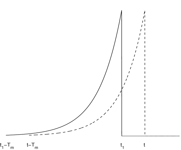
FIG. 1.: Diagram of the weighting distribution over the times of emission for a particle that may be detected in the output at time $t$ (dashed line) and that has been detected at time $t_{1}$ (solid line). The times at which previous emissions can be neglected $t-T_{\rm m}$ and $t_{1}-T_{\rm m}$ are also shown.

FIG. 2.: Schematic of the spectral detection setup. The output from the system of interest is an input to one of the spectrometer channels. The inputs to the other channels are simply the vacuum. The spectrometer mixes the channel inputs so that the output channels contain certain spectral components of the original system output (as well as contributions from the other channel inputs).

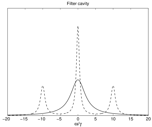
FIG. 3.: Schematic of the filtering situation considered. The three peaked spectrum of the two level atom is shown and superimposed on top is the Lorentzian lineshape of the Fabry Perot filter. The filter cavity is on resonance with the atomic transition $\nu=0$ (the central peak of the Mollow spectrum) and has a line width larger than the atomic decay rate, $\kappa=5\gamma$. The side peaks of the Mollow spectrum are at $\pm\Omega$, where $\Omega=10\gamma$.

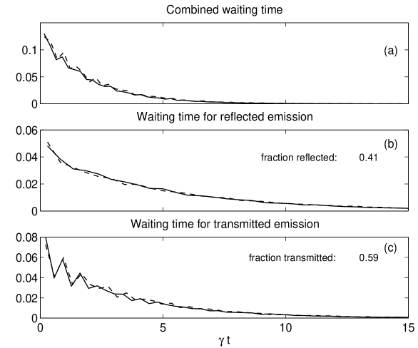
FIG. 4.: Plot of the results of a simulation of the filtering situation depicted in Fig.3, all three plots are waiting time distributions (in arbitrary units) determined by bining the times between each subsequent detection in 100 bins. The solid line is from the non-Markovian quantum trajectory, the dashed line is the Markovian method for the extended system. (a) is a plot of the combined photodetection waiting time distribution from both the reflected and transmitted emission. (b) shows the waiting time distribution for just the reflected emission (which consists mostly of the two side peaks). (c) is a plot of the waiting time distribution for the transmitted emission (mostly from the central peak).The ratio of the transmitted and reflected emission is also given.

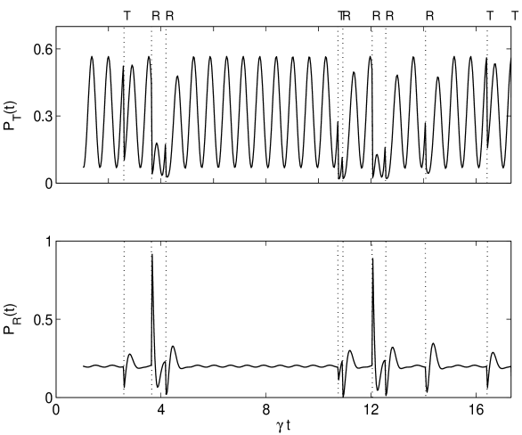
FIG. 5.: Plot of the probabilities for detecting a transmitted $P_{T}$ and reflected $P_{R}$ photon during the evolution of a single quantum trajectory for the first ten detections. The labels $R$ for reflected and $T$ for transmitted at the top of the graph denote the channel that the detection occurred in and the dotted vertical lines indicate the time of the detections.

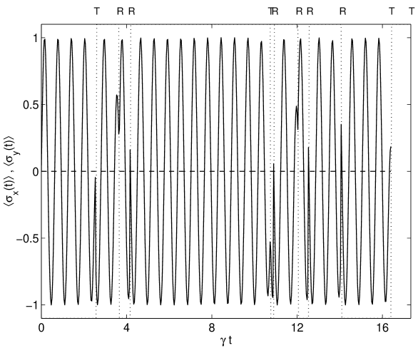
FIG. 6.: Plot of the conditioned expectation values for $\sigma_{y}$ (solid line) and $\sigma_{x}$ (dashed line) for the same trajectory as in Fig.5.

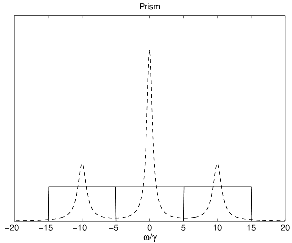
FIG. 7.: Schematic of the prism-like spectral detection situation. The three peaked spectrum of the two level atom is shown and superimposed on top are the top-hat functions corresponding to the detectors centered on each peak. The spread of the frequency band of each channel is $\Delta/2=5\gamma$ and $\omega_{L}=-\Omega$, $\omega_{R}=+\Omega$ and $\omega_{C}=0$, where, as before, $\Omega=10\gamma$.

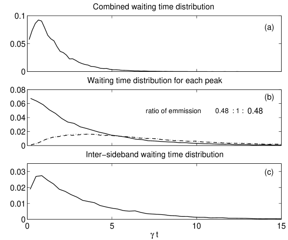
FIG. 8.: Plot of the results of a simulation of the prism depicted in Fig.7, all three plots are waiting time distributions determined by bining the times between each subsequent detection in 100 bins. (a) is a plot of the combined photodetection waiting time distribution from all three spectral bands, (compare with Fig.4 (a)). (b) shows the waiting time distributions within each spectral band (each band coinciding with one peak of the emission). The solid line corresponds to the central peak and the dashed and dotted lines to the side-peaks. (c) is a plot of the inter-sideband waiting time distribution, i.e., the time taken between a detection in one of the side peaks and a detection in the other. The ratio of the emission into each peak is also shown

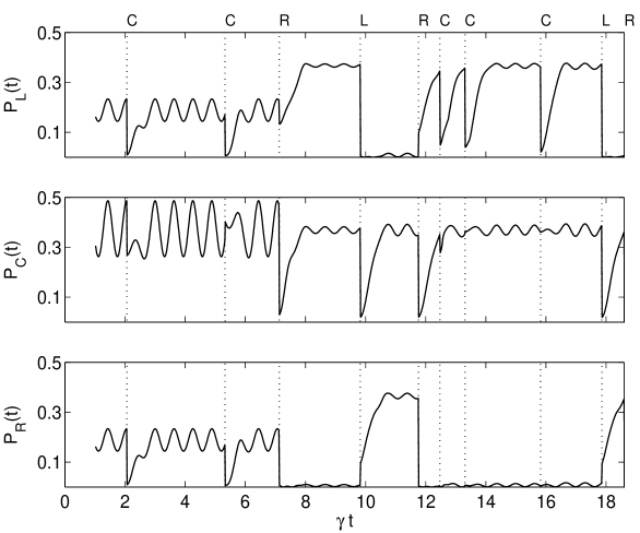
FIG. 9.: Plot of the probabilities for detecting a photon from the central peak $P_{C}$ and the two side peaks $P_{L}$ and $P_{R}$ during the evolution of a single quantum trajectory for the first ten detections. The labels $C$ for central and $L$ and $R$ for the side-peaks at the top of the graph denote the channel that the detection occurred in and the dotted vertical lines indicate the time of the detections.

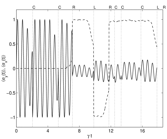
FIG. 10.: Plot of the conditioned expectation values of $\sigma_{y}$ (solid line) and $\sigma_{x}$ (dashed line) for the same trajectory as depicted in Fig.9.

REFERENCES

- [1] J. Dalibard, Y. Castin, and K. Mølmer, Phys. Rev. Lett. 68, 580 (1992).
- [2] H. Carmichael, An Open Systems Approach to Quantum Optics, Lecture Notes in Physics m18 (Springer-Verlag, New York, 1991).
- [3] N. Gisin and I. Percival, Phys. Lett. 167A (1992).
- [4] C. W. Gardiner A. S. Parkins and P. Zoller Phys. Rev. A, 46, 4363 (1992).
- [5] K. Mølmer, Y. Castin and J. Dalibard, J. Opt. Soc. Am. B 10, 524 (1993).
- [6] R. Dum, P. Zoller and H. Ritsch, Phys. Rev. A 45, 4879 (1992).
- [7] L. Tian and H. J. Carmichael, Phys. Rev. A, 46, R6801 (1992).
- [8] M. D. Srinivas and E. B. Davies, Opt. Acta 28, 981 (1981).
- [9] H. M. Wiseman and G. J. Milburn, Phys. Rev. A 47, 642 (1993).
- [10] P. Goetsch and R. Graham, Phys. Rev. A 50, 5242 (1994).
- [11] J. Javanainen and S. M. Yoo Phys. Rev. Lett. 76, 161 (1996).
- [12] S. Bay, P. Lambropoulos and K. Mølmer, Phys. Rev. Lett. 79, 14 (1997).
- [13] N. Vats and S. John, (unpublished).
- [14] M. O. Mewes et al., Phys. Rev. Lett. 78, 582 (1997).
- [15] J. Hope, Phys. Rev. A 55, R2531, (1997).
- [16] G. M. Moy, J. J. Hope and C. M. Savage, (unpublished).
- [17] C. M. Caves, Phys. Rev. D 35, 1815 (1986).
- [18] A. Barchielli, Phys.Rev. D 34, 2527 (1986).
- [19] H. M. Wiseman, Ph.D. Thesis, University of Queensland (1994).
- [20] C. Cohen-Tannoudji and S. Reynaud, Phil. Trans. R. Soc. Lond. A 293, 223 (1979).
- [21] J. D. Cresser, J. Phys. B: At. Mol. Phys. 20, 4915 (1987).
- [22] H. M. Wiseman and G. J. Milburn, Phys. Rev. A 47, 1652 (1993).
- [23] A. Imamoḡlu, Phys. Rev. A 50, 3650 (1994).
- [24] L. Diòsi and W. T. Strunz, Phys. Lett. A 235, 569 (1997).
- [25] L. Diòsi, N. Gisin and W. T. Strunz, (unpublished).
- [26] B. R. Mollow, Phys. Rev. 188, 1969 (1969).
- [27] A. Aspect, G. Roger, S. Reynaud, J. Dalibard, and C. Cohen-Tannoudji, Phys. Rev. Lett. 45, 617 (1980).
- [28] C. W. Gardiner, Phys. Rev. Lett. 70, 2269 (1993)
- [29] H. J. Carmichael, Phys. Rev. Lett. 70, 2273 (1993). (1996).
- [30] E. B. Davies, Quantum Theory of Open Systems, (Academic Press, London, 1976).
- [31] C. W. Gardiner, Quantum Noise, Springer series in synergetics (Springer-Verlag, New York,1991).
- [32] C. W. Gardiner and M. J. Collett, Phys. Rev. A 31, 3761 (1985).
- [33] S. D. Stearns and D. R. Hush, Digital Signal Analysis 2nd ed., Prentice Hall Signal Processing Series, (Prentice Hall, New Jersey, 1990)
- [34] D. F. Walls and G. J. Milburn, Quantum Optics (Springer-Verlag, New York, 1994).