Unraveling quantum dissipation in the frequency domain

Abstract

We present a quantum Monte Carlo method for solving the evolution of an open quantum system. In our approach, the density operator evolution is unraveled in the frequency domain. Significant advantages of this approach arise when the frequency of each dissipative event conveys information about the state of the system.

Irreversibility may be incorporated in quantum theory by coupling a system to a Markoffian reservoir and tracing over the reservoir (corresponding to averaging over unobserved quantities) to give a description of the system evolution by a reduced density operator equation. Recently, a number of theoretical methods have been developed which do not perform this trace, but consider instead a single trial (quantum trajectory) in which the reservoir is continuously monitored [1, 2, 3, 4, 5]. Each such trial is conditional on a sequence of times $t_{1}$, $t_{2}$, $\ldots$, for the dissipation events where each $t_{n}$ may be in general associated with a decay channel $\gamma_{n}$. For example, in the case of spontaneous emission from an atom, $\gamma_{n}$ would identify a unique polarization and direction for the photon. Apart from providing valuable insight into the underlying quantum dynamics, there are significant numerical advantages for evolving wave functions rather than reduced density operators, and consequently these methods have already received widespread application.

The decomposition of the density operator evolution to form a parallel set of quantum trajectories is not unique since there are always degrees of freedom associated with the quantum measurement basis used to record the excitations of the reservoir. Significantly, both the insight one is able to gain into the dynamics of the system as well as the efficiency of the resulting numerical algorithm can be very sensitive to this choice. In this letter, we derive the theory of quantum trajectories (closely related to quantum Monte Carlo simulations) in which the unraveling is done in the frequency domain rather than performing the decomposition in time. Consequently, the characteristic features of previous approaches such as quantum jumps of the state and quantum state diffusion are not present. Instead we find the observables of the system evolve according to a continuous evolution.

The essential idea is to replace the observed decay times $t_{n}$ by frequencies $\omega_{n}$. Each quantum trajectory is then conditional on a particular record of the reservoir state $\omega_{1}$, $\omega_{2}$, $\ldots$, produced by a fictitious measurement device of the type illustrated in Fig. 1. The output of the quantum system is sorted by a cascaded array of filters which allow only a particular frequency component of the field to pass onto each detector. The unavoidable consequence of the filters is that associating a frequency with each dissipative event requires that knowledge of the precise time at which each decay occurred is lost. If we consider a time interval $t\in[0,\tau]$, in order to form a complete reservoir description according to the Fourier sampling theorem, each $\omega_{i}$ must be chosen from a discrete but infinite set of frequencies, spaced $2\pi/\tau$ apart.

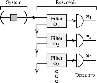
FIG. 1.: The frequency measurement detector. Each output channel of the system is sorted by a cascaded array of filters.

As we will now show, these novel quantum trajectories are straight forward to derive. In the case of the measurement record corresponding to no decays, the choice of the time domain or the frequency domain is irrelevant. We let $\bigl{|}0_{R}\bigr{>}$ be the vacuum state in the space of the reservoir and denote the state of both and system and reservoir by $\bigl{|}\Psi(t)\bigr{>}$. The quantum trajectory corresponding to no decays $\bigl{|}\psi(t)\bigr{>}=\bigl{<}0_{R}\bigm{|}\Psi(t)\bigr{>}$ evolves according to

$${d\bigl{|}\psi(t)\bigr{>}\over dt}={1\over i\hbar}H_{\rm eff}\bigl{|}\psi(t)\bigr{>}$$ (1)

in which the non-Hermitian Hamiltonian $H_{\rm eff}$ is related to the Hamiltonian for the isolated system $H_{\rm sys}$ by

$$H_{\rm eff}=H_{\rm sys}-{i\hbar\over 2}\sum_{\gamma}a_{\gamma}^{{\dagger}}a_{\gamma}.$$ (2)

The operators $a_{\gamma}$ (called jump operators in the quantum Monte Carlo approach) act in the system space and induce the corresponding change in the system state when a decay into channel $\gamma$ occurs.

To treat one decay, we introduce the filter operator for a single frequency $\omega_{1}$ in channel $\gamma_{1}$ [5]

$$r_{\omega_{1}}(t)={1\over\sqrt{\tau}}\int_{0}^{t}e^{-i\omega_{1}(t-s)}\,dF_{\gamma_{1}}(s)$$ (3)

where the field operator $dF_{\gamma_{1}}(s)$ acts in the reservoir space and annihilates one excitation in the mode $\gamma_{1}$ in the time interval $s$ to $s+ds$. The quantum trajectory is found by applying $r_{\omega_{1}}(t)$ to $\bigl{|}\Psi(t)\bigr{>}$ and then projecting the filtered state onto the vacuum to enforce one decay

$$\bigl{|}\psi_{\omega_{1}}(t)\bigr{>}=\bigl{<}0_{R}\bigr{|}r_{\omega_{1}}(t)\bigl{|}\Psi(t)\bigr{>}.$$ (4)

The equation of motion for this is coupled to the evolution of $\bigl{|}\psi(t)\bigr{>}$ by (see Eq. (153) of Ref. [5])

$${d\over dt}\bigl{|}\psi_{\omega_{1}}(t)\bigr{>}={a_{\gamma_{1}}\over\sqrt{\tau}}\bigl{|}\psi(t)\bigr{>}+{1\over i\hbar}(H_{\rm eff}+\hbar\omega_{1})\bigl{|}\psi_{\omega_{1}}(t)\bigr{>}$$ (5)

For two or more decays, one may proceed in different directions depending on whether or not time ordering is imposed on the dissipative events. We first consider the rules for deriving the trajectory in the case of unordered measurements $(u)$. This is the situation applicable for the device shown in Fig. 1 where the order of the frequencies in the record list plays no role. The associated quantum trajectory is defined as

$$\bigl{|}\psi^{(u)}_{\omega_{1},\ldots,\omega_{n}}(t)\bigr{>}=\bigl{<}0_{R}\bigr{|}r_{\omega_{1}}(t)\ldots r_{\omega_{n}}(t)\bigl{|}\Psi(t)\bigr{>}$$ (6)

which evolves according to

$${d\over dt}\bigl{|}\psi^{(u)}_{\omega_{1},\ldots,\omega_{n}}(t)\bigr{>} =\sum_{p=1}^{n}{a_{\gamma_{p}}\over\sqrt{\tau}}\bigl{|}\psi^{(u)}_{\omega_{1},\ldots,\omega_{p-1},\omega_{p+1},\ldots,\omega_{n}}(t)\bigr{>}$$ (8)

$$+{1\over i\hbar}\Bigl{(}H_{\rm eff}+\hbar\sum_{p=1}^{n}\omega_{p}\Bigr{)}\bigl{|}\psi^{(u)}_{\omega_{1},\ldots,\omega_{n}}(t)\bigr{>}$$

The first summation couples the trajectory to all $n$ trajectories which exclude one of the frequencies in the list by the associated jump operator for that decay. Note that Eq. (5) is a special case of Eq. (8) with $n=1$. Although the evolution of any trajectory can be found by iterating Eq. (8) back to Eq. (1), the number of coupled equations which must be solved grows as $2^{n}$. Consequently it is difficult to treat long time intervals $\tau$ in which a large number of decays may occur in this way.

The scaling is more favorable in the case of time ordered decays $(o)$ which we now consider. In this case we impose the constraint that the $\omega_{1}$ decay occurs before the $\omega_{2}$ decay, which occurs before the $\omega_{3}$ decay, and so on. Since this corresponds to a different physical measurement (e.g. an atomic cascade), the quantum trajectories are distinct from those of the unordered case. The corresponding nested filter operators are defined recursively starting from Eq. (3) by

$$r_{\omega_{1},\ldots,\omega_{n}}(t)={1\over\sqrt{\tau}}\int_{0}^{t}r_{\omega_{1},\ldots,\omega_{n-1}}(s)\,e^{-i\omega_{n}(t-s)}\,dF_{\gamma_{n}}(s)$$

The trajectories in this case are

$$\bigl{|}\psi^{(o)}_{\omega_{1},\ldots,\omega_{n}}(t)\bigr{>}=\bigl{<}0_{R}\bigr{|}r_{\omega_{1},\ldots,\omega_{n}}(t)\bigl{|}\Psi(t)\bigr{>}$$ (9)

and evolve according to

$${d\over dt}\bigl{|}\psi^{(o)}_{\omega_{1},\ldots,\omega_{n}}(t)\bigr{>} ={a_{\gamma_{n}}\over\sqrt{\tau}}\bigl{|}\psi^{(o)}_{\omega_{1},\ldots,\omega_{n-1}}(t)\bigr{>}$$ (11)

$$+{1\over i\hbar}\Bigl{(}H_{\rm eff}+\hbar\sum_{p=1}^{n}\omega_{p}\Bigr{)}\bigl{|}\psi^{(o)}_{\omega_{1},\ldots,\omega_{n}}(t)\bigr{>}$$

The difference between this and Eq. (8) is that here the evolution of each trajectory is coupled only to the trajectory which excludes the last measurement in the list via the jump operator for that decay. The number of coupled equations which must be solved is equal to $n+1$. In Fig. 2 we illustrate the solution of this for a few sample trajectories for the case of resonance fluorescence from a two-level atom. For this case $H_{\rm sys}=\hbar\Omega(\sigma^{+}+\sigma^{-})/2$ where $\sigma^{+}$ and $\sigma^{-}$ are the usual raising and lowering operators and $\Omega$ is the Rabi frequency. The single jump operator $\sqrt{\Gamma}\sigma^{-}$ defines the spontaneous emission rate $\Gamma$.

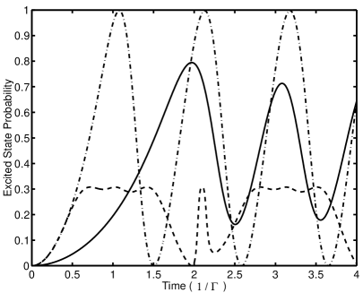
FIG. 2.: Sample quantum trajectories $\bigl{|}\psi_{9\Gamma}(t)\bigr{>}$ (dashed), $\bigl{|}\psi_{0.3\Gamma}(t)\bigr{>}$ (dash-dot), and $\bigl{|}\psi_{3\Gamma,0.5\Gamma,-0.3\Gamma}(t)\bigr{>}$ (solid), for resonance fluorescence from a two-level atom with $\Omega=6\Gamma$.

This recipe allows us to calculate arbitrary trajectories in both cases, but it remains to show that it represents a correct physical unraveling of the reduced density operator equation. This is most easily done with the identity

$$\sum_{\omega_{n}}\bigl{|}\psi_{\omega_{1},\ldots,\omega_{n}}(t)\bigr{>}={\sqrt{\tau}\over 2}a_{\gamma_{n}}\bigl{|}\psi_{\omega_{1},\ldots,\omega_{n-1}}(t)\bigr{>}$$ (12)

which may be proved for both unordered and ordered trajectories using Eq. (6) or Eq. (9) to expand the left hand side, evaluating the $\omega_{n}$ summation to give the Dirac delta function, and applying Eq. (81) of Ref. [5]. The reduced density operator is constructed by tracing over all possible measurement records

$$\rho=\sum_{n=0}^{\infty}\Bigl{[}\sum_{\omega_{1}}\ldots\sum_{\omega_{n}}\rho_{\omega_{1},\ldots,\omega_{n}}\Bigr{]}$$ (13)

where $\rho_{\omega_{1},\ldots,\omega_{n}}$ is

$$\left\{\begin{array}[]{l@{\hspace{1pc}}l}\bigl{(}\bigl{|}\psi^{(u)}_{\omega_{1},\ldots,\omega_{n}}(t)\bigr{>}\bigl{<}\psi^{(u)}_{\omega_{1},\ldots,\omega_{n}}(t)\bigr{|}\bigr{)}/n!\hfil\hskip 12.0pt&{\rm unordered}\\[5.0pt] \bigl{|}\psi^{(o)}_{\omega_{1},\ldots,\omega_{n}}(t)\bigr{>}\bigl{<}\psi^{(o)}_{\omega_{1},\ldots,\omega_{n}}(t)\bigr{|}\hfil\hskip 12.0pt&{\rm ordered}\end{array}\right.$$ (14)

The $n!$ arises from the trivial permutations of $n$ frequencies which correspond to the same trajectory. Differentiating Eq. (13) with respect to time, and using Eq. (12) along with either Eq. (8) or Eq. (11) gives in both cases the same equation for $\rho$

$${d\rho\over dt}\!\!=\!\!{1\over i\hbar}[H_{\rm sys},\rho]+{1\over 2}\sum_{\gamma}(2a_{\gamma}\rho a_{\gamma}^{{\dagger}}-a_{\gamma}^{{\dagger}}a_{\gamma}\rho-\rho a_{\gamma}^{{\dagger}}a_{\gamma})$$ (15)

which is the quantum master equation [6]. This is the key result, and it implies that the frequency domain method we have presented is a correct unraveling of the reduced density operator at all times.

As is the case in the time domain, the ensemble formed by a large but finite set of trajectories, will approximate the result of the complete trace and yet involve the evolution of wave functions rather than density operators. We now outline the simulation procedure we have adopted focusing on the case of ordered trajectories. Specifically we would like to calculate the evolution of an arbitrary observable of the system $\bigl{<}{\cal O}\bigr{>}={\rm Tr}\{{\cal O}\rho\}$ using frequency unraveling. The procedure is as follows

1. Select a system state $\bigl{|}\psi(0)\bigr{>}$ from the initial statistical mixture in $\rho$ (trivial if $\rho$ is a pure state) and calculate the zero trajectory $\bigl{|}\psi(t)\bigr{>}$ from Eq. (1).

2. Construct the one decay trajectories $\bigl{|}\psi_{\omega_{1}}(t)\bigr{>}$ coupled to this with $\omega_{1}$ taking on all values from a discrete set, $\{2\pi p/\tau\}$ for $p$ integer.

3. Using a random number, select a value for $\omega_{1}$ weighted by the normalization of the trajectories at time $\tau$, i.e. from the probability distribution

   $$P(\omega_{n})={\bigl{<}\psi_{\omega_{1},\ldots,\omega_{n}}(\tau)\bigm{|}\psi_{\omega_{1},\ldots,\omega_{n}}(\tau)\bigr{>}\over\sum_{\omega_{n}}\bigl{<}\psi_{\omega_{1},\ldots,\omega_{n}}(\tau)\bigm{|}\psi_{\omega_{1},\ldots,\omega_{n}}(\tau)\bigr{>}}$$ (16)

   with $n=1$ here for the first decay.

4. Construct $\bigl{|}\psi^{(o)}_{\omega_{1},\omega_{2}}(t)\bigl{>}$ with $\omega_{1}$ fixed and with $\omega_{2}$ varying over all values given in the discrete set. Select a value for $\omega_{2}$ using Eq. (16) with $n=2$.

5. Continue, selecting a frequency for each decay, until a predetermined maximum number is reached.

6. Since we perform a partial evaluation of the series in Eq. (13), the estimate for $\bigl{<}{\cal O}\bigr{>}$ is a weighted sum over those trajectories which are calculated

   $$\sum_{\rm traj}P^{-1}_{\rm traj}\bigl{<}\psi^{(o)}_{\omega_{1},\ldots,\omega_{n}}(t)\bigr{|}{\cal O}\bigl{|}\psi^{(o)}_{\omega_{1},\ldots,\omega_{n}}(t)\bigr{>}$$ (17)

   where $P_{\rm traj}$ is the probability of the trajectory being evaluated in the algorithm. This probability $P_{\rm traj}$ is unity for the zero and all the one decay trajectories which are always calculated, equal to $P(\omega_{1})$ for the two decay trajectories, $P(\omega_{1})P(\omega_{2})$ for the three decay trajectories, and so on.

7. Start again from the beginning and average the results from many such trials to form the ensemble.

A simple check of the numerical implementation is to establish that ${\rm Tr}\{\rho\}=1$ (for ${\cal O}=1$) at all time. In Fig. 3 we apply this approach to form the ensemble time evolution for the case of resonance fluorescence.

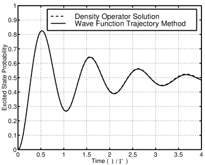
FIG. 3.: Monte Carlo simulation with 2500 trials for resonance fluorescence from a two-level atom with $\Omega=6\Gamma$.

Since our method is based on frequency measurement, the calculation of spectra arises naturally by bining the frequencies of the trajectories in the simulation. For example, we outline now the procedure for using time ordered trajectories to calculate the fluctuation spectrum

$$S_{\gamma}(\omega) = \lim_{t\to\infty}\int_{0}^{t}\int_{0}^{t}e^{-i\omega(s-s^{\prime})}\bigl{<}\Psi\bigr{|}dF_{\gamma}^{{\dagger}}(s)dF_{\gamma}(s^{\prime})\bigl{|}\Psi\bigr{>}$$ (18)

$$= \lim_{t\to\infty}\bigl{<}\Psi\bigr{|}r^{{\dagger}}_{\omega}(t)r_{\omega}(t)\bigl{|}\Psi\bigr{>}$$ (19)

which is the rate of decay of frequency $\omega$ in channel $\gamma$. We define a partially ordered trajectory $(p)$

$$\bigl{|}\psi^{(p)}_{\omega_{1},\ldots,\omega_{n};\omega}(t)\bigr{>}=\bigl{<}0_{R}\bigr{|}r_{\omega}(t)r_{\omega_{1},\ldots,\omega_{n}}(t)\bigl{|}\Psi(t)\bigr{>}$$ (20)

which evolves according to

$${d\over dt}\bigl{|}\psi^{(p)}_{\omega_{1},\ldots,\omega_{n};\omega}(t)\bigr{>}=$$ (21)

$$\qquad{a_{\gamma}\over\sqrt{\tau}}\bigl{|}\psi^{(o)}_{\omega_{1},\ldots,\omega_{n-1}}(t)\bigr{>}+{a_{\gamma_{n}}\over\sqrt{\tau}}\bigl{|}\psi^{(p)}_{\omega_{1},\ldots,\omega_{n-1};\omega}(t)\bigr{>}$$ (22)

$$\qquad+{1\over i\hbar}\Bigl{(}H_{\rm eff}+\hbar\sum_{p=1}^{n}\omega_{p}+\hbar\omega\Bigr{)}\bigl{|}\psi^{(p)}_{\omega_{1},\ldots,\omega_{n};\omega}(t)\bigr{>}$$ (23)

The calculation proceeds in exactly the same way as previously outlined except for step 6 which becomes

1. When calculating $\bigl{|}\psi^{(o)}_{\omega_{1},\ldots,\omega_{n}}(t)\bigr{>}$ with $\omega_{n}$ varying over all values from the discrete set, evaluate also $\bigl{|}\psi^{(p)}_{\omega_{1},\ldots,\omega_{n-1};\omega_{n}}(t)\bigr{>}$. The estimate for $S_{\gamma}(\omega_{n})$ is

   $$\sum_{\rm traj}P_{\rm traj}^{-1}\bigl{<}\psi^{(p)}_{\omega_{1},\ldots,\omega_{n-1};\omega_{n}}(\tau)\bigm{|}\psi^{(p)}_{\omega_{1},\ldots,\omega_{n-1};\omega_{n}}(\tau)\bigr{>}$$

   where $P_{\rm traj}$ is identical to the previous case.

This computes a transient spectrum unless the steady state density operator is used for the initial condition. Since $\tau$ is finite, it should replace the upper limit of both integrals in Eq. (19) which is equivalent to simulating the spectrum $S_{\gamma}(\omega)$ convolved with $(\tau/2\pi){\rm sinc}^{2}(\omega\tau/2\pi)$. This is intuitive since one would expect a long $\tau$ to be required to achieve high frequency resolution. In Fig. 4, we have applied this to calculate the Mollow spectrum [7].

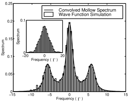
FIG. 4.: Comparison of the simulated wave function spectrum with the Mollow spectrum convolved with $(\tau/2\pi){\rm sinc}^{2}(\omega\tau/2\pi)$ for $\tau=4/\Gamma$ and $\Omega=6\Gamma$. The inset shows the same comparison for the short time $\tau=1/\Gamma$ where the sidebands cannot be resolved.

Unraveling the density operator equation to form quantum trajectories is of significance for a number of reasons. When the system space is large it can be impossible to computationally store and evolve the density matrix and one is then forced to use quantum trajectory methods which require only the simulation of wave functions. The more fundamental aspect [8, 9, 10] is that the system evolution is conditional on the reservoir record and when an appropriate measurement basis is used, the system may be continuously localized to a region of its Hilbert space. The key requirement for this is that the dissipative events must provide information about the system state. A simple example is in the case of spontaneous emission where imaging the source of the photon allows one to localize the position wave function of the atom and use a reduced basis set to track the atomic motion [10].

We have presented in this Letter the measurement basis which identifies the energy of dissipative events; an intrinsically different kind of information to the time domain approaches. There are numerous examples of physical systems in which this information is of interest e.g. radiative heating in ultracold collisions [11] (where the frequency of photons is correlated with the internuclear separation) and laser cooling [12] (where as the atomic gas cools photons of higher frequency than the driving fields are emitted). We have illustrated here the calculation of the fluctuation spectrum, although ordered spectra may also have intrinsic interest for certain problems. A final point of note is that the total evolution time may be partitioned into intervals of width $\tau$ and each solved using the method we have presented. Then varying $\tau$ one can sweep continuously between use of the time and frequency domains.

We would like to thank J. Cooper for helpful discussions. This work was supported by the NSF.

REFERENCES

- [1] A. Barchielli and V. P. Belavkin, J. Phys. A 24, 1495 (1991).
- [2] J. Dalibard, Y. Castin, and K. Molmer, Phys. Rev. Lett. 68, 580 (1992).
- [3] H. J. Carmichael, An Open Systems Approach to Quantum Optics (Springer, Berlin, 1993).
- [4] N. Gisin and I. C. Percival, J. Phys. A, 25, 5677 (1992).
- [5] C. W. Gardiner, A. S. Parkins, and P. Zoller, Phys. Rev. A 46 4363 (1992).
- [6] C. Gardiner, Quantum Noise (Springer, Berlin, 1991).
- [7] B. R. Mollow, Phys. Rev. A 12, 1919 (1975).
- [8] N. Gisin and I.C. Percival, Phys. Lett. A 167, 315 (1992).
- [9] B. M. Garraway and P. L. Knight, Phys. Rev. A49, 1266 (1994).
- [10] M. Holland, S. Marksteiner, P. Marte, and P. Zoller, Phys. Rev. Lett. 76, 3683 (1996).
- [11] M. J. Holland, K.-A. Suominen, and K. Burnett, Phys. Rev. Lett. 72 2367 (1994).
- [12] K. Molmer, Y. Castin, and J. Dalibard, J. Opt. Soc. Am. B bf 10 524 (1993).