Retroactive quantum jumps in a strongly-coupled atom–field system

Abstract

We investigate a novel type of conditional dynamic that occurs in the strongly-driven Jaynes-Cummings system with dissipation. Extending the work of Alsing and Carmichael [Quantum Opt. 3, 13 (1991)], we present a combined numerical and analytic study of the Stochastic Master Equation that describes the system’s conditional evolution when the cavity output is continuously observed via homodyne detection, but atomic spontaneous emission is not monitored at all. We find that quantum jumps of the atomic state are induced by its dynamical coupling to the optical field, in order retroactively to justify atypical fluctuations occurring in the homodyne photocurrent.

Quantum trajectory theories [1, 2, 3, 4] have proven to be of paramount importance in contemporary quantum optics. This is largely because they provide powerful computational tools for predicting the correlation functions and optical spectra of systems with many active degrees of freedom. However, quantum trajectories have recently begun to play an equally important role as the essential theoretical basis for describing conditional evolution of continuously-observed open quantum systems.

In this Letter, we use the Stochastic Master Equation (SME) formalism developed in Ref. [2] to reveal a new type of conditional-dynamical phenomenon that occurs in a strongly-coupled open quantum system under partial observation. We call this phenomenon retroactive quantum jumps. We believe that this work represents the first use of a measurement-based SME in analyzing a dynamical behavior specific to partially-observed systems. Our analysis also illustrates the utility of more traditional approaches, in particular the use of the Glauber-Sudarshan $P\left(\alpha\right)$-function [5], in deriving simplified conditional evolution equations that retain all the essential features of a system’s quantum dissipative dynamics.

The particular physical system we have studied is the driven Jaynes-Cummings model [6] with dissipation [1, 7]. This consists of a two-level atom resonantly coupled to a resonantly driven cavity mode. The two output channels for this system are atomic spontaneous emission into non-cavity optical modes (at an overall rate of $2\gamma_{\perp}$), and leakage of photons from the cavity mode through an output-coupling mirror (at rate $2\kappa$). We focus on the strong atom-cavity coupling limit $g\gtrsim\kappa,\gamma_{\perp}$, and also assume a strong driving field $E$. The optical input-output relations for an atom-cavity system of this type have been experimentally investigated in Refs. [8, 9].

In a frame rotating at the driving laser frequency, the unconditional master equation is

$$\dot{\rho}=[g(a^{\dagger}\sigma-\sigma^{\dagger}a)-iEy,\rho]+2\kappa{\cal D}[a]\rho+2\gamma_{\perp}{\cal D}[\sigma]\rho.$$ (1)

Here, for arbitrary operators $A$ and $B$, ${\cal D}[A]B=A^{\dagger}BA-\mbox{$\frac{1}{2}$}\{A^{\dagger}A,B\}$, and $y\equiv-ia+ia^{\dagger}$ is the phase quadrature of the field (so that $x\equiv a+a^{\dagger}$ is the amplitude quadrature), and $\sigma=|{g}\rangle\langle{e}|$ is the lowering operator for the atom.

A lot of insight can be gained into this problem by considering the corresponding classical equations of motion [10]. This is done by using the master equation (1) to calculate the time derivatives of the variables

$$\alpha=\langle{a}\rangle\;,\;\;s=\langle{\sigma}\rangle\;,\;\;w=\langle{\sigma_{z}}\rangle=\langle{[\sigma^{\dagger},\sigma]}\rangle,$$ (2)

then factorizing all field-atom operator products. If we ignore spontaneous emission by setting $\gamma_{\perp}=0$, we find that the atom will remain in a pure state with $w^{2}+4|s|^{2}=1$. Then for $2E>g$ this system has just two fixed points [10]

$$\alpha_{\pm}^{\rm fix}=\frac{E+gs^{\rm fix}_{\pm}}{\kappa}\;,\;\;s_{\pm}^{\rm fix}=-\frac{g}{4E}\mp i\left[{\frac{1}{4}-\left(\frac{g}{4E}\right)^{2}}\right]^{1/2}$$ (3)

with $w^{\rm fix}=0$. That is, the phase of the field is correlated with the state of the atom (which is fully polarized).

In the high driving limit $E\gg g$ (which can be quite realistic), these expressions simplify and the two fixed points correspond to orthogonal quantum states:

$$|{\psi^{\rm fix}_{\pm}}\rangle=|{\alpha_{\pm}^{\rm fix}}\rangle|{\pm}\rangle\equiv|{\alpha_{\pm}^{\rm fix}}\rangle 2^{-1/2}\left[|{g}\rangle\mp i|{e}\rangle\right],$$ (4)

where $|{\alpha_{\pm}^{\rm fix}}\rangle$ is the coherent state with amplitude

$$\alpha_{\pm}^{\rm fix}=E/\kappa\mp i(g/2\kappa)\equiv\bar{\alpha}\mp i(g/2\kappa).$$ (5)

The purity of the atomic state is not preserved if we put back spontaneous emission. Nevertheless, if $\gamma_{\perp}$ is small, then the density operator will tend towards an equal mixture of the two states $|{\psi^{\rm fix}_{\pm}}\rangle$ [10]. We have confirmed this by numerically finding the stationary solution of Eq. (1), which has a bimodal $Q\left(\alpha\right)$-function as shown in Fig. 1.

Our aim is to elucidate the quantum dissipative dynamics that generate this bimodal distribution, in particular the formal mechanisms that enforce correlations between atomic state and optical phase when the system is subjected to partial (but continuous) observation.

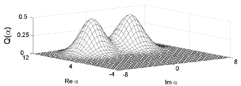
FIG. 1.: Steady-state $Q(\alpha)$-function for the master equation (1), with parameters as in Fig. 2.

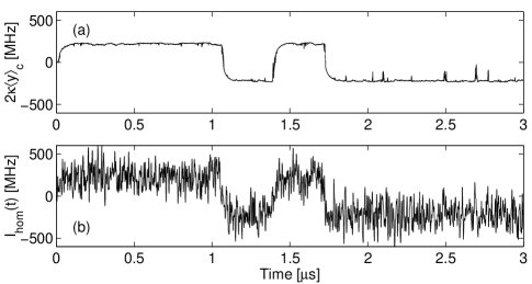
FIG. 2.: Simulation of the master equation (1) with the stochastic term Eq. (9) added (see text for parameters). (a) conditional $\langle{y}\rangle$; (b) homodyne photocurrent as in Eq. (10).

To achieve this aim we first simplify Eq. (1) using a method related to that of Ref. [10]. We first transform to an interaction picture with respect to the Hamiltonian

$$H_{0}=ig\bar{\alpha}(\sigma-\sigma^{\dagger})\equiv i(\Omega/2)(\sigma-\sigma^{\dagger}).$$ (6)

In this picture $\sigma(t)=(-i/2)(\mu e^{-i\Omega t}+\mu_{z}-\mu^{\dagger}e^{i\Omega t})$, where $\mu=|{-}\rangle\langle{+}|$ and $\mu_{z}=[\mu^{\dagger},\mu]$. Then, assuming that $\Omega$ is much greater than the characteristic rates of atomic evolution $\gamma,g,g^{2}/\kappa$, we can make a rotating wave approximation for frequency $\Omega$ to derive

$$\dot{\rho} = -i[Ey+(g/2)\mu_{z}x,\rho]+2\kappa{\cal D}[a]\rho$$ (8)

$$+\,(\gamma_{\perp}/2)\left\{{\cal D}[\mu]+{\cal D}[\mu_{z}]+{\cal D}[\mu^{\dagger}]\right\}\rho.$$

Here the atomic spontaneous emission has been split into three decay channels corresponding respectively to the upper, middle and lower peaks of the Mollow triplet.

Alsing and Carmichael, who derived a master equation similar to Eq. (8), showed that a quantum trajectory unraveling based on detecting the three different photon frequencies would force the coupled atom-field state into a pure state of the form $|{\pm}\rangle|{\alpha}\rangle$ [10]. Here the coherent amplitude $\alpha$ of the field evolves smoothly between jumps that change the atomic state. Between jumps the field state is attracted to the fixed point $\alpha_{\pm}^{\rm fix}$ corresponding to the current atomic state $|\pm\rangle$. If $\gamma_{\perp}\ll\kappa$, then on a long time scale these are occupied with equal probability.

While the unraveling based on observation of atomic decays provides an intuitive picture of the dynamics, high-efficiency frequency-resolved monitoring of atomic fluorescence is not yet experimentally feasible. Given the strong correlation between atomic state and optical phase, however, it should be possible to observe state-changing atomic decays ‘indirectly’ via homodyne monitoring of the phase-quadrature of the cavity output. This would be much easier to implement in the laboratory. One would expect to see bistability of the field with values $\alpha_{\pm}^{\rm fix}$, with stochastic switching induced (according to the intuitive picture outlined above) by atomic spontaneous emission. But from a theoretical perspective, we must now ask how jump-like behavior could emerge from the evolution equations for a situation in which no counting or projective measurements are assumed to be made. In what sense should we be able to associate observed phase-switching events with ‘actual’ atomic decays?

From the theory of Ref. [2], homodyne monitoring of the cavity output can be modeled by adding to the master equation the following nonlinear, stochastic term:

$$\dot{\rho}_{\rm meas}=-i\sqrt{2\kappa\eta}\,\xi(t)\left\{a\rho-\rho a^{\dagger}-{\rm Tr}[\rho(a-a^{\dagger})]\right\}\rho.$$ (9)

Here the efficiency of the measurement is $\eta$, and $\xi(t)$ represents Gaussian white noise, to be interpreted in the Itô sense [5]. The measured homodyne photocurrent is

$$I_{\rm hom}(t)=2\kappa\eta{\rm Tr}[\rho(t)y]+\sqrt{2\kappa\eta}\,\xi(t).$$ (10)

Simulations of the phase-quadrature homodyne photocurrent, using the full master equation (1) with Eq. (9) added, were done using $\left(g,\kappa,\gamma_{\perp}\right)$ = $\left(120,40,2.6\right)$ MHz (where MHz $\equiv 10^{6}$ $s^{-1}$). These parameters correspond to the recent experiment by Hood et al [9]. We assume perfect detection ($\eta=1$) and set $\left(E/\kappa\right)^{2}=20$. This is an intensive numerical problem [11], so the simulations were performed using a parallel C++/MPI code running on (typically) 64 nodes of an SGI/Cray Origin-2000 supercomputer. As is clear from Fig. 2, the simulated homodyne photocurrent is attracted to the values $\pm 2g$, as expected from Eqs. (5),(10). There is some diffusive noise and stochastic switches occur at random intervals.

From the simulations, the average rate of switching is $\gamma_{\perp}/2$, in agreement with the picture of atomic jumps in Ref. [10]. Moreover, the atomic state closely follows the homodyne photocurrent, jumping almost simultaneously with each phase-switching event (see Fig. 3). It must be remembered that there are no explicit jump terms in the SME that we have integrated, as we assume no monitoring of the atomic fluorescence. Instead, the diffusive noise term $\xi\left(t\right)$, which arises from the shot-noise fluctuations of the homodyne local oscillator amplitude, must somehow conspire with the system’s intrinsic dynamics to produce jump-like behavior at a rate determined by the spontaneous emission parameter $\gamma_{\perp}$.

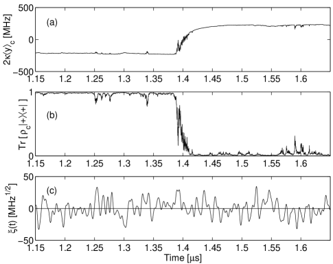
FIG. 3.: A close-up of the simulation in Fig. 2 showing (a) a switching event in the conditional mean of $y$, (b) the corresponding jump in atomic state, (c) the low-pass filtered noise sequence $\xi(t)$. Note the anomalous positively-biased part of the sequence (with a ‘spike’ at $t\approx 1.39$) that caused the jump.

In order to understand this ‘conspiracy’ we attempt to solve the simplified master equation (8) with the homodyne measurement term (9) added. We use the following ansatz for the coupled atom–field state

$$\rho=\sum_{a=\pm}|{a}\rangle\langle{a}|\otimes\int dy\,P_{a}(y)|{\bar{\alpha}+iy/2}\rangle\langle{\bar{\alpha}+iy/2}|,$$ (11)

where the field states are coherent states, so that $P(y)$ is really the Glauber-Sudarshan $P(\alpha)$ function on a line. Substituting this into Eq. (8) yields

$$\dot{P}_{\pm}(y) = \left[\frac{\partial}{\partial{y}}(\pm g+\kappa y)+\sqrt{2\kappa\eta}\,\xi(t)(y-\langle{y}\rangle)\right]P_{\pm}(y)$$ (13)

$$+\,(\gamma_{\perp}/2)\left[-P_{\pm}(y)+P_{\mp}(y)\right].$$

There is an implicit coupling between the two distributions in the measurement terms because

$$\langle{y}\rangle=\sum_{a=\pm}\int dy\,yP_{a}(y)=\sum_{a=\pm}p_{a}\langle{y}\rangle_{a},$$ (14)

where $p_{a}=\int dy\,P_{a}(y)={\rm Tr}[\rho|{a}\rangle\langle{a}|]$.

The effect of the first term in Eq. (13) is to drive the field towards the semiclassical fixed point $y^{\rm fix}_{\pm}=\mp g/\kappa$, as in Eq. (5). The second (measurement) term tries to localize the distribution at the current mean $\langle{y}\rangle$. The final (spontaneous emission) term drives the system towards an equal mixture of the two atomic states by locally transferring probability between $P_{+}$ and $P_{-}$ at each point $y$. It is the tension between these three processes (correlation of atomic state with field phase, localization of the field phase, and destruction of correlations) which gives rise to the discrete switching events between

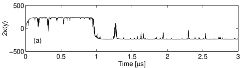
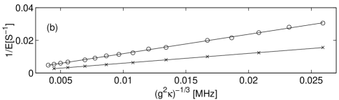
FIG. 4.: (a) Simulation of the simplified equation Eq. (13) with parameters as in Fig. 2, (b) scaling of $1/{\rm E}[1/S]$ with $g/\kappa$ fixed ($\eta=1$, $\gamma_{\perp}=1.3$ MHz for $\circ$’s and $0.65$ MHz for $\times$’s).

bistable fixed points. The dynamics of Eq. (13) is simulated in Fig. 4 with the same parameter values used with the full SME. Note that these simulations were computationally far less demanding than those of the full SME. The plots in the figure could easily be generated on a PC [13]. We find little difference between the simulated photocurrents of Eq. (13) and the full SME [14].

We can now use the simplified dynamics of Eq. (13) to understand how homodyne detection can cause quantum jumps. The probability for the atom to be in the upper state $|{+}\rangle$ is $p_{+}=\int dy\,P_{+}(y).$ From Eq. (13) this obeys

$$\dot{p}_{+}=\sqrt{2\kappa\eta}\,\xi(t)(p_{+}-p_{+}^{2})\Delta_{y}-\gamma_{\perp}(p_{+}-\mbox{$\frac{1}{2}$}),$$ (15)

where $\Delta_{y}\equiv\langle{y}\rangle_{+}-\langle{y}\rangle_{-}$. Consider the initial condition $|{\psi}\rangle=|{\psi_{+}^{\rm fix}}\rangle$. The damping of the atom (which drives $p_{+}$ towards its unconditioned equilibrium value of $\frac{1}{2}$) immediately produces a small component $p_{-}$. The field associated with this component will drift towards positive values of $y$. Thus $\Delta_{y}$ is negative. Say $\xi(t)$ then happens to be generally greater than zero over some short time interval. Since $0\leq p_{u}\leq 1$, it follows that $p_{+}-p_{+}^{2}\geq 0$. Thus the effect of a positive $\xi(t)$ on $p_{+}$ is to decrease it by transferring population to state $|{-}\rangle$.

This implication of Eq. (15) may be understood as follows. A sustained positive trend in $\xi(t)$ indicates a significant positive photocurrent fluctuation, such as could also take place if the $y$ quadrature of the field were actually increasing. Such an increase in $y$ could be caused by a quantum jump of the atom into the $|{-}\rangle$ state, but would otherwise be unlikely to occur. The stochastic master equation agrees with this line of reasoning, but reverses the causality so that occasional randomly-occurring biases in the photocurrent noise $\xi(t)$ actually cause the atom to change its state, as if the jumps are induced retroactively to justify the atypical photocurrent fluctuations. Returning to our example, note that if $\xi(t)$ tends to stay below zero (or fluctuates symmetrically about zero) then $p_{-}$ will be suppressed, $y$ will stay closed to the fixed point, and the atom will not have any ‘reason’ to change its state. This mechanism for the generation of ‘retroactive’ quantum jumps is confirmed by simulations of the full SME, as in Fig. 3.

A quantitative test of our analysis can be made by considering the non-negative entropy-like variable

$$S=p_{+}-p_{+}^{2},$$ (16)

which is zero when the atom is in a pure state and $\frac{1}{4}$ when it is in a completely mixed state. From Eq. (15) we can derive the following using Itô calculus

$$\frac{\partial}{\partial{t}}{\rm E}[\log S]=\kappa\eta{\rm E}\left[(2S-1)\Delta_{y}^{2}\right]+\gamma_{\perp}{\rm E}\left[\frac{1-4S}{2S}\right].$$ (17)

Here E denotes expectation value with respect to the stochasticity in the measurement term (9), as opposed to the quantum expectation values which are denoted as, for example, $\langle{y}\rangle_{+}$. Now since we expect $S$ to be generally small we can ignore it compared to unity. Taking the stationary solution of this equation then gives

$$\gamma_{\perp}{\rm E}[1/(2S)]=\kappa\eta{\rm E}[\Delta_{y}^{2}].$$ (18)

To estimate ${\rm E}[\Delta_{y}^{2}]$ we use the fact that the system stays close to $|{\psi_{\pm}^{\rm fix}}\rangle$ most of the time. Suppose it starts in state $|{\psi_{+}^{\rm fix}}\rangle$ so that $y_{+}=y_{+}^{\rm fix}=-g/\kappa$. Then the spontaneous emission generates probability at a rate $\gamma_{\perp}/2$ for the atom to be in the state $|{-}\rangle$. The associated field $y_{-}$ will drift towards $y_{-}^{\rm fix}$ and for short times $t\ll\kappa$ can be approximated by $y_{-}(t)=-g/\kappa+2gt$. This will persist only until the photocurrent signal it would have generated can be distinguished reliably from the photocurrent signal generated by the field $y_{+}=y_{+}^{\rm fix}$. The integrated difference between the two signals over a time $\tau$ is, from Eq. (10), $\kappa\eta g\tau^{2}$. The rms-noise in the signal is, again from Eq. (10), $\sqrt{\kappa\eta\tau}$. According to our explanation for the retroactive quantum jumps, the atom must decide which state to be in at the time $\tau$ such that the signal and noise are comparable, $\tau\sim(\kappa\eta g^{2})^{-1/3}$. It will then (most likely) decide to remain in state $|{+}\rangle$, and the process ‘repeats’ (it is actually continuous). The average of $(y_{+}-y_{-})^{2}$ up to time $\tau$ is easily evaluated to be $\sim(g/\kappa\eta)^{2/3}$. Substituting this into Eq. (18) gives

$$\frac{1}{{\rm E}[S^{-1}]}\sim\frac{\gamma_{\perp}}{2g^{2/3}(\kappa\eta)^{1/3}}.$$ (19)

This formula is valid for $g\eta^{1/2}\gtrsim\kappa$ and $\gamma_{\perp}\ll g^{2/3}(\kappa\eta)^{1/3}$.

The scaling of $1/{\rm E}[1/S]$ with the dynamical parameters of the system was tested using simulations of Eq. (13). The results, shown in Fig. 3b, are in excellent agreement with the prediction within its regime of validity. It is interesting that the atomic entropy $\sim 1/{\rm E}[S^{-1}]$ increases very slowly ($\sim\eta^{-1/3}$) with decreasing homodyne detection efficiency $\eta$. By contrast, detecting the atom’s fluorescence as in Ref. [10] would give an entropy $\sim 1-\eta$.

These results demonstrate that we do understand how the ‘quantum diffusion’ caused by homodyne monitoring of the cavity can induce ‘quantum jumps’ of the (unmonitored) atom. It should be noted that the master equation for radiative decay does not imply that the atom has any intrinsic preference to undergo jump-like behavior. As discussed in Ref. [15] for example, homodyne monitoring of the atom’s fluorescence would cause it to undergo diffusive evolution. The atomic jumps we have investigated above are truly a dynamical consequence of the strong correlation between the atomic state and the phase of the intracavity field, which itself stems from the Jaynes-Cummings Hamiltonian. There is no reason to believe that retroactive quantum jumps are unique to this particular system. We expect that using the stochastic master equation technique to investigate partially-observed strongly-coupled quantum systems will turn up many other examples of this new phenomenon.

H. M. would like to acknowledge the Advanced Computing Laboratory of LANL. H.M.W. was supported by the Australian Research Council.

REFERENCES

- [1] H. J. Carmichael, An Open Systems Approach to Quantum Optics (Springer, Berlin 1993).
- [2] H.M. Wiseman and G.J. Milburn, Phys. Rev. A 47, 642 (1993).
- [3] R. Dum et al, Phys. Rev. A 46, 4382 (1992).
- [4] J. Dalibard, Y. Castin, and K. Mølmer, Phys. Rev. Lett. 68, 580 (1992).
- [5] C.W. Gardiner, Handbook of Stochastic Methods (Springer, Berlin, 1985).
- [6] E. T. Jaynes and E. Cummings, Proc. IEEE 51, 89 (1963).
- [7] H. J. Kimble, in Cavity Quantum Electrodynamics, ed. P. Berman (Academic, San Diego 1994).
- [8] H. Mabuchi et al, Opt. Lett. 21, 1393 (1996).
- [9] C. J. Hood et al, Phys. Rev. Lett. 80, 4157 (1998).
- [10] P. Alsing and H. J. Carmichael, Quantum Opt. 3, 13 (1991).
- [11] In order to improve the strong convergence of the numerical integration, we used a semi-implicit Milstein strategy [12]. We used a truncated cavity basis of Fock states.
- [12] P. D. Drummond and I. K. Mortimer, Comput. Phys. 93, 144 (1991); P. E. Kloeden, E. Platen, and H. Schurz, Numerical Solution of SDE Through Computer Experiments, (Springer, Berlin 1994).
- [13] We integrated the -function evolution on a grid of 128 points. Care was required in the placing of grid points and the discretization of derivatives because of the pathological absence of diffusive terms in equation Eq. (13).
- [14] Differences that do exist may be due to the fact that the parameters chosen do not satisfy the condition .
- [15] H.M. Wiseman and G.J. Milburn, Phys. Rev. A 47, 1652 (1993).