Absorption with inversion and amplification without inversion in a coherently prepared V - system: a dressed state approach

Abstract

Light induced absorption with population inversion and amplification without population inversion (LWI) in a coherently prepared closed three level V - type system are investigated. This study is performed from the point of view of a two color dressed state basis. Both of these processes are possible due to atomic coherence and quantum interference contrary to simple intuitive predictions. Merely on physical basis, one would expect a complementary process to the amplification without inversion. We believe that absorption in the presence of population inversion found in the dressed state picture utilized in this study, constitutes such a process.

Novel approximate analytic time dependent solutions, for coherences and populations are obtained, and are compared with full numerical solutions exhibiting excellent agreement. Steady state quantities are also calculated, and the conditions under which the system exhibits absorption and gain with and without inversion, in the dressed state representation are derived. It is found that for a weak probe laser field absorption with inversion and amplification without inversion may occur, for a range of system parameters.

*shuker@bgumail.bgu.ac.il

I Introduction

Recently there has been tremendous interest in the study of light amplification and lasing without the requirement of population inversion (LWI), potentially capable of extending the range of laser devices to spectral region in which, for various reasons, population inversion is difficult to achieve. These spectral regions include UV which can be obtained from atomic vapor, and mid-to-far infrared, obtained by interssubband transitions in quantum wells. Many models for LWI have been proposed, mostly three and four level schemes, in $\Lambda$ and $V$ configurations. The dependence of optical gain on system parameters has also been investigated [1, 2, 3, 4, 5, 6, 7, 8, 9, 10, 11, 12, 13, 14, 15, 16, 17].
The key mechanism, which is common to most of the proposed schemes, is the utilization of external coherent fields, that induce quantum coherence and interference in multilevel systems. An exception of LWI without the use of coherent fields was also reported [9]. In particular it was shown that if atomic coherence between certain atomic states is established , different absorption processes may interfere destructively leading to the reduction or even the cancellation of absorption [7, 13]. At the same time stimulated emission may remain intact, leading to the possibility of gain even if only a small fraction of the population is in the excited state.
Experimental observations of inversionless gain and lasing without inversion have been reported by several groups [18, 19, 20, 21]. Inversionless lasers have been shown to have unique properties such as non classical photon statistics and substantially narrow spectral features [22, 23]. In a recent paper, Y. Zhu [12] analyzed the transient and steady state properties of light amplification without population inversion in a closed three level V type system in the bare state basis. Steady state dressed state populations were also calculated, in the limit of strong driving laser.

In this paper we study a V- type three level model within the framework of the dressed state basis, and give explicit analytic time dependent solutions, as well as steady state solutions for populations and coherences. This paper details the calculations of LWI in the dressed state basis, which is valid to some extent for atoms dressed both by the pump and probe lasers. More over we offer a set of theoretical tools allowing one to obtain explicit time dependent solutions for populations and coherences. These calculations show the possibility of inversion and inversionless gain in the dressed basis as well as gain without population inversion in the bare state representation. A novel interesting feature found in this study is the existence of absorption despite population inversion. Although this effect is contrary to simple physical intuitive explanation of absorption, this process has a conceptual reasoning. From basic physical arguments one expects a complementary process to amplification without inversion. We believe that absorption in the presence of population inversion, found in the dressed state picture, constitutes such a process. It is another manifestation of the quantum interference that may occur in multilevel systems where coherently prepared states present the possibility of interfering channels [24]. This phenomenon should be interpreted as a quantum interference constructive process for the stimulated absorption just as LWI is obtained from a quantum interference destructive process of absorption.

In Sec. II we present the model system and the master equation used to derive the equations of motion for the elements of the density matrix. We have chosen to employ a fully quantum mechanical Hamiltonian, even though later on the density matrix equations are reduced to their semiclassical version. The quantum mechanical Hamiltonian gives rise to a simple picture of the stationary dressed states. In Sec. III the dressed levels are introduced and the master equation is projected over the dressed state basis. Physical interpretation of relaxation coefficients in the dressed basis is given and the role that quantum coherences and interferences play is elucidated. In Sec. IV we present time dependent and steady state solutions for the dressed state populations and coherences. Comparison is made with the bare state results.

II Hamiltonian and master equation for the atom

Let us consider the closed V-type three level system illustrated in figure 1. The transition $|a>\leftrightarrow|b>$ of frequency $\omega_{ba}$ is driven by a strong single mode laser of frequency $\omega_{L}$ . The transition $|a>\leftrightarrow|c>$ of frequency $\omega_{ca}$ is pumped incoherently with a rate $\Lambda$. A single mode probe laser(not necessarily weak) is applied to the transition $|a>\leftrightarrow|c>$. $\gamma_{b}$ ($\gamma_{c}$ ) is the spontaneous emission rate from the state $|b>$ ($|c>$). The states $|b>$ and $|c>$ are not directly coupled.

We have chosen to work within the frame of the master equation for the atom, since it being an operator equation independent of representation, it can be projected over any basis. We use a generalization of a standard master equation adjusted to account for the scheme described above [25]. The master equation is given by:

$$\dot{\sigma} = -\frac{i}{\hbar}[H,\sigma]-\frac{\gamma_{b}}{2}[s_{+}s_{-}\sigma+\sigma s_{+}s_{-}]+\gamma_{b}s_{-}\sigma s_{+}-\frac{\gamma_{c}}{2}[s^{\prime}_{+}s^{\prime}_{-}\sigma+\sigma s^{\prime}_{+}s^{\prime}_{-}]+\gamma_{c}s^{\prime}_{-}\sigma s^{\prime}_{+}$$ (2)

$$\mbox{}-\frac{\Lambda}{2}[s^{\prime}_{+}s^{\prime}_{-}\sigma+\sigma s^{\prime}_{+}s^{\prime}_{-}]-\frac{\Lambda}{2}[s^{\prime}_{-}s^{\prime}_{+}\sigma+\sigma s^{\prime}_{-}s^{\prime}_{+}]+\Lambda s^{\prime}_{+}\sigma s^{\prime}_{-}+\Lambda s^{\prime}_{-}\sigma s^{\prime}_{+},$$

here $\sigma$ is the density operator for the atom. $s_{+}(s_{-})$, $s^{\prime}_{+}(s^{\prime}_{-})$ are the atomic raising and lowering operators, for the $|a>\leftrightarrow|b>$ and $|a>\leftrightarrow|c>$ transitions respectively. H is the Hamiltonian of the global system and we take it to be fully quantum mechanical. The quantum mechanical Hamiltonian gives rise to a simple picture of the stationary dressed states. The Hamiltonian in the dipole and rotating wave approximation is given by:

$$H = \hbar\omega_{ba}|b><b|+\hbar\omega_{ca}|c><c|+\hbar\omega_{L}(a^{\dagger}a+\frac{1}{2})+\hbar\omega_{p}(a^{\prime\dagger}a^{\prime}+\frac{1}{2})$$ (4)

$$\mbox{}+g(s_{+}a+s_{-}a^{\dagger})+g^{\prime}(s^{\prime}_{+}a^{\prime}+s^{\prime}_{-}a^{\prime\dagger}).$$

$g$ and $g^{\prime}$ are coupling constants and are assumed to be real. The eigenstates of the unperturbed part of the Hamiltonian form a three dimensional manifold labeled  by the atomic indexes, the laser photon number $N$ and by the probe photon number $N^{\prime}$. The manifold is written

$$\varepsilon(N,N^{\prime})=\{|a,N+1,N^{\prime}+1>,|b,N,N^{\prime}+1>,|c,N+1,N^{\prime}>\}.$$ (5)

We represent the uncoupled eigenstates of the atom and the two non-interacting field modes as:

$$|a,N+1,N^{\prime}+1>=\left(\begin{array}[]{c}1\\ 0\\ 0\end{array}\right)\hskip 10.84006pt|b,N,N^{\prime}+1>=\left(\begin{array}[]{c}0\\ 1\\ 0\end{array}\right)\hskip 10.84006pt|c,N+1,N^{\prime}>=\left(\begin{array}[]{c}0\\ 0\\ 1\end{array}\right).$$ (6)

In this basis the hamiltonian takes the form

$$H_{Int}=\left(\begin{array}[]{ccc}0&-\Omega&-G\\ -\Omega&-\Delta_{1}&0\\ -G&0&-\Delta_{2}\end{array}\right).$$ (7)

Where we have defined the Rabi frequencies and the detunigs, in their quantum form by

$$-g\sqrt{N+1}=\hbar\Omega\hskip 7.22743pt;\hskip 7.22743pt-g^{\prime}\sqrt{N^{\prime}+1}=\hbar G\hskip 7.22743pt;\hskip 7.22743pt\Delta_{1}=\omega_{L}-\omega_{ba}\hskip 7.22743pt;\hskip 7.22743pt\Delta_{2}=\omega_{p}-\omega_{ca}.$$ (8)

To obtain the semiclassical equations of motion for the elements of the density matrix we project the master equation (2) over the basis (6) and perform the following reduction operation by introducing the reduced populations and coherences $\rho_{ij}$ via:

$$\rho_{aa} = \sum_{N,N^{\prime}}<a,N+1,N^{\prime}+1|\sigma|a,N+1,N^{\prime}+1>,$$ (10)

$$\rho_{ab} = \sum_{N,N^{\prime}}<a,N+1,N^{\prime}+1|\sigma|b,N,N^{\prime}+1>.$$ (11)

and similar relations for the other populations and coherences. Taking into account the above reduced quantities we obtain the density matrix equations

$$\dot{\rho}_{aa} = -\Lambda\rho_{aa}+(\Lambda+\gamma_{c})\rho_{cc}+\gamma_{b}\rho_{bb}+i\Omega(\rho_{ba}-\rho_{ab})+iG(\rho_{ca}-\rho_{ac}),$$ (13)

$$\dot{\rho}_{bb} = -\gamma_{b}\rho_{bb}+i\Omega(\rho_{ab}-\rho_{ba}),$$ (14)

$$\dot{\rho}_{cc} = \Lambda\rho_{aa}-(\Lambda+\gamma_{c})\rho_{cc}+iG(\rho_{ac}-\rho_{ca}),$$ (15)

$$\dot{\rho}_{ab} = -[\frac{1}{2}(\Lambda+\gamma_{b})+i\Delta_{1}]\rho_{ab}+i\Omega(\rho_{bb}-\rho_{aa})+iG\rho_{cb},$$ (16)

$$\dot{\rho}_{ac} = -[\frac{1}{2}(\Lambda+\gamma_{c})+i\Delta_{2}]\rho_{ac}+iG(\rho_{cc}-\rho_{aa})+i\Omega\rho_{bc},$$ (17)

$$\dot{\rho}_{bc} = -[\frac{1}{2}(\Lambda+\gamma_{b}+\gamma_{c})+i(\Delta_{2}-\Delta_{1})]\rho_{bc}+i\Omega\rho_{ac}-iG\rho_{ba}.$$ (18)

III Dressed states and density matrix equations in the dressed state basis

The dressed states are obtained by finding the the eigenvectors of the interaction Hamiltonian, Eq. (7). To simplify things a little we take both the driving laser field and the probe field to be in exact resonance with the corresponding bare state transitions, i.e., we take $\Delta_{1}=~{}\Delta_{2}=0$. When the detunings are set to zero we notice that the energies in the bare state basis are all degenerate, and in fact equal to zero (in the interaction picture). Carrying out the diagonalization procedure we obtain the following eigenstates:

$$|\alpha(N)(N^{\prime})> = -\frac{G}{R}\hskip 2.84544pt|b,N,N^{\prime}+1>+\frac{\Omega}{R}\hskip 2.84544pt|c,N+1,N^{\prime}>,$$ (20)

$$|\beta(N)(N^{\prime})> = -\frac{1}{\sqrt{2}}\hskip 2.84544pt|a,N+1,N^{\prime}+1>+\frac{\Omega}{\sqrt{2}R}\hskip 2.84544pt|b,N,N^{\prime}+1>+\frac{G}{\sqrt{2}R}\hskip 2.84544pt|c,N+1,N^{\prime}>,$$ (21)

$$|\gamma(N)(N^{\prime})> = \frac{1}{\sqrt{2}}\hskip 2.84544pt|a,N+1,N^{\prime}+1>+\frac{\Omega}{\sqrt{2}R}\hskip 2.84544pt|b,N,N^{\prime}+1>+\frac{G}{\sqrt{2}R}\hskip 2.84544pt|c,N+1,N^{\prime}>.$$ (22)

and the corresponding energies

$$E_{|\gamma>}=-\hbar R\hskip 36.135pt;\hskip 36.135ptE_{|\alpha>}=0\hskip 36.135pt;\hskip 36.135ptE_{|\beta>}=\hbar R.$$ (23)

Where we have introduced the on resonance, two field generalized Rabi flopping frequency $R=\sqrt{\Omega^{2}+G^{2}}$.

Note that for the case $G=0$ equations (21) and (22) render the usual coupling and non coupling dressed states, while the $|\alpha>$ state which is identical to the $|c>$ state is not involved in the interaction altogether. The energy ladder is shown schematically in figure 2. We can see that one state remained intact, while the other two states were displaced by an energy amount of $\hbar R$, with respect to the bare states. In the strong driving field limit, i.e., when $\Omega>>~{}G$, we see that the $|\alpha(N)(N^{\prime})>$ state has the character of the excited bare state $|c,N+1,N^{\prime}>$ and hence is expected to be less populated than the other two states. By contrast, the $|\beta(N)(N^{\prime})>$ and $|\gamma(N)(N^{\prime})>$ states have a ground state character, and hence will be more populated than the $|\alpha(N)(N^{\prime})>$ state. However both $|\beta>$ and $|\gamma>$ states are also contaminated by the same amount of the first excited level and thus they are expected to possess the same population content.

The eigenstates of equations (20)-(22) define a rotation matrix (transformation matrix)

$$T=\left(\begin{array}[]{ccc}0&-\frac{G}{R}&\frac{\Omega}{R}\\ \\ -\frac{1}{\sqrt{2}}&\frac{\Omega}{\sqrt{2}R}&\frac{G}{\sqrt{2}R}\\ \\ \frac{1}{\sqrt{2}}&\frac{\Omega}{\sqrt{2}R}&\frac{G}{\sqrt{2}R}\end{array}\right)$$ (24)

that diagonalizes the Hamiltonian of Eq.(7) via the matrix product $THT^{-1}$. Thus the density operator in the dressed atom basis, $\rho^{Dr}$, will be given by the matrix product

$$\rho^{Dr}=T\rho^{B}T^{-1}$$ (25)

where $\rho^{B}$ is the density operator in the bare basis.

Projection of the master equation over the dressed state basis yields particularly simple equations for the first part of Eq.(2), i.e., the Hamiltonian part of the master equation. However, in the dressed atom basis the relaxation terms of Eq.(2) give rise to equations that are not as simple as equations (13-18). In particular couplings between dressed state populations and coherences between two dressed states appear. In the next section we present an approximate version of the complete set of equations given bellow.

The equation of motion for the density matrix elements in the dressed state representation are given by:

$$\dot{\rho}_{\alpha\alpha} = -(\Gamma_{\alpha}+\Lambda^{\prime})\rho_{\alpha\alpha}+\tilde{\Gamma}(\rho_{\alpha\beta}+\rho_{\beta\alpha})+\tilde{\Gamma}(\rho_{\alpha\gamma}+\rho_{\gamma\alpha})+\frac{1}{2}\Lambda^{\prime}\rho_{\beta\beta}$$ (28)

$$\mbox{}-\frac{1}{2}\Lambda^{\prime}(\rho_{\beta\gamma}+\rho_{\gamma\beta})+\frac{1}{2}\Lambda^{\prime}\rho_{\gamma\gamma}$$

$$\dot{\rho}_{\alpha\beta} = -(\Gamma_{\alpha\beta}-iR)\rho_{\alpha\beta}-(\Gamma_{\beta}-\frac{1}{4}\Lambda^{\prime})\rho_{\alpha\gamma}-\tilde{\Gamma^{\prime}}\rho_{\beta\gamma}+(\tilde{\Gamma}-\tilde{\Gamma^{\prime}})\rho_{\gamma\beta}$$ (30)

$$\mbox{}+\tilde{\Gamma}\rho_{\alpha\alpha}+(\tilde{\Gamma}+\tilde{\Gamma^{\prime}})\rho_{\beta\beta}+\tilde{\Gamma^{\prime}}\rho_{\gamma\gamma},$$

$$\dot{\rho}_{\alpha\gamma} = -(\Gamma_{\alpha\beta}+iR)\rho_{\alpha\gamma}-(\Gamma_{\beta}-\frac{1}{4}\Lambda^{\prime})\rho_{\alpha\beta}+(\tilde{\Gamma}-\tilde{\Gamma^{\prime}})\rho_{\beta\gamma}-\tilde{\Gamma^{\prime}}\rho_{\gamma\beta}$$ (32)

$$\mbox{}+\tilde{\Gamma}\rho_{\alpha\alpha}+\tilde{\Gamma^{\prime}}\rho_{\beta\beta}+(\tilde{\Gamma}+\tilde{\Gamma^{\prime}})\rho_{\gamma\gamma}$$

$$\dot{\rho}_{\beta\beta} = -(\Gamma_{\beta}+\frac{1}{2}\Lambda)\rho_{\beta\beta}+\frac{1}{2}(\Gamma_{\alpha}+\Lambda^{\prime})\rho_{\alpha\alpha}+(\Gamma_{\beta}+\frac{1}{2}\Lambda-\frac{1}{2}\Lambda^{\prime})\rho_{\gamma\gamma}$$ (34)

$$\mbox{}-\tilde{\Gamma}(\rho_{\alpha\gamma}+\rho_{\gamma\alpha})+\frac{1}{4}\Lambda^{\prime}(\rho_{\beta\gamma}+\rho_{\gamma\beta}),$$

$$\dot{\rho}_{\beta\gamma} = -(\Gamma_{\beta\gamma}+2iR)\rho_{\beta\gamma}-(\Gamma_{\beta}+\frac{1}{2}\Lambda-\frac{1}{2}\Lambda^{\prime})\rho_{\gamma\beta}+\tilde{\Gamma}(\rho_{\alpha\beta}+\rho_{\gamma\alpha})$$ (36)

$$\mbox{}+2\tilde{\Gamma}(\rho_{\beta\alpha}+\rho_{\alpha\gamma})-\frac{1}{2}(\Gamma_{\alpha}+\Lambda^{\prime})\rho_{\alpha\alpha}-(2\Gamma_{\beta}-\frac{1}{4}\Lambda^{\prime})(\rho_{\beta\beta}+\rho_{\gamma\gamma})$$

$$\dot{\rho}_{\gamma\gamma} = -(\Gamma_{\beta}+\frac{1}{2}\Lambda)\rho_{\gamma\gamma}-\tilde{\Gamma}(\rho_{\alpha\beta}+\rho_{\beta\alpha})+\frac{1}{4}\Lambda^{\prime}(\rho_{\beta\gamma}+\rho_{\gamma\beta})$$ (38)

$$\mbox{}+\frac{1}{2}(\Gamma_{\alpha}+\Lambda^{\prime})\rho_{\alpha\alpha}+(\Gamma_{\beta}+\frac{1}{2}\Lambda-\frac{1}{2}\Lambda^{\prime})\rho_{\beta\beta}$$

Where we have again made use of the reduction operation

$$\rho_{i,j}=\sum_{N,N^{\prime}}<i(N)(N^{\prime})|\sigma|j(N)(N^{\prime})>\hskip 28.45274pti,j=|\alpha>,|\beta>,|\gamma>$$ (39)

In obtaining equations (28) - (38) we have introduced the following notation

$$\Gamma_{\alpha} = \frac{1}{R^{2}}(\gamma_{b}G^{2}+\gamma_{c}\Omega^{2})\hskip 5.69046pt,\hskip 5.69046pt\Gamma_{\beta}=\frac{1}{4R^{2}}(\gamma_{b}\Omega^{2}+\gamma_{c}G^{2})\hskip 5.69046pt,$$

$$\Gamma_{\alpha\beta} = \Gamma_{\beta}+\frac{1}{2}(\Gamma_{\alpha}+\Lambda+\Lambda^{\prime}/2)\hskip 5.69046pt,\hskip 5.69046pt\Gamma_{\beta\gamma}=3\Gamma_{\beta}+\frac{3}{2}\Lambda-\Lambda^{\prime},$$

$$\tilde{\Gamma} = \frac{G\Omega}{2\sqrt{2}R^{2}}(\gamma_{b}-\gamma_{c}-\Lambda)\hskip 5.69046pt,\hskip 5.69046pt\tilde{\Gamma^{\prime}}=\frac{G\Omega\Lambda}{2\sqrt{2}R^{2}}\hskip 5.69046pt,\hskip 5.69046pt\Lambda^{\prime}=\frac{\Lambda\Omega^{2}}{R^{2}}.$$

$\Gamma_{\alpha}$, $\Gamma_{\beta}$ are the spontaneous emission decay rate of the $|\alpha>$, $|\beta>$ and $|\gamma>$ states ($|\gamma>$ also decays with a rate $\Gamma_{\beta}$). More precisely the state $|\alpha(N)(N^{\prime})>$ decays by spontaneous emission with a rate $\Gamma_{\alpha}$ to the levels $|\beta(N-1)(N^{\prime})>$, $|\gamma(N-1)(N^{\prime})>$ , $|\beta(N)(N^{\prime}-1)>$ and $|\gamma(N)(N^{\prime}-1)>$. Similarly the levels $|\beta(N)(N^{\prime})>$, $|\gamma(N)(N^{\prime})>$ decay with the same rate $\Gamma_{\beta}$ to the same levels as $|\alpha(N)(N^{\prime})>$. The coherences $\rho_{\alpha\beta}$, and $\rho_{\alpha\gamma}$ ($\rho_{\beta\gamma}$) decay with a rate $\Gamma_{\alpha\beta}$ ($\Gamma_{\beta\gamma}$). $\Lambda^{\prime}$ is a dressed picture pump rate which causes population and depopulation of the dressed levels. It also has an important influence on the coherences as can readily be seen from Eqs. (28) - (38). $\tilde{\Gamma}$ and $\tilde{\Gamma^{\prime}}$ are identified as interference terms. They involve the product of two Rabi frequencies. Both parameters vanish whenever either $G$ or $\Omega$ are zero. These terms are responsible for the amplification without inversion and for the absorption despite the inversion. This fact is verified numerically. When we have set both $\tilde{\Gamma}$ and $\tilde{\Gamma^{\prime}}$ zero (this happens when $\Lambda=0$ and $\gamma_{b}=\gamma_{c}$) any previously obtained gain has vanished. The first and second terms in $\Gamma_{\alpha\beta}$ describe damping of the atomic coherence due to radiative transitions of the levels involved to lower levels, and is equal to half the sum of all transition rates starting from $|\alpha(N)(N^{\prime})>$ and $|\beta(N)(N^{\prime})>$. The third term in $\Gamma_{\alpha\beta}$ describes coherence damping due to the incoherent pump. The interpretation of $\Gamma_{\beta\gamma}$ is similar except that the $3\Gamma_{\beta}$ is composed of a $2\Gamma_{\beta}$ term responsible for the coherence damping due to radiative transition, plus a single $\Gamma_{\beta}$ component resulting from transfer of coherence from higher levels belonging to higher manifolds. This fact would have been transparent had we written the non reduced version of Eqs. ( 28) - (38). Inspection of equations (13) reveals that $\rho_{\alpha\beta}$ and $\rho_{\alpha\gamma}$ have the same free frequency R, however they oscillate out of phase. The free evolution frequency of $\rho_{\beta\gamma}$ is twice as large, as both levels $|\beta>$ and $|\gamma>$ are contaminated by the bare ground state $|a>$. Note that the closure of the system is satisfied by Eq.(28)-(38), i.e., $\frac{d}{dt}(\rho_{\alpha\alpha}+\rho_{\beta\beta}+\rho_{\gamma\gamma})=0$. Gain or absorption coefficient for the $|j>\rightarrow|i>$ transition is proportional to $Im[\rho_{ij}]$. In our notation amplification will occur if $Im[\rho_{ij}]>0$.
In the next section we present approximate solutions of Eq.s (28)-(38), both the temporal and the steady state cases. These will be compared with numerical calculations of the full system, i.e., without any approximation.

IV Density matrix equations in the dressed state basis in the secular approximation

As mentioned before the Hamiltonian part of the master equation has a simple form in the dressed state basis given by Eqs. (20-22) (the Hamiltonian is diagonalized in the dressed state representation). The problem arises when the spontaneous emission and pump terms are present in the master equation,Eq.(2), giving the complicated couplings appearing in equations (28) - (38). Solving exactly the complete set seems to be a formidable task even with “Mathematica” [26]. However, the situation can be simplified if the frequency difference between the dressed states of the manifold, namely the Rabi flopping frequency $R$ is large compared with the rates $\gamma_{b}$, $\gamma_{c}$ ,$\Lambda$. We can then ignore the “nonsecular” terms, i.e., couplings between populations and coherences (see [25]).

a The evolution of the population terms.

When the “nonsecular” couplings between populations and coherences are ignored we obtain from (28), (34) and (38) the following equations for the populations:

$$\dot{\rho}_{\alpha\alpha} = -(\Gamma_{\alpha}+\Lambda^{\prime})\rho_{\alpha\alpha}+\frac{1}{2}\Lambda^{\prime}\rho_{\beta\beta}+\frac{1}{2}\Lambda^{\prime}\rho_{\gamma\gamma},$$ (41)

$$\dot{\rho}_{\beta\beta} = -(\Gamma_{\beta}+\frac{1}{2}\Lambda)\rho_{\beta\beta}+\frac{1}{2}(\Gamma_{\alpha}+\Lambda^{\prime})\rho_{\alpha\alpha}+(\Gamma_{\beta}+\frac{1}{2}\Lambda-\frac{1}{2}\Lambda^{\prime})\rho_{\gamma\gamma},$$ (42)

$$\dot{\rho}_{\gamma\gamma} = -(\Gamma_{\beta}+\frac{1}{2}\Lambda)\rho_{\gamma\gamma}+\frac{1}{2}(\Gamma_{\alpha}+\Lambda^{\prime})\rho_{\alpha\alpha}+(\Gamma_{\beta}+\frac{1}{2}\Lambda-\frac{1}{2}\Lambda^{\prime})\rho_{\beta\beta}.$$ (43)

Note that population conservation is still maintained. The interpretation of equations (41)-(43) is very clear. The state $|\alpha>$ is depopulated with a rate $(\Gamma_{\alpha}+\Lambda^{\prime})$, which in turn, is distributed equally among the states $|\beta>$ and $|\gamma>$, as can be readily seen from the one half factor multiplying the coefficient of $\rho_{\alpha\alpha}$ in (42) and (43). The state $|\alpha>$ is also being populated with a rate $\frac{1}{2}\Lambda$ by the states $|\beta>$ and $|\gamma>$. The state $|\beta>$ ($|\gamma>$) is depopulated at a rate $(\Gamma_{\beta}+\frac{1}{2}\Lambda)$ and repopulated with the same rate from $|\gamma>$ ($|\beta>$). The set (41) -(43) can be solved exactly by calculating its eigenvalues and eigenstates, subject to the condition $\rho_{\alpha\alpha}+\rho_{\beta\beta}+\rho_{\gamma\gamma}=1$. This yields the temporal solution

$$\rho_{\alpha\alpha}(t) = \rho_{\alpha\alpha}^{st}+[\rho_{\alpha\alpha}(0)-\rho_{\alpha\alpha}^{st}]e^{-(\Gamma_{\alpha}+\frac{3}{2}\Lambda^{\prime})t},$$ (45)

$$\rho_{\beta\beta}(t) = \rho_{\beta\beta}^{st}+[\rho_{\beta\beta}(0)-\rho_{\beta\beta}^{st}+\frac{1}{2}(\rho_{\alpha\alpha}(0)-\rho_{\alpha\alpha}^{st})]e^{-(2\Gamma_{\beta}+\Lambda-\frac{1}{2}\Lambda^{\prime})t}$$ (46)

$$- \frac{1}{2}[\rho_{\alpha\alpha}(0)-\rho_{\alpha\alpha}^{st}]e^{-(\Gamma_{\alpha}+\frac{3}{2}\Lambda^{\prime})t},$$ (47)

$$\rho_{\gamma\gamma}(t) = \rho_{\gamma\gamma}^{st}-[\rho_{\beta\beta}(0)-\rho_{\beta\beta}^{st}+\frac{1}{2}(\rho_{\alpha\alpha}(0)-\rho_{\alpha\alpha}^{st})]e^{-(2{\Gamma_{\beta}}+\Lambda-\frac{1}{2}\Lambda^{\prime})t}$$ (48)

$$- \frac{1}{2}[\rho_{\alpha\alpha}(0)-\rho_{\alpha\alpha}^{st}]e^{-(\Gamma_{\alpha}+\frac{3}{2}\Lambda^{\prime})t}.$$ (49)

where $\rho_{ii}(0)$ are the initial populations. The steady state populations are given by

$$\rho_{\alpha\alpha}^{st} = \frac{\Lambda^{\prime}}{2\Gamma_{\alpha}+3\Lambda^{\prime}},$$ (51)

$$\rho_{\beta\beta}^{st}=\rho_{\gamma\gamma}^{st} = \frac{\Gamma_{\alpha}+\Lambda^{\prime}}{2\Gamma_{\alpha}+3\Lambda^{\prime}}.$$ (52)

We can see that the population $\rho_{\beta\beta}$, $\rho_{\gamma\gamma}$ have similar behavior, though not identical, a fact which is not surprising at all in light of the very similar composition of the states $|\beta>$ and $|\gamma>$. The population of the state $|\alpha>$ is unique in the sense that it decays with only one decay constant, while the other populations have a composite decay. Figure 3 shows a comparison between the exact solution for $\rho_{\alpha\alpha}$ and $\rho_{\beta\beta}$ (solid line), obtained by solving numerically the equation set (28) -(38), with our approximate analytic solution (45) - (49) shown in dashed line. The normalized parameters for the numerical simulation were set to be $\Omega=20\gamma_{c}$, $\gamma_{b}=2\gamma_{c}$, $G=0.1\gamma_{c}$, $\Lambda=3\gamma_{c}$. We can see that the population $\rho_{\alpha\alpha}$ is a monotonically increasing, oscillating function of time which reaches a steady state value $\rho_{\alpha\alpha}^{st}\approx 0.27$. The behavior of $\rho_{\beta\beta}$ is opposite, i.e., it is a monotonically decreasing oscillating function and it reaches the steady state value $\rho_{\beta\beta}^{st}\approx 0.36$. $\rho_{\gamma\gamma}$ is not shown because its similarity to $\rho_{\beta\beta}$, due the choice of parameters made. The approximate solutions describe nicely the envelope of oscillation and the correct expression for the steady state. One can see that $\rho_{\alpha\alpha}<\rho_{\beta\beta}=\rho_{\gamma\gamma}$, for any finite $\Lambda$, and hence population inversion do exist in the dressed state basis. For the transitions $|\alpha>\rightarrow|\beta>$, $|\alpha>\rightarrow|\gamma>$, $|\beta>\rightarrow|\gamma>$ and $|\gamma>\rightarrow|\beta>$ the population difference is negative (noninversion) and it remains to be seen whether this transitions amplify and thus result in lasing without inversion in the dressed state basis. In the strong coupling field limit, $\Omega>>G$ the steady state population become

$$\rho_{\beta\beta}=\rho_{\gamma\gamma}=\frac{\gamma_{c}+\Lambda}{2\gamma_{c}+3\Lambda},$$ (53)

and

$$\rho_{\alpha\alpha}=\frac{\Lambda}{2\gamma_{c}+3\Lambda}.$$ (54)

In the following we will get into more detail regarding gain without inversion in the dressed state basis.

b Evolution of coherences.

Ignoring the “non secular” couplings between coherences and populations in Eqs. (28) - (38) results in equations that are simpler than the original ones, however, they are still very complicated, particularly the equations for $\rho_{\beta\gamma}$ and it’s conjugate, which are coupled to all the other coherences. Hence one would like to further approximate these equations in such a way that the resulting solutions will be fairly simple on one hand, and be a reasonable approximation to the exact solution on the other. We solved numerically the complete set (28) -(38) and found that $\rho_{\beta\gamma}$ and hence its conjugate are substantially larger than the other coherences, indicating the crucial role these coherences play. In light of the above, we couple each atomic coherence to itself (describing the free evolution) and to $\rho_{\beta\gamma}$ and $\rho_{\gamma\beta}$ acting as the dominant source terms.

This gives the following equations:

$$\dot{\rho}_{\alpha\beta} = -(\Gamma_{\alpha\beta}-iR)\rho_{\alpha\beta}-\tilde{\Gamma^{\prime}}\rho_{\beta\gamma}+(\tilde{\Gamma}-\tilde{\Gamma^{\prime}})\rho_{\gamma\beta},$$ (56)

$$\dot{\rho}_{\alpha\gamma} = -(\Gamma_{\alpha\gamma}+iR)\rho_{\alpha\gamma}+(\tilde{\Gamma}-\tilde{\Gamma^{\prime}})\rho_{\beta\gamma}-\tilde{\Gamma^{\prime}}\rho_{\gamma\beta},$$ (57)

$$\dot{\rho}_{\beta\gamma} = -(\Gamma_{\beta\gamma}+2iR)\rho_{\beta\gamma}-(\Gamma_{\beta}+\frac{1}{2}\Lambda-\frac{1}{2}\Lambda^{\prime})\rho_{\gamma\beta},$$ (58)

along with the equation for $\rho_{\gamma\beta}=\rho_{\beta\gamma}^{*}$. Solving the eigenvalue problem of eq.’s (56) - (58) we find the transient solutions for the coherences , in the strong coupling field limit. These solutions are:

$$\rho_{\alpha\beta} = A\exp[-(\Gamma_{\alpha\beta}-iR)t]+C\frac{(\tilde{\Gamma}-\tilde{\Gamma^{\prime}})(\Gamma_{\beta}+\Lambda/2-\Lambda^{\prime}/2)+i4\tilde{\Gamma^{\prime}}R}{(\Gamma_{\beta}+\Lambda/2-\Lambda^{\prime}/2)(\Gamma_{\beta\gamma}-\Gamma_{\alpha\beta}+3iR)}\exp[-(\Gamma_{\beta\gamma}+2iR)t]$$ (60)

$$+ D\frac{(\tilde{\Gamma^{\prime}}-\tilde{\Gamma})+i\tilde{\Gamma^{\prime}}(\Gamma_{\beta}+\Lambda/2-\Lambda^{\prime}/2)/4R}{\Gamma_{\beta\gamma}-\Gamma_{\alpha\beta}-iR}\exp[-(\Gamma_{\beta\gamma}-2iR)t],$$ (61)

$$\rho_{\alpha\gamma} = B\exp[-(\Gamma_{\alpha\beta}+iR)t]+C\frac{\tilde{\Gamma^{\prime}}(\Gamma_{\beta}+\Lambda/2-\Lambda^{\prime}/2)-i4R(\tilde{\Gamma}-\tilde{\Gamma^{\prime}})}{(\Gamma_{\beta}+\Lambda/2-\Lambda^{\prime}/2)(\Gamma_{\beta\gamma}-\Gamma_{\alpha\beta}+iR)}\exp[-(\Gamma_{\beta\gamma}+2iR)t]$$ (62)

$$+ D\frac{\tilde{\Gamma^{\prime}}-i(\tilde{\Gamma}-\tilde{\Gamma^{\prime}})(\Gamma_{\beta}+\Lambda/2-\Lambda^{\prime}/2)/4R}{\Gamma_{\beta\gamma}-\Gamma_{\alpha\beta}-3iR}\exp[-(\Gamma_{\beta\gamma}-2iR)t],$$ (63)

$$\rho_{\beta\gamma} = C\frac{4iR}{\Gamma_{\beta}+\Lambda/2-\Lambda^{\prime}/2}\exp[-(\Gamma_{\beta\gamma}+2iR)t]+D\hskip 5.69046pti\hskip 5.69046pt\frac{\Gamma_{\beta}+\Lambda/2-\Lambda^{\prime}/2}{4R}\times$$ (64)

$$\times \exp[-(\Gamma_{\beta\gamma}-2iR)t],$$ (65)

where A, B, C and D are constants ought to be calculated from initial conditions. Figure 4 shows the exact coherences obtained by solving numerically eq.’s (28) -(38) (solid line), and the corresponding approximate solutions based on the analytic expressions (61) -(65). The chosen parameters are the same as in Fig 3. It can be seen that the exact solutions reach a steady state different from zero, while our approximate analytic solution have zero steady state values. This is due to the absence of the population source terms in the approximation. The oscillation frequency is predicted correctly by the approximate solutions. Moreover, the approximate solution for $\rho_{\beta\gamma}$ appears to be more accurate than the other two, again indicating the crucial role played by $\rho_{\beta\gamma}$ and $\rho_{\gamma\beta}$. Note also the negligible contribution of $\rho_{\alpha\beta}$ and $\rho_{\alpha\gamma}$ to $\rho_{\beta\gamma}$. The latter coherence is not coupled to $\rho_{\alpha\beta},\rho_{\alpha\gamma}$ yet the approximation remains satisfactory. Eq. (65) also shows that $\rho_{\beta\gamma}$ has an almost pure sinusoidal form of frequency $2R$. To the contrary $\rho_{\alpha\beta},\rho_{\alpha\beta}$ and $\rho_{\alpha\gamma}$ have a composite oscillation, being a superposition of frequencies. It can be seen from the numerical solution presented in figure 4 that the coherences $\rho_{\alpha\beta}$, and $\rho_{\alpha\gamma}$ possess a definite sign, thus the corresponding transitions between dressed states, being either amplified or attenuated. More precisely $Im(\rho_{\alpha\beta})$ is positive in all the range shown, hence the transition $|\beta>\rightarrow|\alpha>$ is amplified (with population inversion in the dressed state picture at the frequencies $\Omega_{L}+R,\Omega_{p}+R$ ). The transition $|\alpha>\rightarrow|\gamma>$ is also amplified since $Im(\rho_{\gamma\alpha})>0$, however, without population inversion in this case.  This situation is very different from that occurring in the bare state basis, where the coherences oscillate back and forth across zero, thus experiencing periodic amplification and absorption see Fig 4, and [12]. In contrast to $\rho_{\alpha\beta}$ and $\rho_{\alpha\gamma}$, the sign of $Im(\rho_{\gamma\beta})$ is alternating thus the transition $|\beta>\rightarrow|\gamma>$ is being amplified and absorbed periodically. Another feature reminiscent of figure 4 is the strength of the coherence $\rho_{\beta\gamma}$, which is seen to be three orders of magnitude stronger than the other two coherences. The most striking result is that of the transition $|\gamma>\rightarrow|\alpha>$. It is absorbing despite the population inversion (see figure 4 (b) ).

The main deficiency of eq.’s (61) - (65) is the zero steady state predicted by them. The reason for this is the omission of the source terms (populations) in writing eq.’s (56) -(58). We have solved analytically Eqs. (56) -(58) with the source terms included. The solution obtained was checked against numerical calculations and found to be in excellent agreement. Unfortunately, the solution is so complicated, that even reduction operations carried out by “Mathematica” [26] could not give a manageable solution. For the purpose of finding the steady state coherences it is sufficient to retain the population terms in (56) -(58) , set to zero the time derivatives, and solve the resulting algebraic equations. This yield the following steady state coherences:

$$\rho_{\alpha\beta}^{st} = (\rho_{\alpha\gamma}^{st})^{*}=\frac{(\Gamma_{\alpha\beta}+iR)[\Gamma_{\alpha}\tilde{\Gamma^{\prime}}+(\Gamma_{\alpha}+2\Lambda^{\prime})(\tilde{\Gamma}+\tilde{\Gamma^{\prime}})]}{(\Gamma_{\alpha\beta}^{2}+R^{2})(2\Gamma_{\alpha}+3\Lambda^{\prime})}$$ (67)

$$+ \frac{4\Gamma_{\beta}(\Gamma_{\alpha\beta}+iR)(\Gamma_{\alpha}+\Lambda^{\prime})[(2\tilde{\Gamma^{\prime}}-\tilde{\Gamma})(2\Gamma_{\beta}+\Lambda-\Lambda^{\prime}/2)-2iR\tilde{\Gamma}]}{(\Gamma_{\alpha\beta}^{2}+R^{2})(2\Gamma_{\alpha}+3\Lambda^{\prime})[\Gamma_{\beta\gamma}^{2}+4R^{2}-(\Gamma_{\beta}+\Lambda/2-\Lambda^{\prime}/2)^{2}]},$$ (68)

$$\rho_{\beta\gamma}^{st} = \frac{4\Gamma_{\beta}(\Gamma_{\alpha}+\Lambda^{\prime})}{2\Gamma_{\alpha}+3\Lambda^{\prime}}\hskip 8.5359pt\frac{(2\Gamma_{\beta}+\Lambda-\Lambda^{\prime}/2)-2iR}{(\Gamma_{\beta}+\Lambda/2-\Lambda^{\prime}/2)^{2}-(\Gamma_{\beta\gamma}^{2}+4R^{2})}.$$ (70)

The steady state values predicted by the last expressions were checked against numerical calculation and found to be in very good agreement. Note that expressions (68) -(70) also give the steady state dispersion and not only the gain or absorption coefficients. The expected dominance of $\rho_{\beta\gamma}$ on the other two coherences, can be seen by noting that the term $\tilde{\Gamma}+\tilde{\Gamma^{\prime}}$, appearing in $\rho_{\alpha\beta}$ and $\rho_{\alpha\gamma}$ (but not in $\rho_{\beta\gamma}$) varies like $o(G/R)$, thus the coherence $\rho_{\alpha\beta}$ varies like $\rho_{\alpha\beta}\sim G/R^{2}$ while $\rho_{\beta\gamma}$ varies like $\rho_{\beta\gamma}\sim 1/R$. The second term in $Im(\rho_{\alpha\beta})$ is of the order $G/R^{3}$ and can be neglected. Amplification of the $|\beta>\rightarrow|\alpha>$ transition at frequencies $\Omega_{L}+R$, $\Omega_{p}+R$, occurs whenever $Im(\rho_{\alpha\beta})>0$. Taking into account only the first term in (68) we find gain in the following two cases:

1. For any incoherent pump rate $\Lambda$ (even zero), if $\gamma_{b}>\gamma_{c}$. The physical interpretation of this result is clear: if level $|b>$ is drained more quickly than $|c>$ there is no need for the incoherent pump, and the recycling of the population is accomplished by the coherent probe field.

2. For $\frac{\Omega^{2}}{\Omega^{2}+R^{2}}\gamma_{c}<\gamma_{b}<\gamma_{c}$ provided that the incoherent pump rate is strong enough such that $\Lambda>\frac{\Gamma_{\alpha}(\gamma_{c}-\gamma_{b})}{\Gamma_{\alpha}-2\Omega^{2}(\gamma_{c}-\gamma_{b})/R^{2}}$.

This gain is “regular” gain, due to population inversion since $\rho_{\beta\beta}>\rho_{\alpha\alpha}$. The transition $|\alpha>\rightarrow|\gamma>$ at frequencies $\Omega_{L}+R$, $\Omega_{p}+R$ will be amplified for the same range of parameters because the corresponding gain coefficient is proportional to $Im(\rho_{\gamma\alpha})=-Im(\rho_{\alpha\gamma})=Im(\rho_{\alpha\beta})$. However this transition is inversionless, and it is due to external field induced quantum interferences and atomic coherences. The opposite transition, $|\gamma>\rightarrow|\alpha>$ is at frequencies $\Omega_{L}-R$, $\Omega_{p}-R$. It exhibits absorption with population inversion (see figure 4 (b)). In a sense this is the reverse process of amplification without inversion and it is explained as a constructive quantum interference for the stimulated absorption process. The $|\beta>\rightarrow|\gamma>$ transition, at frequencies $\Omega_{L}+2R$, $\Omega_{p}+2R$ will be absorbed, since the term $4R^{2}$ appearing in the denominator of (70) far exceeds the other denominator terms , resulting in $Im(\rho_{\gamma\beta})<0$, and hence absorption. The transition $|\gamma>\rightarrow|\beta>$ at frequencies $\Omega_{L}-2R$, $\Omega_{p}-2R$ in turn will be amplified for any incoherent pump rate.

In the strong field limit the imaginary parts of the steady state coherences can be expressed in terms of the original atomic parameters as

$$Im(\rho_{\alpha\beta}^{st}) = Im(\rho_{\gamma\alpha}^{st})=G\frac{(\gamma_{c}+2\Lambda)(\gamma_{b}-\gamma_{c})+\gamma_{c}\Lambda}{2\sqrt{2}\Omega^{2}(2\gamma_{c}+3\Lambda)},$$ (72)

$$Im(\rho_{\beta\gamma}^{st}) = \frac{\gamma_{b}(\gamma_{c}+\Lambda)}{2\Omega(2\gamma_{c}+3\Lambda)}.$$ (73)

As mentioned before, in the strong coupling field limit (week probe) the state $|\alpha>$ becomes the highest excited bare state $|c>$, thus we are facing a situation of full noninversion in the dressed state basis, i.e., $\rho_{cc}<\rho_{\beta\beta}=\rho_{\gamma\gamma}$ (see Eq.. (53) - (54)). Eq (72) indicates that gain can be obtained for the $|c>\rightarrow|\beta>$ and $|c>\rightarrow|\gamma>$ transitions (the Autler- Townes transitions [27] ) for the following conditions:

1. For any incoherent pump rate $\Lambda$ if $\gamma_{b}>\gamma_{c}$.

2. For $\frac{1}{2}\gamma_{c}<\gamma_{b}<\gamma_{c}$, provided that $\Lambda>\frac{\gamma_{c}(\gamma_{c}-\gamma_{b})}{2\gamma_{b}-\gamma_{c}}$.

This gain is without inversion. The physics involved in this condition is as follows:
It states that the dephasing time of level $|c>$ namely $(\frac{1}{2}\gamma_{c})^{-1}$ must be longer than any other decay time in the system. The dephasing process must be slow with respect to other processes in order to preserve the phase of the dipole transition $\rho_{ac}$. This makes possible the quantum coherent effect whereby the interference can result in gain without inversion.

To improve the temporal results for the populations we retained only the dominant coherences, namely the approximate solutions for $\rho_{\beta\gamma}$ and $\rho_{\gamma\beta}$ in the population equations (Eq. (41)- (43) serving as source terms. These equations are integrated giving the following:

$$\rho_{\alpha\alpha}(t) = \rho_{\alpha\alpha}^{st}+c_{1}e^{-(\Gamma_{\alpha}+\frac{3}{2}\Lambda^{\prime})t}+\rho_{\alpha\alpha}^{par}(t),$$ (75)

$$\rho_{\beta\beta}(t) = \rho_{\beta\beta}^{st}-\frac{1}{2}c_{1}e^{-(\Gamma_{\alpha}+\frac{3}{2}\Lambda^{\prime})t}+c_{2}e^{-(2\Gamma_{\beta}+\Lambda-\frac{1}{2}\Lambda^{\prime})t}-\frac{1}{2}\rho_{\alpha\alpha}^{par}(t),$$ (76)

$$\rho_{\gamma\gamma}(t) = \rho_{\gamma\gamma}^{st}-\frac{1}{2}c_{1}e^{-(\Gamma_{\alpha}+\frac{3}{2}\Lambda^{\prime})t}-c_{2}e^{-(2\Gamma_{\beta}+\Lambda-\frac{1}{2}\Lambda^{\prime})t}-\frac{1}{2}\rho_{\alpha\alpha}^{par}(t).$$ (77)

where the particular solution is given by:

$$\rho_{\alpha\alpha}^{par}(t)=-\frac{\rho_{\beta\gamma}(0)\Lambda^{\prime}\left[(\Gamma_{\alpha}+\frac{3}{2}\Lambda^{\prime}-\Gamma_{\beta\gamma})\cos(2Rt)+2R\sin(2Rt)\right]}{(\Gamma_{\alpha}+\frac{3}{2}\Lambda^{\prime}-\Gamma_{\beta\gamma})^{2}+4R^{2}}\hskip 8.5359pte^{-\Gamma_{\beta\gamma}t}$$ (78)

The integration constants are given in terms of initial populations and coherences by:

$$c_{1} = \rho_{\alpha\alpha}(0)-\rho_{\alpha\alpha}^{st}-\rho_{\alpha\alpha}^{par}(0)$$

$$c_{2} = \rho_{\beta\beta}(0)-\rho_{\beta\beta}^{st}+\frac{1}{2}(\rho_{\alpha\alpha}(0)-\rho_{\alpha\alpha}^{st})$$

Figure 5 shows the difference between the exact population $\rho_{\alpha\alpha}$ and the approximate solution (75)-(77). It can be seen that the approximate solution is very accurate.

To compare with the steady state situation in the bare state basis, we need to transform back to the bare state basis ,via the the matrix product $\rho^{B}=T^{-1}\rho^{Dr}T$, where $\rho^{Dr}$ is the density matrix in the dressed state basis, formed by the steady state populations and coherences of Eq..’s (51) -(52), and (68) -(70). Further utilization of the strong coupling field limit gives bare state populations, in the steady state regime.

$$\rho_{aa} = \rho_{bb}=\frac{\gamma_{c}+\Lambda}{\gamma_{c}+3\Lambda},$$ (80)

and (81)

$$\rho_{cc} = \frac{\Lambda}{\gamma_{c}+3\Lambda}.$$ (82)

The bare state coherences are:

$$\rho_{ab} = -i\frac{\gamma_{b}(\gamma_{c}+\Lambda)}{2\Omega(2\Gamma_{c}+3\Lambda)},$$ (84)

$$\rho_{ac} = i\hskip 2.84544ptG\frac{\Lambda(\gamma_{b}-\gamma_{c})-\gamma_{c}^{2}}{2\Omega^{2}(2\gamma_{c}+3\Lambda)},$$ (85)

and (86)

$$\rho_{bc} = \frac{G\gamma_{c}}{\Omega(2\gamma_{c}+3\Lambda)}.$$ (87)

In obtaining the expressions for populations and coherences we find that our general form reduce to previously obtained results [12].

We see that in the bare state basis one always has $Im(\rho_{ab})<0$, thus the coupling laser is always attenuated. The probe transition exhibits inversionless gain for $\gamma_{b}>\gamma_{c}$ for pump rates satisfying $\Lambda>\frac{\gamma_{c}^{2}}{\gamma_{b}-\gamma_{c}}$. From the analysis presented above we conclude that for a week probe , true lasing without population inversion can be realized, both in the bare state and the dressed state basis.

V Summary

Absorption in the presence of inversion and amplification without inversion in a three level V - type system are found in the dressed state picture. Both of these effects are the manifestation of the quantum interference that occurs in multilevel systems. Moreover, the above two processes constitute a manifestation of a complementarity principle.

We have presented an analysis of light amplification without population inversion in this system within the framework of the dressed state basis. The equations of motion for the elements of the density matrix are derived from the master equation. In the dressed state picture new relaxation terms are defined that are related dierctly to the coherently prepared states and the quantum interfernce effects. interferference terms are identified. They are shown to be the source for amplification without inversion and for absorption despite the inversion. Consequently, approximate analytical time dependent solutions for dressed state populations and coherences were obtained. Comparison of these approximate solutions with the numerically calculated quantities shows excellent agreement. Both of these solutions exhibit the familiar Rabi oscillations. Steady state density matrix elements were also calculated, from which we have concluded that for a weak probe field, true lasing without inversion exist for the appropriate incoherent pump rate, i.e., lasing without inversion in any state basis. Steady state quantities were transformed back to the bare state basis, and were found to be in perfect agreement with results in the literature. Conditions for inversionless gain where obtained and show physically sound basis. Finally, the new feature of absorption despite population inversion found in this calculation emphasizes the importance of quantum interference. Quantum interference is thus shown to imprint its effect on the processes in the dressed state picture.

FIG. 1.: A three level V - type system for LWI

FIG. 2.: Manifolds $\epsilon(N,N^{\prime}),\epsilon(N+1,N^{\prime}),\epsilon(N,N^{\prime}+1)$, and $\epsilon(N+1,N^{\prime}+1)$ etc. of uncoupled states of the atom + lasers photons (left hand part). The dressed level (perturbed levels) are shown at the right hand side. The circles represent steady state populations.

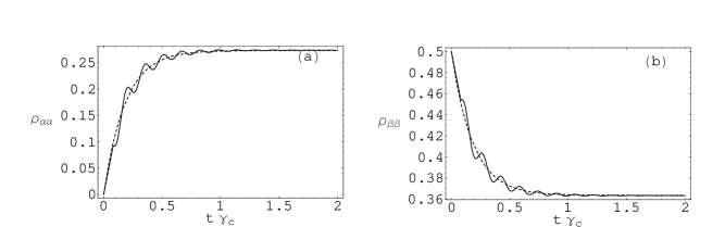
FIG. 3.: Normalized time evolution numerical simulation, of dressed state population $\rho_{\alpha\alpha}$ and $\rho_{\beta\beta}$ obtained by solving Eq.s (28) - (38) (solid line), and the approximate solution based on Eq.s (45) -(49)(dashed line) .The chosen parameters are: $\Omega=20\gamma_{c}$, $\gamma_{b}=2\gamma_{c}$, $G=0.1\gamma_{c}$, $\Lambda=3\gamma_{c}$

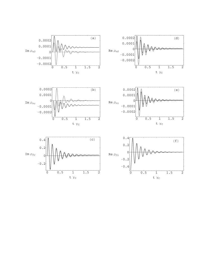
FIG. 4.: Normalized time evolution numerical simulation, of dressed state coherences obtained by solving Eq.’s (28) - (38) (solid line), and the approximate solution based on Eqs. (61) -(65) (dashed line). The chosen parameters are the same as in Fig 3

. Note the absorption despite population inversion seen in (b).

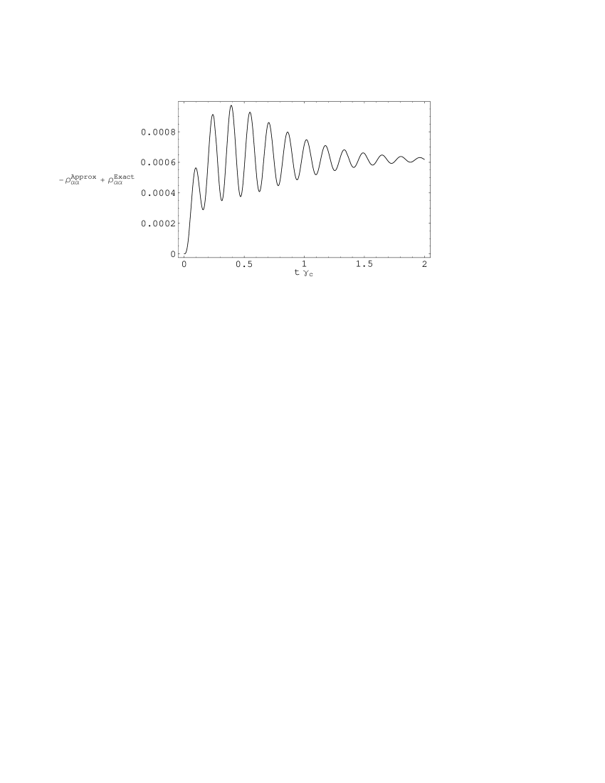
FIG. 5.: Difference between Exact population $\rho_{\alpha\alpha}$ obtained by solving Eqs. (28) - (38) and the approximate solutions based on solutions (75-77).

REFERENCES

- [1] S. E. Harris, Phys.Rev. Lett. 62, 1033 (1989).
- [2] M. O. Scully, S. Y. Zhu, and A. Gavrielides, ibid. 62, 2813 (1989).
- [3] G. S. Agrawal, Phys. Rev. A, 44, R28 (1991).
- [4] L. M. Narducci et al., Opt.Comm. 81, 379 (1991).
- [5] O. Kocharovskaya, P. Mandel, and Y. V. Radeonychev, Phys. Rev. A, 45, 1997 (1992).
- [6] Y. Zhu, Phys. Rev. A, 45, R6149 (1992).
- [7] G. Grynberg and C. Cohen - Tannoudji, Opt. Comm. 96, 150 (1993).
- [8] G. A. Wilson, K. K. Meduri, P.B. Sellin, and T. W. Mossberg, Phys. Rev. A, 50, 3394 (1994).
- [9] Gautam Vemuri, K. V. Vasavada, and G. S. Agarwal, Pys. Rev. A, 52, 3288 (1995).
- [10] Yang Zhao, Danhong Huang, and Cunkai Wu, J. Opt. Soc. Am. B 13, 1614 (1996).
- [11] N. A. Ansari and A. H. Toor, Journal of modern optics 1996, Vol. 43, No. 12, 2425 - 2435
- [12] Y. Zhu, phys. Rev. A, 53, 2742 (1996).
- [13] G. Grynberg, M. Pinard, and P. Mandel, Phys. Rev. A, 54, 776 (1996).
- [14] Gautam Vemuri and G. S. Agrawal, Phys. Rev. A, 53, 1060 (1996).
- [15] Shi - Yao Zhu, De - Zhong Wang, and Jin - Yue Gau, phys. Rev. A, 55, 1339 (1997).
- [16] Jacob B. Khurgn, and Emmanuel Rosencher, J. Opt.Soc. Am. B 14, 1249 (1997).
- [17] J. L. Cohen and P. R. Berman, Phys. Rev. A, 55, 3900 (1997).
- [18] A. S. Zibrov et al., Phys. Rev. Lett. 75, 1499 (1995).
- [19] Y. Zhu, and J. Lin, phys. Rev. A, 53, 1767 (1996).
- [20] Gautam Vemuri, G. S. Agarwal, and B. D. Nageswara, Phys. Rev. A, 54, 3695 (1996).
- [21] P. B. Sellin, G. A. Wilson, K. K. Meduri, and T. W. Mössberg, phys. Rev. A, 54, 2402 (1996).
- [22] Y. Zhu, A. I. Rubiera, and Min Xiao, Phys. Rev. A, 53, 1065 (1996)
- [23] G. S. Agarwal, Phys. Rev. Lett. 67, 980 (1991)
- [24] M. O. Scully, Phys. Rep. 219, 191 (1992)
- [25] Clude Cohen-Tanudji, Jacques Dupont-Roc and Gilbert Grynberg in Atom-Photon interactions p. 428 (John Wiley 1992)
- [26] “Mathematica” A System for Doing Mathematics by Computer , Wolfram research.
- [27] S. H. Autler and C. H. Townes, Phys. Rev., 100, 703 (19550)