Solvable potentials, non-linear algebras, and associated coherent states

Abstract

Using the Darboux method and its relation with supersymmetric quantum mechanics we construct all SUSY partners of the harmonic oscillator. With the help of the SUSY transformation we introduce ladder operators for these partner Hamiltonians and shown that they close a quadratic algebra. The associated coherent states are constructed and discussed in some detail.

Introduction

Since the early days of quantum mechanics there has been enormous interest in exactly solvable quantum systems. In fact, Schrödinger himself initiated a program GJunker:Schr40 which resulted in the famous Schrödinger-Infeld-Hull factorization method GJunker:InHu51 . In the last 10-15 years this program has been revived in connection with supersymmetric (SUSY) quantum mechanics GJunker:Jun1996 . To be a little more precise, it has been found GJunker:Gen83 that the so-called property of shape-invariance of a given Schrödinger potentials, which is in fact equivalent to the factorization condition, is sufficient for the exact solvability of the eigenvalue problem of the associated Schrödinger Hamiltonian. However, SUSY quantum mechanics has also been shown to be an effective tool in finding new exactly solvable systems. Here in essence one utilizes the fact that SUSY quantum mechanics consists of a pair of essentially isospectral Hamiltonians whose eigenstates are related by SUSY transformations. This is the basic idea of a recent construction method for so-called conditionally exactly solvable potentials GJunker:JuRo98 . Here one constructs a SUSY quantum system for which, under certain conditions imposed on its parameters, one of the SUSY partner Hamiltonians reduces to that of an exactly solvable (shape-invariant) one. Other approaches, which are also based on the presence of pairs of essentially isospectral Hamiltonians, go back to an idea formulated by Darboux GJunker:Dar1882 , are based on the inverse scattering method GJunker:AbMo80 , or on the factorization method GJunker:Mil84 . Clearly, these approaches are closely connected to each other and to the SUSY approach.

In this paper we will construct with the help of the Darboux method all possible SUSY partners of the harmonic oscillator Hamiltonian on the real line and discuss their algebraic properties in some detail. In doing so we review in the next section the Darboux method and explicitly show its equivalence to the supersymmetric approach. Section 3 then briefly presents the basic idea for the construction of conditionally exactly solvable (CES) potentials. Section 4 is devoted to a detailed discussion of the harmonic oscillator case. Here we first present all possible SUSY partners of the harmonic oscillator and give explicit expressions for the corresponding eigenstates. Secondly, with the help of the standard ladder operators of the harmonic oscillator we introduce similar ladder operators for the SUSY partners and show that they close a quadratic algebra, which is also briefly discussed. Finally, we introduce so-called non-linear coherent states which are associated with this non-linear algebra. The properties of these coherent states are discussed in some detail.

The Darboux method

In this section we briefly review the Darboux method GJunker:Dar1882 and show its connection to supersymmetric quantum mechanics GJunker:Jun1996 . In doing so we start with considering a pair of standard Schrödinger Hamiltonians acting on $L^{2}({\mathbb{R}})$,

$$H_{\pm}=-\frac{\hbar^{2}}{2m}\,\frac{\partial^{2}}{\partial x^{2}}+V_{\pm}(x)\;,$$ (1)

and a linear operator

$$A=\frac{\hbar}{\sqrt{2m}}\,\frac{\partial}{\partial x}+\Phi(x)\;,\quad\Phi:{\mathbb{R}}\to{\mathbb{R}}\;,$$ (2)

obeying the intertwining relation

$$H_{+}A=AH_{-}\;.$$ (3)

It is obvious that this intertwining relation cannot be obeyed for arbitrary functions $V_{\pm}$ and $\Phi$. In fact, the relation (3) explicitly reads

$$\begin{array}[]{r}\displaystyle\left(-\frac{\hbar^{2}}{2m}\,\Phi^{\prime\prime}(x)+V_{+}(x)\Phi(x)-\frac{\hbar}{\sqrt{2m}}\,V_{-}^{\prime}(x)-\Phi(x)V_{-}(x)\right){\bf 1}=\\[11.38109pt] \displaystyle\left(\frac{\hbar^{2}}{m}\,\Phi^{\prime}(x)+\frac{\hbar}{\sqrt{2m}}\,V_{-}(x)-\frac{\hbar}{\sqrt{2m}}\,V_{+}(x)\right)\frac{\partial}{\partial x}\;.\end{array}$$ (4)

As the unit operator ${\bf 1}$ and the momentum operator (i.e. $\partial/\partial x$) are linearly independent, their coefficients have to vanish. In other words, we are left with two conditions between the three functions $V_{\pm}$ and $\Phi$:

$$V_{-}(x)=V_{+}(x)-\frac{2\hbar}{\sqrt{2m}}\,\Phi^{\prime}(x)\;,$$ (5)

$$-\frac{\hbar^{2}}{2m}\,\Phi^{\prime\prime}(x)+V_{+}(x)\Phi(x)-\frac{\hbar}{\sqrt{2m}}\,V_{-}^{\prime}(x)-\Phi(x)V_{-}(x)=0\;.$$ (6)

Inserting the first one into the second one and integrating once we find

$$\frac{\hbar}{\sqrt{2m}}\,\Phi^{\prime}(x)-V_{+}(x)+\Phi^{2}(x)=-\varepsilon\;,$$ (7)

where $\varepsilon$ is an arbitrary real integration constant sometimes called factorization energy GJunker:Jun1996 . With this relation and with (5) we can express the two potentials under consideration in terms of the function $\Phi$:

$$V_{\pm}(x)=\Phi^{2}(x)\pm\frac{\hbar}{\sqrt{2m}}\,\Phi^{\prime}(x)+\varepsilon\;.$$ (8)

At this point one realizes that these are so-called SUSY partner potentials GJunker:Jun1996 . In fact, using relations (8) we note that

$$H_{+}=AA^{\dagger}+\varepsilon\;,\qquad H_{-}=A^{\dagger}A+\varepsilon\;.$$ (9)

These supersymmetric partner Hamiltonians are due to the intertwining relation (3) essentially isospectral, that is,

$$\mbox{spec\,}H_{+}\backslash\{\varepsilon\}=\mbox{spec\,}H_{-}\backslash\{\varepsilon\}\;.$$ (10)

Their eigenstates are related via SUSY transformations. To make this more explicit, let us denote by $|\phi^{\pm}_{n}\rangle$ the eigenstates of $H_{\pm}$ for eigenvalues $E_{n}>\varepsilon$,

$$H_{\pm}|\phi^{\pm}_{n}\rangle=E_{n}|\phi^{\pm}_{n}\rangle\;.$$ (11)

Then these states are related by SUSY transformations GJunker:Jun1996

$$|\phi^{+}_{n}\rangle=\frac{1}{\sqrt{E_{n}-\varepsilon}}\,A|\phi^{-}_{n}\rangle\;,\quad|\phi^{-}_{n}\rangle=\frac{1}{\sqrt{E_{n}-\varepsilon}}\,A^{\dagger}|\phi^{+}_{n}\rangle\;.$$ (12)

In addition to the states in (11) one of the two Hamiltonians $H_{\pm}$ may have an additional eigenstate $|\phi^{\pm}_{\varepsilon}\rangle$ with eigenvalue $\varepsilon$ obeying the first-order differential equation $A|\phi^{-}_{\varepsilon}\rangle=0$ and $A^{\dagger}|\phi^{+}_{\varepsilon}\rangle=0$, respectively. In terms of the function $\Phi$ they explicitly read

$$\phi^{\pm}_{\varepsilon}(x)=N_{\pm}\exp\left\{\pm\frac{\sqrt{2m}}{\hbar}\int dx\,\Phi(x)\right\}\;,$$ (13)

where $N_{\pm}$ stands for a normalization constant. Clearly, only one of the two solutions (13) may be square integrable. This situation corresponds to an unbroken SUSY. If none of them is square integrable then SUSY is said to be broken GJunker:Jun1996 .

The Darboux method reviewed in this section can now be used to find for a given potential, say $V_{+}$, all its possible SUSY partners $V_{-}$. Firstly, one has to solve equation (7), that is, finding all possible SUSY potentials $\Phi$. This in fact corresponds to find all possible factorizations for the corresponding Hamiltonian $H_{+}$. Finally, the corresponding SUSY partner $V_{-}$ can be obtained via (5). In this way one can construct new exactly solvable potentials. The parameters involved in the SUSY potential turn out to obey certain conditions and therefore these new potentials are more precisely called conditionally exactly solvable (CES) potentials. Let us note that the Darboux method may be generalized to intertwining operators containing higher orders of the momentum operator GJunker:AnIoSp93 .

Modelling of CES potentials

In this section we give some more details on the construction of CES potentials using the Darboux method. As just mentioned above we start with a given potential $V_{+}$ and try to find all its associated SUSY potentials. That is, we have to find the most general solution of the generalized Riccati equation (7). In doing so we will first linearize this non-linear differential equation via the substitution $\Phi(x)=(\hbar/\sqrt{2m})u^{\prime}(x)/u(x)$,

$$-\frac{\hbar^{2}}{2m}\,u^{\prime\prime}(x)+V_{+}(x)u(x)=\varepsilon u(x),$$ (14)

which is actually a Schrödinger-like equation for $V_{+}$. Note, however, that we are not restricted to normalizable solution of (14). In other words, the energy-like parameter $\varepsilon$ is up to now still arbitrary.

In terms of $u$ the linear operator $A$ reads

$$A=\frac{\hbar}{\sqrt{2m}}\left(\frac{\partial}{\partial x}+\frac{u^{\prime}(x)}{u(x)}\right)$$ (15)

and thus is only a well-defined operator on $L^{2}({\mathbb{R}})$ if $u$ does not have any zeros on the real line. As a consequence we may admit only those solutions of (14) which have no zeros. Form Sturmian theory we know that this is only possible if $\varepsilon$ is below the ground-state energy of $H_{+}$ which we will denote by $E_{0}$. Hence, we obtain a first condition on the parameter $\varepsilon$, which reads $\varepsilon<E_{0}$. This also implies that $\varepsilon$ does not belong to the spectrum of $H_{+}$. In fact, the associated eigenfunction (13) would read $\phi^{+}_{\varepsilon}(x)=N_{+}u(x)$, which is not normalizable due to condition put on $\varepsilon$.

The above condition on $\varepsilon$ is still not sufficient to guarantee a nodeless solution. Being a second-order linear differential equation (14) has two linearly independent fundamental solutions denoted by $u_{1}$ and $u_{2}$. Hence, the most general solution for $\varepsilon<E_{0}$ is given by a linear combination of the fundamental ones:

$$u(x)=\alpha\,u_{1}(x)+\beta\,u_{2}(x)\;.$$ (16)

Therefore, the condition that $u$ does not vanish also imposes conditions on the parameters $\alpha$ and $\beta$, which have to be studied case by case GJunker:JuRo98 .

Let us now assume that $H_{+}$ is an exactly solvable Hamiltonian, which means that its eigenvalues $E_{n}$ and eigenstates $|\phi^{+}_{n}\rangle$ are exactly known in closed form. For simplicity we have assumed that $H_{+}$ has a purely discrete spectrum enumerated by $n=0,1,2,\ldots$ such that $\varepsilon<E_{0}<E_{1}<\ldots$. Then via the method outlined above one can construct all its SUSY partners $H_{-}$ which are conditionally exactly solvable due to the conditions which have to be imposed on the parameters $\alpha,\beta$ and $\varepsilon$. By construction the eigenvalues of $H_{+}$ are also eigenvalues of $H_{-}$ and the corresponding eigenfunctions are obtained via the SUSY transformation (12). In the case of unbroken SUSY $H_{-}$ has one additional eigenvalue $\varepsilon$ which belongs to its ground state given by $\phi^{-}_{\varepsilon}(x)=N_{-}/u(x)$. Finally, we note that in terms of $u$ the partner potentials read

$$V_{-}(x)=\frac{\hbar^{2}}{m}\left(\frac{u^{\prime}(x)}{u(x)}\right)^{2}-V_{+}(x)+2\varepsilon$$ (17)

and form a two-parameter family label by $\varepsilon$ and $\beta/\alpha$. Note that only the quotient $\beta/\alpha$ or its inverse is relevant for (17). For various examples of CES potentials found by this method see GJunker:JuRo98 . Here we limit our discussion to those related to the harmonic oscillator.

The harmonic oscillator

In this section we will now construct all possible SUSY partner potentials for the harmonic oscillator $V_{+}(x)=(m/2)\omega^{2}x^{2}$, $\omega>0$, via the Darboux method. The corresponding Schrödinger-like equation (14) reads in this case

$$-\frac{1}{2}\,u^{\prime\prime}(x)+\frac{1}{2}\,x^{2}u(x)=\varepsilon u(x)$$ (18)

and has as general solution a linear combination of confluent hypergeometric functions

$$\textstyle u(x)=e^{-x^{2}/2}\left[\alpha\;_{1}F_{1}(\frac{1-2\varepsilon}{4},\frac{1}{2},x^{2})+\beta\;x\;_{1}F_{1}(\frac{3-2\varepsilon}{4},\frac{3}{2},x^{2})\right]\;.$$ (19)

The condition that $u$ does not have a real zero implies that $\alpha$ must not vanish and thus can be set equal to unity without loss of generality. Furthermore, $\beta$ has to obey the inequality GJunker:JuRo98 ; GJunker:CaJuTr98

$$|\beta|<\beta_{c}(\varepsilon):=2\,\frac{\Gamma(\frac{3}{4}-\frac{\varepsilon}{2})}{\Gamma(\frac{1}{4}-\frac{\varepsilon}{2})}\;.$$ (20)

The corresponding partner potentials of the harmonic oscillator then read according to (17)

$$V_{-}(x)=\left(\frac{u^{\prime}(x)}{u(x)}\right)^{2}-\frac{1}{2}\,x^{2}+2\varepsilon\;.$$ (21)

We note that for the above $u$ SUSY remains unbroken and therefore, the spectral properties of $H_{-}$ are given by

$$\begin{array}[]{l}{\mathrm{s}pec}\,H_{-}=\{\varepsilon,E_{0},E_{1},\ldots\}\quad\mbox{with}\quad E_{n}=n+\frac{1}{2}\;,\quad n=0,1,2,\ldots\;,\\[5.69054pt] \displaystyle\phi^{-}_{\varepsilon}(x)=\frac{N_{-}\,e^{x^{2}/2}}{{}_{1}F_{1}(\frac{1-2\varepsilon}{4},\frac{1}{2},x^{2})+\beta\;x\;_{1}F_{1}(\frac{3-2\varepsilon}{4},\frac{3}{2},x^{2})}\;,\\[11.38109pt] \displaystyle\phi^{-}_{n}(x)=\frac{\exp\{-x^{2}/2\}}{[\sqrt{\pi}\,2^{n+1}n!(n+1/2-\varepsilon)]^{1/2}}\left[H_{n+1}(x)+\left(\frac{u^{\prime}(x)}{u(x)}-x\right)H_{n}(x)\right]\;,\end{array}$$ (22)

where $H_{n}$ denotes the Hermite polynomial of degree $n$. Figures of the potential family (21) for various values of $\varepsilon$ and $\beta$ can be found in GJunker:JuRo98 . Here let us stress that one can even allow for complex valued $\beta\in{\mathbb{C}}\backslash[-\beta_{c}(\varepsilon),\beta_{c}(\varepsilon)]$ which in turn will give rise to complex potentials generating the same real spectrum GJunker:CaJuTr98 . We also note that the present CES potential (21) contains as special cases those previously obtain by Abraham and Moses GJunker:AbMo80 and by Mielnik GJunker:Mil84 . See also GJunker:JuRo98 for a detailed discussion.

Algebraic Structure

We will now analyse the algebraic structure for the partner Hamiltonians of the harmonic oscillator. In fact, using the standard raising and lowering operators of the harmonic oscillator $H_{+}=AA^{\dagger}+\varepsilon=a^{\dagger}a+1/2$,

$$a=\frac{1}{\sqrt{2}}\left(\frac{\partial}{\partial x}+x\right)\;,\quad a^{\dagger}=\frac{1}{\sqrt{2}}\left(-\frac{\partial}{\partial x}+x\right)\;,$$ (23)

which close the linear algebra

$$[H_{+},a]=-a\;,\quad[H_{+},a^{\dagger}]=a^{\dagger}\;,\quad[a,a^{\dagger}]={\bf 1}\;,$$ (24)

one may introduce via the SUSY transformation (12) similar ladder operators for the SUSY partners GJunker:JuRo97

$$B=A^{\dagger}aA\;,\quad B^{\dagger}=A^{\dagger}a^{\dagger}A\;,$$ (25)

which act on the eigenstates of $H_{-}$ in the following way

$$\begin{array}[]{l}B|\phi^{-}_{n+1}\rangle=\sqrt{(n+\frac{1}{2}-\varepsilon)(n+1)(n+\frac{3}{2}-\varepsilon)}|\phi^{-}_{n}\rangle\;,\\[5.69054pt] B^{\dagger}|\phi^{-}_{n}\rangle=\sqrt{(n+\frac{3}{2}-\varepsilon)(n+1)(n+\frac{1}{2}-\varepsilon)}|\phi^{-}_{n+1}\rangle\;,\\[5.69054pt] B|\phi^{-}_{0}\rangle=0\;,\quad B|\phi^{-}_{\varepsilon}\rangle=0\;,\quad B^{\dagger}|\phi^{-}_{\varepsilon}\rangle=0\;.\end{array}$$ (26)

The last two relations explicate that the ground state $|\phi^{-}_{\varepsilon}\rangle$ of $H_{-}$ is isolated in the sense that it cannot be reached via $B$ from any of the excited states and, vice versa, the excited states cannot be constructed with $B^{\dagger}$ from $|\phi^{-}_{\varepsilon}\rangle$. These ladder operators close together with the Hamiltonian $H_{-}$ the quadratic, hence non-linear, algebra

$$[H_{-},B]=-B\;,\quad[H_{-},B^{\dagger}]=B^{\dagger}\;,\quad[B,B^{\dagger}]=3H_{-}^{2}-4\varepsilon H_{-}+\varepsilon^{2}\;.$$ (27)

This quadratic algebra belongs to the class of so-called $W_{2}$ algebras and may be viewed as a polynomial deformation of the $su(1,1)$ Lie algebra. Such deformations have been discussed by Roc̆ek GJunker:Ro91 and, within a more general context, by Karassiov GJunker:Ka94 and Katriel and Quesne GJunker:KaQu96 . The quadratic Casimir operator associated with the algebra (27) reads

$$C=BB^{{\dagger}}-\Psi(H_{-})\;,\quad\Psi(H_{-})-\Psi(H_{-}-1)=3H^{2}_{-}-4\varepsilon H_{-}+\varepsilon^{2}\;.$$ (28)

In the Fock space representation (26) we have the following explicit expression

$$\Psi(H_{-})=(H_{-}-\varepsilon)(H_{-}+{\textstyle\frac{1}{2}})(H_{-}+1-\varepsilon)$$ (29)

and the relations $BB^{\dagger}=\Psi(H_{-})$ and $B^{\dagger}B=\Psi(H_{-}-1)$. Hence the Casimir (28) vanishes within this representation as expected GJunker:Ka94 ; GJunker:KaQu96 .

Non-linear coherent states

Let us now construct the non-linear coherent states GJunker:JuRo98a associated with the quadratic algebra (27). There are several ways to define such states GJunker:ZhFeGi90 . Here we will define them as eigenstates of the “non-linear” annihilation operator $B$, leading essentially to so-called Barut-Girardello coherent states GJunker:BaGi71 . We also note that the construction procedure presented below is very similar to that of coherent states associated with quantum groups GJunker:Spi95 .

Let us note that the ground state $|\phi^{-}_{\varepsilon}\rangle$ of $H_{-}$ is isolated and therefore we may construct the coherent states over the excited states $\{|\phi^{-}_{n}\rangle\}_{n\in{\mathbb{N}}_{0}}$ only. For this reason we make the ansatz

$$|\mu\rangle=\sum_{n=0}^{\infty}c_{n}\,\mu^{n}\,|\phi^{-}_{n}\rangle\;,$$ (30)

where $\mu$ is an arbitrary complex number and the real coefficients $c_{n}$ are to be determined from the defining relation

$$B|\mu\rangle=\mu\,|\mu\rangle=\sum_{n=0}^{\infty}c_{n}\,\mu^{n}\,B|\phi^{-}_{n}\rangle\;.$$ (31)

Using relations (26) we obtain the following recurrence relation for the $c_{n}$’s,

$$c_{n+1}=c_{n}\left[\textstyle(n+\frac{1}{2}-\varepsilon)(n+1)(n+\frac{3}{2}-\varepsilon)\right]^{-1/2}\;.$$ (32)

That is, the coefficients $c_{n}$ for $n\geq 1$ can be expressed in terms of $c_{0}$,

$$c_{n}=c_{0}\left[\textstyle n!(\frac{1}{2}-\varepsilon)_{n}(\frac{3}{2}-\varepsilon)_{n}\right]^{-1/2}$$ (33)

where $(z)_{n}=\Gamma(z+n)/\Gamma(z)$ denotes Pochhammer’s symbol. The remaining coefficient $c_{0}=c_{0}(\mu)$ is determined via the normalization of the coherent states

$$\langle\mu|\mu\rangle=c_{0}^{2}(\mu)\,\sum_{n=0}^{\infty}\frac{|\mu|^{2n}}{n!}\frac{1}{(\frac{1}{2}-\varepsilon)_{n}(\frac{3}{2}-\varepsilon)_{n}}=1\;.$$ (34)

Thus, we can express $c_{0}$ in terms of a generalized hypergeometric function GJunker:Erd53

$$c_{0}^{-2}(\mu)=\ _{0}F_{2}\left({\textstyle\frac{1}{2}}-\varepsilon,{\textstyle\frac{3}{2}}-\varepsilon;|\mu|^{2}\right)\;.$$ (35)

Let us now discuss some properties of these non-linear coherent states. First we note that these states are not orthogonal for $\mu\neq\nu$ as expected:

$$\langle\mu|\nu\rangle=c_{0}(\mu)\,c_{0}(\nu)\ _{0}F_{2}\left({\textstyle\frac{1}{2}}-\varepsilon,{\textstyle\frac{3}{2}}-\varepsilon;\mu^{*}\nu\right)\;.$$ (36)

Secondly, let us investigate whether these states form an overcomplete set. In other words, we consider the question: Can these states generate a resolution of the unit operator? For this we have to recall that the non-linear coherent states have been constructed over the excited states of $H_{-}$. Therefore, we start with postulating a positive measure $\rho$ on the complex $\mu$-plane obeying the following resolution of unity:

$$\int_{\mathbb{C}}d\rho(\mu^{*},\mu)\,|\mu\rangle\langle\mu|={\bf 1}-|\phi^{-}_{\varepsilon}\rangle\langle\phi^{-}_{\varepsilon}|\;.$$ (37)

Within the polar decomposition $\mu=\sqrt{x}\,e^{i\varphi}$ we make the ansatz

$$d\rho(\mu^{*},\mu)=\frac{d\varphi\,dx\,\sigma(x)}{2\pi c_{0}^{2}(\sqrt{x})}\ ,$$ (38)

with a yet unknown positive density $\sigma$ on the positive half-line. Inserting this ansatz into (37) we obtain the following conditions on $\sigma$

$$\int_{0}^{\infty}dx\,\sigma(x)\,x^{n}=\Gamma(n+1)\,\frac{\Gamma(\frac{1}{2}-\varepsilon+n)\Gamma(\frac{3}{2}-\varepsilon+n)}{\Gamma(\frac{1}{2}-\varepsilon)\Gamma(\frac{3}{2}-\varepsilon)}\;,\quad n=0,1,2,\ldots\;.$$ (39)

Hence, $\sigma$ is a probability density on the positive half-line defined by its moments given on the right-hand side of (39). Let us note that the integral in (39) may be viewed as a Mellin transformation GJunker:Erd54 of $\sigma$ and in turn the latter is given by the inverse Mellin transformation of the moments. This inverse Mellin transformation turns out to lead to the integral representation of Meijer’s G-function GJunker:Erd53 . In other words, we have the explicit form:

$$\sigma(x)=\frac{1}{\Gamma(\frac{1}{2}-\varepsilon)\Gamma(\frac{3}{2}-\varepsilon)}\,G^{30}_{03}\left(x|0,-{\textstyle\frac{1}{2}}-\varepsilon,{\textstyle\frac{1}{2}}-\varepsilon\right)\;.$$ (40)

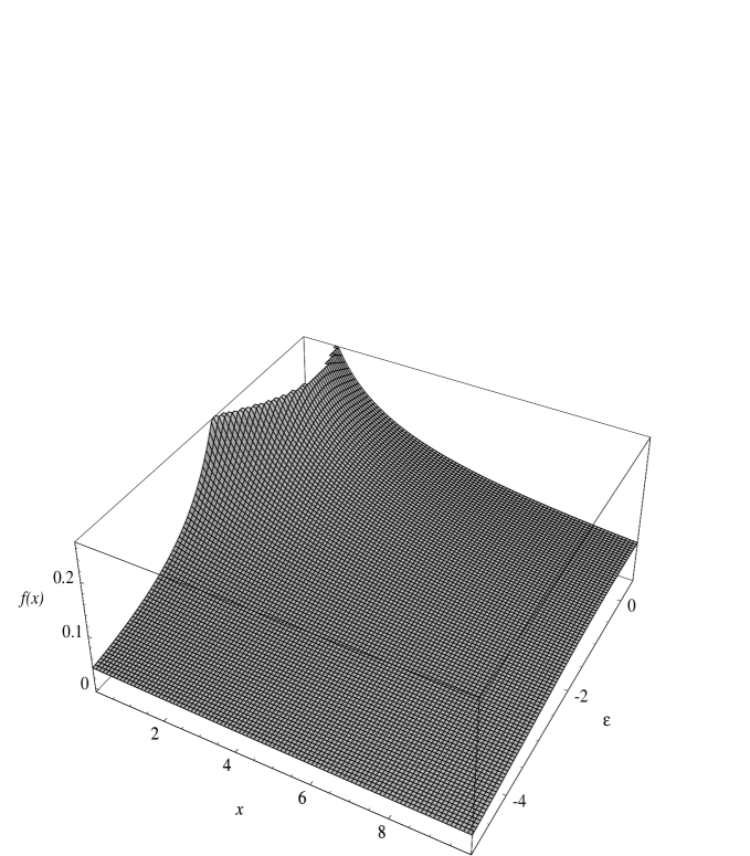
Figure 1: The radial density $f(x)=\sigma(x)/c_{0}^{2}(\sqrt{x})$ giving rise to the resolution of unity (37) with (38) as a function of $x=|\mu|^{2}$ and for various parameters $\varepsilon<\frac{1}{2}$.

In Figure 1 a plot of the radial density $f(|\mu|^{2})=2\pi\,d\rho(\mu^{*},\mu)/(d\varphi d|\mu|^{2})$ is given showing that it leads to a well-behaved positive measure on the complex $\mu$-plane.

Finally, let us point out that similar non-linear coherent states associated with the CES potentials of the radial harmonic oscillator have been constructed in GJunker:JuRo98a . In that case broken as well as unbroken SUSY can be considered and the corresponding symmetry algebra is a cubic one. In analogy to the discussion in GJunker:JuRo98a one can show that the coherent states discussed here are also minimum uncertainty states.

References

- (1) Schrödinger E., Proc. Roy. Irish Acad. 46A, 9–14 (1940); 46A, 183–206 (1941); 47A, 53–54 (1941).
- (2) Infeld L. and Hull T.E., Rev. Mod. Phys. 23, 21–68 (1951).
- (3) Junker G., Supersymmetric Methods in Quantum and Statistical Physics, Berlin: Springer-Verlag, 1996.
- (4) Gendenshteîn L.É., JETP Lett. 38, 356–358 (1983).
- (5) Junker G. and Roy P., Conditionally exactly solvable potentials: A supersymmetric construction method, preprint quant-ph/9803024.
- (6) Darboux G., Comptes Rendus Acad. Sci. (Paris) 94, 1456–1459 (1882).
-
(7)
Abraham P.B. and Moses H.E., Phys. Rev. A
22, 1333–1686 (1980).
Luban M. and Pursey D.L., Phys. Rev. D 33, 431–436 (1986).
Pursey D.L., Phys. Rev. D 33, 1048–1055 (1986). - (8) Mielnik B., J. Math. Phys. 25, 3387–3389 (1984).
-
(9)
Andrianov A.A., Ioffe M.V. and Spiridonov V.P.,
Phys. Lett. A 174, 273–179 (1993).
Andrianov A.A., Ioffe M.V., Cannata F. and Dedonder J.-P., Int. J. Mod. Phys. A 10, 2683–2702 (1995).
Samsonov B.F., J. Math. Phys. A 28, 6989–6998 (1995). - (10) Cannata F., Junker G. and Trost J., Schrödinger operators with complex potentials but real spectrum, preprint quant-ph/9805085.
-
(11)
Junker G. and Roy P., Phys. Lett. A 232,
155–161 (1997).
Junker G. and Roy P., Supersymmetric construction of exactly solvable potentials and non-linear algebras, preprint quant-ph/9709021. - (12) Roc̆ek M., Phys. Lett. B 255, 554–557 (1991).
- (13) Karassiov V.P., J. Phys. A 27, 153–165 (1994).
- (14) Katriel J. and Quesne C., J. Math. Phys. 37, 1650–1661 (1996).
- (15) Junker G. and Roy P., Non-linear coherent states associated with conditionally exactly solvable problems, preprint (1998).
- (16) Zhang W.-M., Feng D.H. and Gilmore R., Rev. Mod. Phys. 62, 867–927 (1990).
- (17) Barut A.O. and Girardello L., Commun. Math. Phys. 21, 41–55 (1971).
-
(18)
Spiridonov V., Phys. Rev. A 52,
1909–1935 (1995).
Odzijewicz A., Commun. Math. Phys. 192, 183–215 (1998). - (19) Erdélyi A., Magnus W., Oberhettinger F. and Tricomi F.G., Higher Transcedental Functions, Volume I, New York: McGraw-Hill, 1953.
- (20) Erdélyi A., Magnus W., Oberhettinger F. and Tricomi F.G., Tables of Integral Transforms, Volume I, New York: McGraw-Hill, 1954.