Nested quantum search and NP-complete problems

Abstract

A quantum algorithm is known that solves an unstructured search problem in a number of iterations of order $\sqrt{d}$, where $d$ is the dimension of the search space, whereas any classical algorithm necessarily scales as $O(d)$. It is shown here that an improved quantum search algorithm can be devised that exploits the structure of a tree search problem by nesting this standard search algorithm. The number of iterations required to find the solution of an average instance of a constraint satisfaction problem scales as $\sqrt{d^{\alpha}}$, with a constant $\alpha<1$ depending on the nesting depth and the problem considered. When applying a single nesting level to a problem with constraints of size 2 such as the graph coloring problem, this constant $\alpha$ is estimated to be around 0.62 for average instances of maximum difficulty. This corresponds to a square-root speedup over a classical nested search algorithm, of which our presented algorithm is the quantum counterpart.

I Introduction

Over the past decade there has been steady progress in the development of quantum algorithms. Most attention has focused on the quantum algorithms for finding the factors of a composite integer [1, 2] and for finding an item in an unsorted database [3, 4]. These successes have inspired several researchers to look for quantum algorithms that can solve other challenging problems, such as decision problems [5] or combinatorial search problems [6], more efficiently than their classical counterparts.

The class of NP-complete problems includes the most common computational problems encountered in practice [7]. In particular, it includes scheduling, planning, combinatorial optimization, theorem proving, propositional satisfiability and graph coloring. In addition to their ubiquity, NP-complete problems share a fortuitous kinship: any NP-complete problem can be mapped into any other NP-complete problem using only polynomial resources [7]. Thus, any quantum algorithm that speeds up the solution of one NP-complete problem immediately leads to equally fast quantum algorithms for all NP-complete problems (up to the polynomial cost of translation). Unfortunately, NP-complete problems appear to be even harder than the integer factorization problem. Whereas, classically, the best known algorithm for the latter problem scales only sub-exponentially [8], NP-complete problems are widely believed to be exponential [7]. Thus, the demonstration that Shor’s quantum algorithm [1, 2] can factor an integer in a time that is bounded by a polynomial in the “size” of the integer (i.e., the number of bits needed to represent that integer), while remarkable, does not lead to a polynomial-time quantum algorithm for NP-complete problems, the existence of which being considered as highly improbable [9]. Moreover, it has proven to be very difficult to adapt Shor’s algorithm to other computational applications.

By contrast, the unstructured quantum search algorithm [3, 4] can be adapted quite readily to the service of solving NP-complete problems. As a candidate solution to an NP-complete problem can be tested for correctness in polynomial time, one simply has to create a “database” consisting of all possible candidate solutions and apply the unstructured quantum search algorithm. Unfortunately, the speedup afforded by this algorithm is only $O(\sqrt{N})$ where $N$ is the number of candidate solutions to be tested. For a typical NP-complete problem in which one has to find an assignment of one of $b$ values to each of $\mu$ variables, the number of candidate solutions, $b^{\mu}$, grows exponentially with $\mu$. A classical algorithm would therefore take a time $O(b^{\mu})$ to find the solution whereas the unstructured quantum search algorithm would take $O(b^{\mu/2})$. Although this is an impressive speedup, one would still like to do better.

While there is now good evidence that for unstructured problems, the quantum search algorithm is optimal [9, 10, 11], these results have raised the question of whether faster quantum search algorithms might be found for problems that possess structure [6, 12, 13, 14]. It so happens that NP-complete problems have such structure in the sense that one can often build up complete solutions (i.e., value assignments for all the variables) by extending partial solutions (i.e., value assignments for a subset of the variables). Thus, rather than performing an unstructured quantum search amongst all the candidate solutions, in an NP-complete problem, we can perform a quantum search amongst the partial solutions in order to narrow the subsequent quantum search amongst their descendants. This is the approach presented in this paper and which allows us to find a solution to an NP-complete problem in a time that grows, on average, as $O(b^{\alpha\mu/2})$ for the hardest problems, where $\alpha<1$ is a constant depending on the problem instance considered.

Our improved quantum search algorithm works by nesting one quantum search within another. Specifically, by performing a quantum search at a carefully selected level in the tree of partial solutions, we can narrow the effective quantum search amongst the candidate solutions so that the net computational cost is minimized. The resulting algorithm is the quantum counterpart of a classical nested search algorithm which scales as $O(b^{\alpha\mu})$, giving a square root speedup overall. The nested search procedure mentioned here corresponds to a single level of (classical or quantum) nesting, but it can be extended easily to several nesting levels. Thus, our result suggests a systematic technique for translating a nested classical search algorithm into a quantum one, giving rise a square-root speedup, which can be useful to accelerate efficient classical algorithms (rather than a simple exhaustive search, of no practical use). We believe this technique is applicable in all structured quantum searches.

The outline of the paper is as follows. Section II introduces a simple classical tree search algorithm that exploits problem structure to localize the search for solutions amongst the candidates. This is not intended to be a sophisticated classical tree search algorithm, but rather is aimed at providing a baseline against which our quantum algorithm can be compared. In Section III, we outline the standard unstructured quantum search algorithm [3, 4]. We focus especially on the algorithm based on an arbitrary unitary search operator [15], as this is a key for implementing quantum nesting. Finally, Section IV describes the quantum tree search algorithm based on nesting, which is a direct quantum analog of the classical search algorithm appearing in Section II. The quantum search algorithm with several levels of nesting is also briefly discussed. We conclude by showing that the expected time to find a solution grows as $O(b^{\alpha\mu/2})$, that is, as the square root of the classical time for problem instances in the hard region. The constant $\alpha$, depending on the problem considered, is shown to decrease with an increasing nesting depth (i.e., an increasing number of nesting levels).

II Nested classical search on structured problems

A Structured search in trees

Many hard computational problems, such as propositional satisfiability, graph coloring, scheduling, planning, and combinatorial optimization, can be regarded as examples of so-called “constraint satisfaction problems”. Constraint satisfaction problems consist of a set of variables, each having a finite set of domain values, together with a set of logical relations (or “constraints”) amongst the variables that are required to hold simultaneously. A solution is defined by a complete set of variable/value assignments such that every variable has some value, no variable is assigned conflicting values, and all the constraints are satisfied.

In such constraint satisfaction problems, there is often a degree of commonality between different non-solutions. One typically finds, for example, that certain combinations of assignments of values to a subset of the variables are inconsistent (i.e., violate one or more of the constraints) and cannot, therefore, participate in any solution. These commonalities (several non-solutions sharing the same ancestor that is inconsistent) can be exploited to focus the search for a solution. Thus, a classical structured search algorithm can find a solution to a constraint satisfaction problem in fewer steps than that required by a unstructured search by avoiding regions of the search space that can be guaranteed to be devoid of solutions. Before investigating whether the problem structure can be exploited in a quantum search (see Sec. IV), we need to understand the circumstances under which knowledge of problem structure has the potential to be useful, classically. The key idea is that one can obtain complete solutions to a constraint satisfaction problem by systematically extending partial solutions, i.e. variable/value assignments that apply only to a subset of the variables in the problem. Not all partial solutions are equally desirable however. A partial solution is “good” if it is consistent with all the constraints against which it may be tested. Conversely a partial solution is “nogood” if it violates one or more such constraints. Sophisticated search algorithms work by incrementally extending good partial solutions and systematically terminating nogood partial solutions. This induces a natural tree-like structure on the search space of partial solutions.

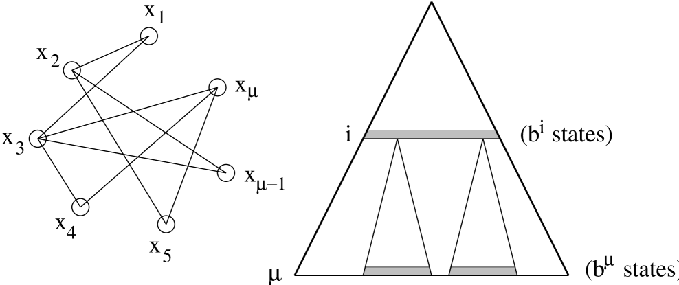
FIG. 1.: Constraint satisfaction problem in which we must find an assignment to the $\mu$ variables $x_{1},x_{2},\cdots x_{\mu}$. As an example, we picture the graph coloring problem, in which we have to assign one of $b$ possible colors to each node of a graph so that every pair of nodes that are connected directly have different colors. The corresponding search tree is characterized by a depth $\mu$ and a branching ratio $b$. By looking at partial solutions at level $i$ in the tree (the search space being of size $b^{i}$) and considering only the descendants at level $\mu$ of these partial solutions, one avoids having to search through the entire space at the bottom of the tree (of size $b^{\mu}$).

To give a concrete example of a tree search problem, we consider the graph coloring problem as pictured in Fig. 1. We have a graph that consists of $\mu$ nodes connected by $e$ edges, with $0\leq e\leq\mu(\mu-1)/2$. Each node must be assigned a color (out of $b$ possible colors), so that any two nodes connected by an edge have different colors. More generally, for a constraint satisfaction problem, we are given a set of $\mu$ variables ($x_{1},\cdots,x_{\mu}$) to which we must assign a value out of $b$ possible values. This assignment must satisfy simultaneously a set of constraints, each involving $k$ variables. The resulting number of nogood ground instances (roughly proportional to the number of constraints) is denoted by $\xi$. In the particular case of the graph coloring problem, the size of the constraints $k=2$ since each edge imposes a constraint on the colors assigned to the pair of nodes it connects. The number of nogood ground instances $\xi=eb$ because each edge contributes exactly $b$ nogoods and there are a total of $e$ edges (for each edge, $b$ pairs of identical colors are forbidden).

The search tree corresponding to this constraint satisfaction problem is also shown in Fig. 1. The $i$-th level of the search tree enumerates all possible partial solutions involving a specific subset of $i$, out of the total $\mu$, variables. The branching ratio in this tree, i.e. the number of children per node, is equal to $b$, the number of domain values of a variable. For a hard instance of the problem, the number of steps required to find a good assignment at the bottom of the tree (or decide that there is no possible assignment satisfying all the constraints) scales as $b^{\mu}$, i.e., of the order of the entire space of candidate solutions must be explored. Remarkably, many of the properties of search trees can be understood without precise knowledge of the constraints. Specifically, it has been found empirically that the difficulty of solving a particular instance of a constraint satisfaction problem can be approximately specified by four parameters: the number of variables, $\mu$, the number of values per variable, $b$, the number of variables per constraint, $k$, and the total number of assignments of the individual constraints that are nogood, $\xi$ [16, 17, 18].

Clearly, if $\xi$ is small, there are generally many solutions satisfying the few constraints, so that the problem is easy to solve. Conversely, if $\xi$ is large, the problem is in general overconstrained, and it is easy to find that it admits no solution. The problem is maximally hard in an intermediate range of values for $\xi$. In an effort to understand the observed variation in difficulty across different instances of NP-complete problems for fixed $\mu$ and $b$, it has been shown that the cost of finding a solution (or proving none exists) depends essentially on the parameter

$$\beta=\xi/\mu\,,$$ (1)

which characterizes the average number of constraints per variable [16, 19, 20]. Specifically, the problem solving difficulty exhibits a ubiquitous easy-hard-easy pattern, with the most difficult problem instances clustered around a critical value of $\beta$ given, approximately, by

$$\beta_{c}=b^{k}\log(b)$$ (2)

assuming $b^{k}\gg 1$ for simplicity. This phenomenon, akin to a phase transition in physical systems [19, 20], persists across many different sophisticated algorithms. The average case complexity for a fixed $\beta$ is therefore believed to be a more informative measure of computational complexity than either worst case or average case complexity. It is the measure that we will use in the rest of this paper for estimating the scaling of the complexity of our improved quantum search algorithm (as well as the corresponding classical search algorithm).

B Average computational complexity of a classical algorithm

Let us describe a simple classical algorithm for a tree search problem that exploits the structure of the problem by use of nesting. As pictured in Fig. 1, the key idea is to perform a preliminary search through a space of partial solutions in order to avoid a search through the entire space at the bottom of the tree. By definition, a partial solution at level $i$ in the tree assigns values to a subset of $i$ so-called primary variables ($x_{1},\cdots,x_{i}$), which we denote as $A$. The subset of secondary variables ($x_{i+1},\cdots,x_{\mu}$), denoted as $B$, corresponds to the variables to which we assign a value only when extending the partial solutions (i.e., when considering the descendants of the partial solutions). In general, any partial solution can be tested against a part of the constraints, namely just those constraints involving the primary variables $A$. A partial solution that satisfies all these (testable) constraints can be viewed as a could-be solution in the sense that all solutions at the bottom of the tree (at level $\mu$) must be descendants of could-be’s. A classical search can be speeded up by terminating search along paths that are not descendants of a could-be, thereby avoiding to search through the entire space. The following algorithm can be used:

• Find a could-be solution at level $i$ in the tree. For this purpose, choose repeatedly a random partial solution at level $i$, until it satisfies the testable constraints.

• For each could-be solution, check exhaustively (or by use of a random search) all its descendants at the bottom of the tree (level $\mu$) for the presence of a possible solution.

This is clearly not a sophisticated algorithm. It amounts to nesting the search for a successful descendant at level $\mu$ into the search for a could-be at level $i$. Nevertheless, it does exploit the problem structure by using the knowledge gleaned from the search at level $i$ to focus the search at level $\mu$. By finding a quantum analog of this algorithm (cf. Sec. IV), we will, therefore, be able to address the impact of problem structure on quantum search.

Let us estimate the expected cost of running this algorithm. This cost consists essentially of three components: $n$, the cost of finding a consistent partial solution (a could-be) at level $i$ in the tree, $m$, the cost of the subsequent search among its descendants at level $\mu$, and $r$, the number of repetitions of this whole procedure before finding a solution. The search space for partial solutions (assignment of the primary variables $A$) is of size $d_{A}=b^{i}$. Assuming that there are $n_{A}$ could-be solutions at level $i$ (i.e., partial solutions that can lead to a solution), the probability of finding one of them by using a random search is thus $n_{A}/d_{A}$. Thus, one needs of the order of

$$n=d_{A}/n_{A}$$ (3)

iterations to find one could-be solution. The descendants of a could-be are obtained by assigning a value to the subset of secondary variables $B$, of size $d_{B}=b^{\mu-i}$ (each could-be has $d_{B}$ descendants). Thus, searching through the entire space of descendants of a could-be requires on average

$$m=d_{B}$$ (4)

iterations. If the problem admits a single solution, this whole procedure needs to be repeated $n_{A}$ times, on average, since we have $n_{A}$ could-be solutions. More generally, if the number of solutions of the problem is given by $n_{AB}$, this procedure must only be repeated

$$r=n_{A}/n_{AB}$$ (5)

times in order to find a solution with a probability of order 1. Thus, the total number of iterations required to find a solution of an average instance is approximately equal to

$$T_{c}\simeq r(n+m)={d_{A}+n_{A}d_{B}\over n_{AB}}$$ (6)

This corresponds to an improvement over a naive unstructured search algorithm. Indeed, the cost of a naive algorithm that does not exploit structure is simply $d_{AB}/n_{AB}$, where $d_{AB}=d_{A}d_{B}=b^{\mu}$ is the dimension of the total search space.

The first term in the numerator of Eq. (6) corresponds to the search for could-be solutions in a space of partial solutions of size $d_{A}$ (shaded area at level $i$ in Fig. 1), while the second term corresponds to the search for actual solutions among all the descendants of the $n_{A}$ could-be solutions, each of them having $d_{B}$ descendants (shaded area at level $\mu$ in Fig. 1). The denominator in Eq. (6) accounts for a problem admitting more than one solution. We will see in Sec. IV that the quantum counterpart of Eq. (6) involves taking the square root of $n$, $m$, and $r$, which essentially results in quantum-mechanical square-root speedup over this classical algorithm.

To make the estimate of this classical average-case complexity more quantitative, let $p(i)$ be the probability that a partial solution at level $i$ is “good” (i.e., that it satisfies all the testable constraints). In Appendix A, we provide an asymptotic estimate of $p(i)$ for an average instance of a large problem ($\mu\to\infty$) with a fixed value of the parameter $\beta$. Recall that, if we want to preserve the difficulty while considering the limit of large problems, $\beta$ must be kept constant. This is necessary for the complexity measure that we consider in this paper, as mentioned before. Thus, by making use of this asymptotic estimate of $p(i)$, we can approximate the expected number of could-be solutions at the $i$th level, $n_{A}=p(i)b^{i}$, and the expected number of solution at the bottom of the tree, $n_{AB}=p(\mu)b^{\mu}$. Therefore, the average search time of the classical algorithm to find the first solution is approximately equal to

$$T_{c}(i)={b^{i}+p(i)b^{\mu}\over p(\mu)b^{\mu}}$$ (7)

This is essentially the cost for finding one solution (which basically requires checking all the partial solutions for a could-be, and subsequently checking the descendants of all these could-be solutions) divided by the expected number of solutions.

Equation (7) yields an approximate cost measure for our classical nested search algorithm as a function of the level of the “cut”, $i$. An important question now is where to cut the search tree? If one cuts the tree too high (searching for could-be solutions at small $i$), one is unlikely to learn anything useful as most partial solutions will probably be “goods”, allowing for little discrimination between solutions and non-solutions. In other words, the second term in the numerator of Eq. (7) dominates since $p(i)$ is close to 1, i.e., there are many could-be solutions at level $i$. Searching for could-be solutions is thus fast (the space of primary variables is of size $b^{i}$ only), but those partial solutions are of little use for singling out the actual solutions. The cost of the search among the descendants of those partial solutions is then high. Conversely, if one cuts the tree too deep (searching for could-be solutions at large $i$), although this would enhance discrimination between solutions and non-solutions, the search space for the primary variables would be almost as large as the entire space. Then, the first term dominates the scaling as the search for could-be solutions becomes time-consuming. It is therefore apparent that, for a typical problem instance, there ought to be an optimal level at which to cut.

We can estimate the optimal level by finding the value of $i$ that minimizes the classical computation time $T_{c}(i)$ for a given value of $\mu$, $b$, $\xi$, and $k$, using the functional form for $p(i)$. This is done in Appendix B, where we estimate the asymptotic behavior of the location of the optimal cut level as a function of $\beta$, as larger problems are considered ($\mu\to\infty$). We then calculate the corresponding asymptotic scaling of $T_{c}$ for large problems. The result is that the computation cost of running the classical nested search algorithm scales as

$$T_{c}\simeq b^{\alpha\mu}$$ (8)

for a search space of dimension $d=b^{\mu}$, where $\alpha<1$ is a constant depending on the problem considered. (More generally, this constant also depends on the number of nesting levels, but we have considered a single level of nesting in this Section.) As we will see, the structured quantum search algorithm that we present in Sect. IV has a computational cost of order of $\sqrt{b^{\alpha\mu}}$, in agreement with the idea that a square root speedup is the best that can be achieved by quantum mechanics. The focus of this paper, however, is to show explicitly how a quantum algorithm can be implemented that reaches this maximum speedup over the classical algorithm discussed above. Interestingly enough, the quantum complexity of our nested algorithm scales then as a power of the dimension of the search space $d=b^{\mu}$ that is less than 1/2. Structured quantum search therefore offers a significant speedup over both structured classical search and unstructured quantum search.

III Unstructured quantum search

Let us first review the standard unstructured quantum search algorithm [3, 4]. Consider a Hilbert space of dimension $d$ in which each basis $|x\rangle$ state ($x=1,\cdots d$) corresponds to a candidate solution of a search problem. Any search problem can be recast as the problem of finding the value(s) of $x$ at which an “oracle” function $f(x)$ is equal to one (this function being zero elsewhere). We start the quantum search process from an arbitrary basis state $|s\rangle$, and the goal is to reach a solution (or target) basis state $|t\rangle$, with $f(t)=1$, in a shortest computation time. More precisely, if there is a single solution (or target state), the goal is to reach a state that has an amplitude of order 1 in $|t\rangle$, so that a measurement of this state gives the solution with probability of order 1. (If there are $r$ solutions, the goal is to reach a superposition of the states $|t\rangle$, each with an amplitude of order $r^{-1/2}$.)

The quantum search algorithm we discuss below is in fact an immediate extension of the original one [3, 4], where an arbitrary unitary transformation is used instead of the Walsh-Hadamard transformation [15]. Assume that we have at our disposal a quantum circuit that performs a particular unitary operation $U$. If this operation connects the starting state $|s\rangle$ to the target state $|t\rangle$, i.e., $\langle t|U|s\rangle\neq 0$, then this operation can be used classically to find the target. Indeed, if we measure the system after applying $U$, the probability of obtaining the solution $|t\rangle$ is obviously $|\langle t|U|s\rangle|^{2}$. Thus, on average, we need to repeat this experiment $|\langle t|U|s\rangle|^{-2}$ times to find the solution with probability of order 1. We will show now that, using a quantum algorithm, it is possible to reach the target state $|t\rangle$ in a number of steps of order $|\langle t|U|s\rangle|^{-1}$ only, which represents a huge speedup provided that $|\langle t|U|s\rangle|\ll 1$ (this corresponds to the situation of interest where the search space is very large).

The idea behind a quantum search algorithm is to postpone the measurement, and keep a superposition of quantum states throughout the algorithm. Only at the end, a measurement is performed. Let us define the unitary operation

$$Q=-UI_{s}U^{\dagger}I_{t}=-U\,e^{\displaystyle i\pi P_{s}}\,U^{\dagger}\,e^{\displaystyle i\pi P_{t}}$$ (9)

where $P_{s}=|s\rangle\langle s|$ and $P_{t}=|t\rangle\langle t|$ are projection operators on $|s\rangle$ and $|t\rangle$, respectively. The two unitary operators $I_{s}=\openone-2P_{s}$ and $I_{t}=\openone-2P_{t}$ perform a controlled-phase operation: applying $I_{s}$ (or $I_{t}$) on a state $|x\rangle$ flips its phase if $x=s$ (or $x=t$), and leaves it unchanged otherwise. Note that the target state $|t\rangle$ is of course not available (it is what we are searching for). Instead, we have at our disposal the quantum circuit (or “oracle”) that computes the function $f(x)$, and we can use it to implement the circuit for $I_{t}$. Thus, we have $I_{t}|x\rangle=(-1)^{f(x)}|x\rangle$ for all state $|x\rangle$. The circuit for $I_{s}$ does not require the function $f(x)$ and is trivial. The principle at the heart of quantum search is to apply the operation $Q$ repeatedly in order to amplify the target component $|t\rangle$, starting from $U|s\rangle$. This quantum amplitude amplification [21] can be understood by noting that, after applying $U$ to the starting state $|s\rangle$, the repeated applications of $Q$ essentially rotate this state into the target state $|t\rangle$ at an angular velocity that is linear in the number of iterations. More specifically, using $Q=-\openone+2|t\rangle\langle t|+2U|s\rangle\langle s|U^{\dagger}-4U|s\rangle\langle s|U^{\dagger}|t\rangle\langle t|$, we can see that $Q$ preserves the two-dimensional subspace spanned by $U|s\rangle$ and $|t\rangle$, namely

$$Q\left(\begin{array}[]{c}U|s\rangle\\ |t\rangle\end{array}\right)=\left(\begin{array}[]{cc}1-4\,|\langle t|U|s\rangle|^{2}&2\langle t|U|s\rangle\\ -2\langle t|U|s\rangle^{*}&1\end{array}\right)\;\left(\begin{array}[]{c}U|s\rangle\\ |t\rangle\end{array}\right)$$ (10)

Therefore, in the case where $|\langle t|U|s\rangle|\ll 1$, the states $U|s\rangle$ and $|t\rangle$ are almost orthogonal, and $Q$ tends to a rotation matrix of angle $2|\langle t|U|s\rangle|\ll 1$. Indeed, keeping only the first-order terms in $u\equiv\langle t|U|s\rangle$, we obtain

$$Q\left(\begin{array}[]{c}U|s\rangle\\ |t\rangle\end{array}\right) \simeq \left(\begin{array}[]{cc}1&2u\\ -2u^{*}&1\end{array}\right)\;\left(\begin{array}[]{c}U|s\rangle\\ |t\rangle\end{array}\right)$$ (17)

$$\simeq \exp\left(\begin{array}[]{cc}0&2u\\ -2u^{*}&0\end{array}\right)\;\left(\begin{array}[]{c}U|s\rangle\\ |t\rangle\end{array}\right)$$ (22)

We can then easily approximate the operation of $Q^{n}$ in the subspace spanned by $U|s\rangle$ and $|t\rangle$:

$$Q^{n}\left(\begin{array}[]{c}U|s\rangle\\ |t\rangle\end{array}\right) \simeq \exp\left(\begin{array}[]{cc}0&2nu\\ -2nu^{*}&0\end{array}\right)\;\left(\begin{array}[]{c}U|s\rangle\\ |t\rangle\end{array}\right)$$ (29)

$$\simeq \left(\begin{array}[]{cc}\cos(2n|u|)&{\displaystyle u\over\displaystyle|u|}\sin(2n|u|)\\ -{\displaystyle u^{*}\over\displaystyle|u|}\sin(2n|u|)&\cos(2n|u|)\end{array}\right)\;\left(\begin{array}[]{c}U|s\rangle\\ |t\rangle\end{array}\right)$$ (34)

implying that the amplitude of the target state $|t\rangle$ after $n$ iterations is

$$\langle t|Q^{n}U|s\rangle\;\simeq\;u\,\cos(2n|u|)+{\displaystyle u\over\displaystyle|u|}\sin(2n|u|)$$ (35)

These last expressions are only asymptotically valid, at the limit of small $|u|$. The exact expressions for Eqs. (34) and (35) in terms of Chebyshev polynomials can be found in Appendix C.

Consider first the case of a small rotation angle. From Eq. (35), we see that if we iterate the application of $Q$ on $U|s\rangle$, the amplitude of $|t\rangle$ grows linearly with the number of iterations $n$ provided that the total angle $2n|u|\ll 1$:

$$\langle t|Q^{n}U|s\rangle\;\simeq\;(1+2n)\;\langle t|U|s\rangle$$ (36)

Consequently, if we measure the system after $n$ iterations, the probability $p(n)$ of finding the solution grows quadratically with $n$, as $p(n)\sim n^{2}|\langle t|U|s\rangle|^{2}$. This is a great improvement compared to the linear scaling of the classical algorithm consisting in repeating $n$ times the measurement of $U|s\rangle$, namely $p(n)\sim n|\langle t|U|s\rangle|^{2}$. This is the quadratic amplification effect provided by quantum mechanics.

Now, consider the goal of reaching the target state $|t\rangle$ using this operator $Q$. From Eq. (29) we see that, starting from the state $U|s\rangle$, we need to apply $Q$ until we have rotated it by an angle of about $\pi/2$ in order to reach $|t\rangle$. At this time only, one measures the system and gets the desired solution with a probability of order 1. The number of iterations required to rotate $U|s\rangle$ into the solution $|t\rangle$ is thus

$$n\simeq{\pi\over 4}\;|\langle t|U|s\rangle|^{-1}$$ (37)

and scales as the square root of the classical time. It is worth noting that the amplitude of any state $|x\rangle$ orthogonal to the target $|t\rangle$ is given by

$$\langle x|Q^{n}U|s\rangle\simeq\cos(2n|u|)\,\langle x|U|s\rangle$$ (38)

so that $\langle x|Q^{n}U|s\rangle\simeq\langle x|U|s\rangle$ for small angles. Thus, the amplitude of non-solutions is not amplified by applying $Q$ repeatedly, so that the quantum search algorithm selectively amplifies the solutions only.

Thus, we have described here a general technique for achieving a quantum-mechanical square-root speedup of a search algorithm relying on any unitary transformation $U$ [15]. The quantum search algorithm can be simply viewed as a rotation from $U|s\rangle$ to $|t\rangle$ based on the repeated operation of $Q$, followed by a measurement. In the above discussion, the search operator $U$ can be arbitrary, provided it connects $|s\rangle$ and $|t\rangle$. In the case of an unstructured search problem, as we have no a priori knowledge about where the solution is located, the most natural choice for $U$ is the Walsh-Hadamard transformation $H$ [3, 4]:

$$H|x\rangle={1\over\sqrt{d}}\sum_{y=0}^{d-1}(-1)^{\overline{x}\cdot\overline{y}}|y\rangle$$ (39)

where $\overline{x}\cdot\overline{y}=\sum_{i=0}^{d-1}x_{i}y_{i}({\rm mod}~{}2)$, with $x_{i}$ ($y_{i}$) being the binary digits of $x$ ($y$). Indeed, $U=H$ does not bias the search towards a particular candidate solution since $H|s\rangle$ has the same (squared) amplitude in all the candidate solutions, so that the search starts from a uniform distribution of all states. Applying $U=H$ to an arbitrary state $|s\rangle$, we see that

$$\langle t|H|s\rangle=\pm 1/\sqrt{d}$$ (40)

for all possible target state $|t\rangle$. Thus, according to Eq. (37), the number of iterations in the quantum search algorithm relying on $H$ is $O(\sqrt{d})$ [3, 4], whereas a classical search algorithm obviously requires $O(d)$ steps. When there are multiple target states (the problem admits several solutions), it can be shown that the quantum computation time becomes $O(\sqrt{d/r})$, where $r$ is the number of solutions [10]. The classical counterpart is then simply $O(d/r)$.

For a structured search problem, however, it is natural to use the knowledge of the structure in order to choose a better $U$. Indeed, if we have partial knowledge about where the solutions are, we can exploit it to bias the search in such a way that $U|s\rangle$ has larger amplitudes in states which are more probable to be solutions. This is the focus of the present paper. It has been shown recently that an arbitrary (non-uniform) initial amplitude distribution can be used as well with the standard quantum search algorithm, resulting in a $O(\sqrt{d/r})$ quantum computation time [22]. This seems to indicate that the scaling remains in $O(\sqrt{d})$ even if we use our knowledge about the problem by biasing the initial distribution. In contrast, we will show in Sec. IV that the use of a nested quantum search algorithm can result in a power law in $d$ with an exponent that is smaller than 1/2. The key idea is that $U$ is not fixed a priori, but is rather obtained “dynamically” by the quantum algorithm itself, depending on the particular instance. In short, the standard search algorithm is used to construct an effective search operator $U$ (or a non-uniform initial distribution) which, itself, is nested within another quantum search algorithm. In other words, we apply quantum search “recursively”: the operator $(-HI_{s}HI_{t})^{n}H$ resulting from the nested search algorithm based on $H$ is used as a better search operator $U$ for a quantum search at an upper level of hierarchy.

IV Nested quantum search on structured problems

A The core quantum algorithm

Assume that the Hilbert space of our search problem is the tensor product of two Hilbert spaces ${\cal H}_{A}$ and ${\cal H}_{B}$. As before, $A$ denotes the set of primary variables, that is, the variables to which we assign a value in the first stage. The partial solutions correspond to definite values for these variables. Thus, ${\cal H}_{A}$ represents the search space for partial solutions (of dimension $d_{A}$). The set of secondary variables, characterizing the extensions of partial solutions, is denoted by $B$, and the corresponding Hilbert space ${\cal H}_{B}$ is of dimension $d_{B}$. Let us briefly describe the quantum algorithm with a single nesting level (the counterpart of the classical algorithm of Sect. II):

• The first stage (i) consists in constructing a superposition (with equal amplitudes) of all the could-be solutions at level $i$ by use of the standard unstructured search algorithm based on $H$.

• Then (ii), one performs a subsequent quantum search in the subspace of the descendants of all the could-be partial solutions, simultaneously. This second stage is achieved by using the standard quantum search algorithm with, as an input, the superposition of could-be solutions resulting from the first stage. The overall yield of stages (i) and (ii) is a superposition of all states where the solutions have been partially amplified with respect to non-solutions.

• The final procedure (iii) consists of nesting stages (i) and (ii)— using them as a search operator $U$—inside a higher-level quantum search algorithm until the solutions get maximally amplified, at which point a measurement is performed. This is summarized in Fig. 2.

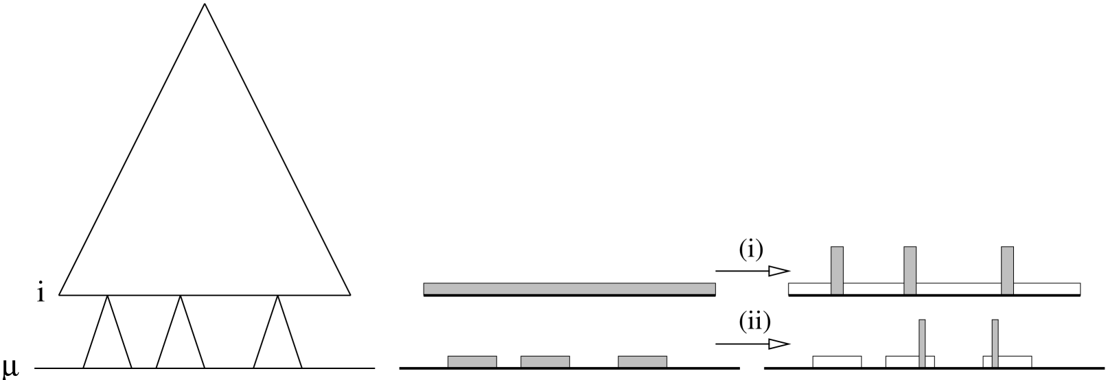
FIG. 2.: Schematic representation of stages (i) and (ii) of the quantum algorithm. These stages partially amplify the solution states, and can be nested into a standard quantum search algorithm (iii) in order to speedup the amplification of the solutions.

Let us now follow in more details the evolution of the quantum state by applying this quantum nested algorithm, and estimate the number of iterations required. The starting state of the search is denoted as $|s,s^{\prime}\rangle$, where $|s\rangle$ (lying in ${\cal H}_{A}$) and $|s^{\prime}\rangle$ (lying in ${\cal H}_{B}$) are just the initial state of two different parts of the same, single, quantum register which is large enough to hold all the potential solutions in the total search space (i.e.. all the $b^{\mu}$ leaf nodes of the search tree at level $\mu$). Register $A$ stores the starting state at an intermediate level $i$ in the tree, while register $B$ stores the continuation of that state at level $\mu$. In other words, $A$ holds partial solutions and $B$ their elaboration in the leaves of the tree.

(i) The first stage of the algorithm consist in a standard quantum search for could-be partial solutions $|c\rangle$ at level $i$, that is, states in subspace ${\cal H}_{A}$ that do not violate any (testable) constraint. We start from state $|s\rangle$ in subspace ${\cal H}_{A}$, and apply a quantum search based on the Walsh-Hadamard transformation $H$ since we do not have a priori knowledge about the location of could-be solutions. Using

$$\langle c|H|s\rangle=\pm 1/\sqrt{d_{A}}$$ (41)

we can perform an amplification of the components $|c\rangle$ based on $Q=-HI_{s}HI_{c}$ where

$$I_{s} = \exp(i\pi|s\rangle\langle s|)$$ (42)

$$I_{c} = \exp(i\pi\sum_{c\in C}|c\rangle\langle c|)$$ (43)

The states $|c\rangle$ correspond to the could-be partial solutions in ${\cal H}_{A}$ (assignment of the primary variables that could lead to a solution), and belong to the subset $C=\{c_{1},\cdots,c_{n_{A}}\}$. We assume that there are $n_{A}$ could-be partial solutions, with $1\ll n_{A}\ll d_{A}$. The quadratic amplification of these could-be solutions, starting from $|s\rangle$, is reflected by

$$\langle c|Q^{n}H|s\rangle\simeq n\;\langle c|H|s\rangle\simeq n/\sqrt{d_{A}}$$ (44)

for small rotation angle. Thus, applying $Q$ sequentially, we can construct a superposition of all the could-be solutions $|c\rangle$, each with an amplitude of order $\sim 1/\sqrt{n_{A}}$. The required number of iterations of $Q$ scales as

$$n\simeq\sqrt{d_{A}/n_{A}}$$ (45)

This amplitude amplification process can equivalently be described in the joint Hilbert space ${\cal H}_{A}\otimes{\cal H}_{B}$, starting from the product state $|s,s^{\prime}\rangle$, where $|s^{\prime}\rangle$ denotes an arbitrary starting state in ${\cal H}_{B}$, and applying $(Q\otimes\openone)$ sequentially:

$$\langle c,s^{\prime}|(Q\otimes\openone)^{n}(H\otimes\openone)|s,s^{\prime}\rangle=\langle c|Q^{n}H|s\rangle\sim n/\sqrt{d_{A}}$$ (46)

Here and below, we use the convention that the left (right) term in a tensor product refers to subspace $A$ ($B$).

(ii) The second stage of the algorithm is a standard quantum search for the secondary variables $B$ in the subspace of the “descendants” of the could-be solutions that have been singled out in stage (i). As before, we can use the search operator $H$ that connects extended could-be solutions $|c,s^{\prime}\rangle$ to the actual solutions or target states $|t,t^{\prime}\rangle$ in the joint Hilbert space:

$$\langle t,t^{\prime}|(\openone\otimes H)|c,s^{\prime}\rangle=\langle t|c\rangle\,\langle t^{\prime}|H|s^{\prime}\rangle=\pm\delta_{\displaystyle c,t}/\sqrt{d_{B}}$$ (47)

Note that, this matrix element is non-vanishing only for could-be states $|c\rangle$ that lead to an actual solution. Define the operator $R=-(\openone\otimes HI_{s^{\prime}}H)I_{t}$, with

$$I_{s^{\prime}} = \exp\big{(}i\pi|s^{\prime}\rangle\langle s^{\prime}|\big{)}$$ (48)

$$I_{t\phantom{{}^{\prime}}} = \exp\big{(}i\pi\sum_{(t,t^{\prime})\in T}|t,t^{\prime}\rangle\langle t,t^{\prime}|\big{)}$$ (49)

where $T$ is the set of solutions $|t,t^{\prime}\rangle$ at the bottom of the tree, and $\#(T)=n_{AB}$, i.e., the problem admits $n_{AB}$ solutions. We can apply the operator $R$ sequentially in order to amplify a target state $|t,t^{\prime}\rangle$, namely

$$\langle t,t^{\prime}|R^{m}(\openone\otimes H)|c,s^{\prime}\rangle\simeq\left\{\begin{array}[]{l @{\qquad} l}m\;\langle t,t^{\prime}|(\openone\otimes H)|c,s^{\prime}\rangle&{\rm if~{}}c=t\\ \langle t,t^{\prime}|(\openone\otimes H)|c,s^{\prime}\rangle&{\rm if~{}}c\neq t\end{array}\right.$$ (50)

for small rotation angle. Note that, for a could-be state $|c\rangle$ that does not lead to a solution ($c\neq t$), we have $I_{t}|c,x\rangle=|c,x\rangle$ for all $x$, so that $R^{m}(\openone\otimes H)|c,s^{\prime}\rangle=(-\openone\otimes HI_{s^{\prime}}H)^{m}(\openone\otimes H)|c,s^{\prime}\rangle=(\openone\otimes H)|c,s^{\prime}\rangle$, and the matrix element is not amplified by $m$ compared to the case $c=t$. In other words, no amplification occurs in the space of descendants of could-be partial solutions that do not lead to an actual solution. Thus, Eq. (50) results in

$$\langle t,t^{\prime}|R^{m}(\openone\otimes H)|c,s^{\prime}\rangle\simeq{m\over\sqrt{d_{B}}}\delta_{\displaystyle c,t}$$ (51)

Assuming that, among the descendants of each could-be solution $|c,s^{\prime}\rangle$, there is either zero or one solution, we need to iterate $R$ of the order of

$$m\simeq\sqrt{d_{B}}$$ (52)

times in order to maximally amplify each solution. We then obtain a superposition of the solution states $|t,t^{\prime}\rangle$, each with an amplitude $\sim 1/\sqrt{n_{A}}$. This can also be seen by combining Eqs. (46) and (51), and using the resolution of identity $\openone=\sum_{x,y}|x,y\rangle\langle x,y|$:

$$\langle t,t^{\prime}|\underbrace{R^{m}(\openone\otimes H)(Q\otimes\openone)^{n}(H\otimes\openone)}_{U}|s,s^{\prime}\rangle = \sum_{x,y}\langle t,t^{\prime}|R^{m}(\openone\otimes H)|x,y\rangle\,\langle x,y|(Q\otimes\openone)^{n}(H\otimes\openone)|s,s^{\prime}\rangle$$ (53)

$$= \langle t,t^{\prime}|R^{m}(\openone\otimes H)|t,s^{\prime}\rangle\,\langle t,s^{\prime}|(Q\otimes\openone)^{n}(H\otimes\openone)|s,s^{\prime}\rangle$$ (54)

$$\simeq (m/\sqrt{d_{B}})(n/\sqrt{d_{A}})$$ (55)

$$\simeq 1/\sqrt{n_{A}}$$ (56)

Thus, applying the operator $Q^{n}$ followed by the operator $R^{m}$ connects the starting state $|s,s^{\prime}\rangle$ to each of the solutions $|t,t^{\prime}\rangle$ of the problem with a matrix element of order $\sim 1/\sqrt{n_{A}}$.

(iii) The third stage consists in using the operator $U\equiv R^{m}(\openone\otimes H)(Q\otimes\openone)^{n}(H\otimes\openone)$ resulting from steps (i) and (ii) as a search operator for a higher-level quantum search algorithm, in order to further amplify the superposition of $n_{AB}$ target (or solution) states $|t,t^{\prime}\rangle$. The goal is thus to construct such a superposition where each solution has an amplitude of order $\sim 1/\sqrt{n_{AB}}$. As before, we can make use of the operator $S=-U(I_{s}\otimes I_{s^{\prime}})U^{\dagger}I_{t}$ where $I_{s}$, $I_{s^{\prime}}$, and $I_{t}$ are defined in Eqs. (42), (48), and (49), in order to perform amplification according to the relation

$$\langle t,t^{\prime}|S^{r}U|s,s^{\prime}\rangle\simeq r\;\langle t,t^{\prime}|U|s,s^{\prime}\rangle\simeq r/\sqrt{n_{A}}$$ (57)

for small rotation angle. The number of iterations of $S$ required to maximally amplify the solutions is thus of the order of

$$r\simeq\sqrt{n_{A}\over n_{AB}}$$ (58)

This completes the algorithm. At this point, it is sufficient to perform a measurement of the amplified superposition of solutions. This yields one solution $|t,t^{\prime}\rangle$ with a probability of order 1.

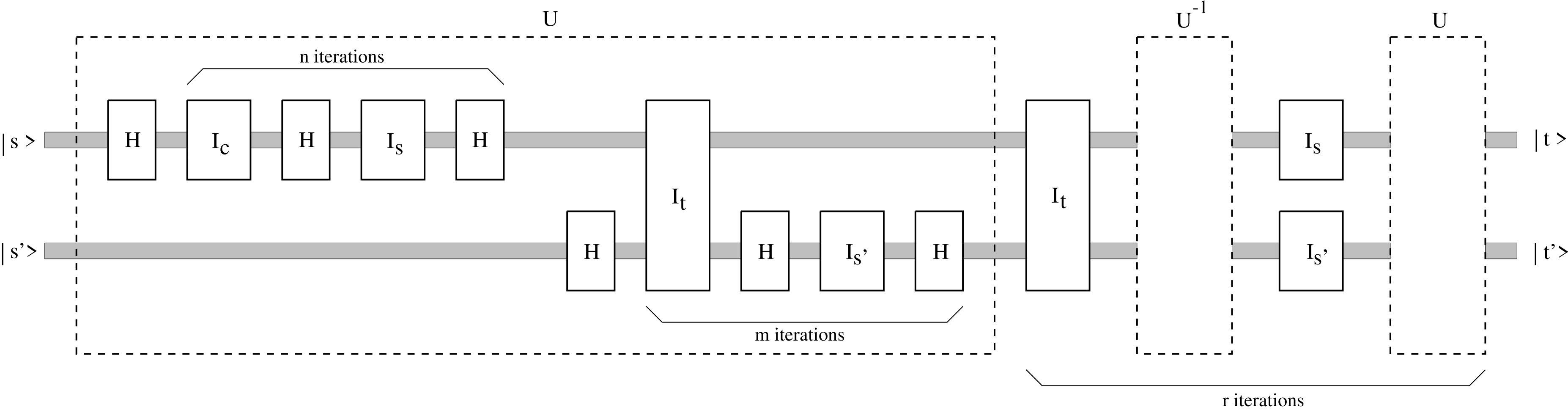
FIG. 3.: Circuit implementing the nested quantum search algorithm (with a single level of nesting). The upper set of quantum variables, initially in state $|s\rangle$, corresponds to the primary variables $A$. The lower set of quantum variables, initially in states $|s^{\prime}\rangle$, is associated with the secondary variables $B$. The quantum circuit makes use of controlled-phase gates $I_{s}=\exp(i\pi|s\rangle\langle s|)$, $I_{s^{\prime}}=\exp(i\pi|s^{\prime}\rangle\langle s^{\prime}|)$, $I_{c}=\exp(i\pi\sum_{c\in C}|c\rangle\langle c|)$, and $I_{t}=\exp(i\pi\sum_{(t,t^{\prime})\in T}|t,t^{\prime}\rangle\langle t,t^{\prime}|)$, and Walsh-Hadamard gates $H$. The entire operation of $U$ (exhibited inside the dashed box) is repeated $r$ times. Note that $U^{-1}=U^{\dagger}$ corresponds to same the circuit as $U$ but read from right to left.

In Fig. 3, the quantum network that implements this nested quantum search algorithm is illustrated. Clearly, a sequence of two quantum search circuits (a search in the $A$ space followed by a search in the $B$ space) is nested into a global search circuit in the whole Hilbert space ${\cal H}_{AB}$. This can be interpreted as a “dynamical” choice of the search operator $U$ that is used in the global quantum search. This quantum nesting is distinct from a procedure where one would try to choose an optimum $U$ before running the quantum search by making use of the structure classically (making several classical queries to the oracle) in order to speedup the resulting quantum search. Here, no measurement is involved and structure is used at the quantum level.

B Quantum average-case complexity

Let us estimate the total number of iterations, or more precisely the number of times that a controlled-phase operator ($I_{t}$, which flips the phase of a solution, or $I_{c}$, which flips the phase of a could-be partial solution) is used. Since we need to repeat $r$ times the operation $S$, which itself requires applying $n$ times $Q$ and $m$ times $R$, we obtain for the quantum computation time

$$T_{q}\simeq r(n+m)\simeq{\sqrt{d_{A}}+\sqrt{n_{A}d_{B}}\over\sqrt{n_{AB}}}$$ (59)

This expression is the quantum counterpart of Eq. (6), and has the following interpretation. The first term in the numerator corresponds to a quantum search for the could-be partial solutions in space of size $d_{A}$. The second term is associated with a quantum search of actual solutions in the space of all the descendants of the $n_{A}$ could-be solutions (each of them has a subspace of descendants of size $d_{B}$). The denominator accounts for the fact that the total number of iterations decreases with the square root of the number of solutions of the problem $n_{AB}$, as in the standard quantum search algorithm.

Let us now estimate the scaling of the computation time required by this quantum nested algorithm for a large search space ($\mu\to\infty$). Remember that $\mu$ is the number of variables (number of nodes for the graph coloring problem) and $b$ is the number of values (colors) per variable. As before, if we “cut” the tree at level $i$ (i.e., assigning a value to $i$ variables out of $\mu$ defines a partial solution), we have $d_{A}=b^{i}$ and $d_{B}=b^{\mu-i}$. Also, we have $n_{A}=p(i)b^{i}$, and $n_{AB}=p(\mu)b^{\mu}$, where $p(i)$ is the probability of having a partial solution at level $i$ that is “good” in a tree of height $\mu$. (The quantity $p(\mu)$ is thus the probability of having a solution in the total search space.) We can reexpress the computation time as a function of $i$,

$$T_{q}(i)={\sqrt{b^{i}}+\sqrt{p(i)b^{\mu}}\over\sqrt{p(\mu)b^{\mu}}}$$ (60)

which is the quantum counterpart of Eq. (7). In order to determine the scaling of $T_{q}$, we use the asymptotic estimate of $p(i)$ that is derived in Appendix A, namely

$$p(i)=b^{\displaystyle-\mu\left({\beta\over\beta_{c}}\right)\left({i\over\mu}\right)^{k}}$$ (61)

Eq. (61) is a good approximation of $p(i)$ in the asymptotic regime, i.e., when the dimension of the problem $\mu$ (or the number of variables) tends to infinity. Remember that, in order keep the difficulty constant when increasing the size of the problem, we need to choose the number of constraints $\xi=\beta\mu$ when $\mu\to\infty$. The constant $\beta$ corresponds to the average number of constraints per variable, and is a measure of the difficulty of the problem. The difficulty is maximum when $\beta$ is close to a critical value $\beta_{c}=b^{k}\log(b)$, where $k$ is the size of the constraint (i.e., number of variables involved in a constraint). Note that $p(\mu)=b^{-\mu(\beta/\beta_{c})}$, implying that the number of solutions at the bottom of the tree is $n(\mu)=b^{\mu(1-\beta/\beta_{c})}$. Thus, if $\beta\simeq\beta_{c}$, we have $p(\mu)\simeq b^{-\mu}$, so that the problem admits of the order of $n(\mu)\simeq 1$ solutions. This corresponds indeed to the hardest case, where one is searching for a single solution in the entire search space. When $\beta<\beta_{c}$, however, there are less constraints and the problem admits more than one solution, on average. If $\beta>\beta_{c}$, the problem is overconstrained, and it typically becomes easier to check the nonexistence of a solution.

Now, plugging Eq. (61) into Eq. (60), we obtain for the quantum computation time

$$T_{q}(i)\simeq{\sqrt{b^{\displaystyle i}}+\sqrt{b^{\displaystyle\mu-\mu(\beta/\beta_{c})(i/\mu)^{k}}}\over\sqrt{b^{\displaystyle\mu-\mu(\beta/\beta_{c})}}}$$ (62)

Defining the reduced level on the tree as $x=i/\mu$, i.e., the fraction of the height of the tree at which we exploit the structure of the problem, we have

$$T_{q}(x)={a^{\displaystyle x}+a^{\displaystyle 1-(\beta/\beta_{c})x^{k}}\over a^{\displaystyle 1-\beta/\beta_{c}}}$$ (63)

where $a\equiv\sqrt{b^{\mu}}$. Now, we want to find the value of $x$ that minimizes the computation time $T_{q}(x)$, so we have to solve

$$(\beta/\beta_{c})\,kx^{k-1}=a^{(\beta/\beta_{c})x^{k}+x-1}$$ (64)

For large $\mu$ (or large $a$), this equation asymptotically reduces to

$$(\beta/\beta_{c})\,x^{k}+x-1=0$$ (65)

The solution $x$ (with $0\leq x\leq 1$) corresponds therefore to the reduced level for which $T_{q}(x)$ grows asymptotically ($\mu\to\infty$) with the smallest power in $b$. Note that this optimum $x$ is such that both terms in the numerator of Eq. (62) grow with the same power in $b$ (for large $\mu$). This reflects that there is a particular fraction $x$ of the height of the tree where it is optimal to “cut”, i.e., to look at partial solutions. The optimum computation time can then be written as

$$T_{q}\simeq{2a^{\displaystyle\alpha}\over a^{\displaystyle 1-\beta/\beta_{c}}}\simeq{\sqrt{b^{\displaystyle\alpha\mu}}\over\sqrt{b^{\displaystyle\mu(1-\beta/\beta_{c})}}}$$ (66)

where the constant $\alpha<1$ is defined as the solution $x$ of Eq. (65). Note that, for a search with several levels of nesting, the constant $\alpha<x$, as we shall see in Sect. IV C.

Equation (66) implies that the scaling of the quantum search in a space of dimension $d=b^{\mu}$ is essentially $O(d^{\alpha/2})$ modulo the denominator (which simply accounts for the number of solutions). In contrast, the standard unstructured quantum search algorithm applied to this problem corresponds to $\alpha=x=1$, with a computation time scaling as $T_{q}(\alpha=1)=O(d^{1/2})$. This means that exploiting the structure in the quantum algorithm results in a decrease of the power in $b$ by a coefficient $\alpha$: the power $1/2$ of the standard quantum search is reduced to $\alpha/2$ for this nested quantum search algorithm. Consider this result at $\beta=\beta_{c}$, i.e., when the difficulty of the problem is maximum for a given size $\mu$. This is the most interesting case since when $\beta<\beta_{c}$, the problem becomes easier to solve classically. For $\beta=\beta_{c}$, the nested algorithm essentially scales as

$$T_{q}\simeq d^{\alpha/2}=\sqrt{b^{\alpha\mu}}$$ (67)

where $\alpha=x<1$ with $x$ being the solution of $x^{k}+x-1=0$, and $d=b^{\mu}$ is the dimension of the search space. This represents a significant improvement over the scaling of the unstructured quantum search algorithm, $O(d^{1/2})$. Nevertheless, it must be emphasized that the speedup with respect to the computation time $O(d^{\alpha})$ of the classical nested algorithm presented in Section II is exactly a square root (cf. Appendix B). This implies that this nested quantum search algorithm is the optimum quantum version of this particular classical non-deterministic algorithm.

For the graph coloring problem ($k=2$), we must solve the linear equation of second order $x^{2}+x-1=0$, whose solution is simply $x=(-1+\sqrt{5})/2=0.6180$. (When $k>2$, the solution for $x$ increases, and tends to 1 for large $k$.) This means that the level on the tree where it is optimal to use the structure is at about 62% of the total height of the tree, i.e., when assigning values to about 62% of the $\mu$ variables. In this case, the computation time of the nested algorithm scales as $O(d^{\,0.31})$, which is clearly an important computational gain compared to $O(d^{\,0.5})$.

Consider the regime where $\beta<\beta_{c}$, i.e., there are fewer constraints and therefore more than one solution on average, so that the problem becomes easier to solve. For a given $k$, the solution $x$ of Eq. (65) increases when $\beta$ decreases, and tends asymptotically to 1 for $\beta\to 0$. This means that we recover the unstructured quantum search algorithm in the limit where $\beta\to 0$. The denominator in Eq. (66) increases, and it is easy to check that the computation time

$$T_{q}\simeq\sqrt{b^{\displaystyle\mu(\alpha-1+\beta/\beta_{c})}}$$ (68)

decreases when $\beta$ decreases. As expected, the computation time of the nested algorithm approaches $O(\sqrt{d^{\beta/\beta_{c}}})$ as $\beta$ tends to 0 (or $x\to 1$), that is, it reduces to the time of the standard unstructured quantum search algorithm at the limit $\beta\to 0$.

C Quantum search with several levels of nesting

The quantum algorithm described in Sect. IV A relies on a single level of nesting. Indeed, the search at the bottom of the tree (level $\mu$) is speeded up by making use of a search at level $i$ which determines the partial solutions which are “good”. Only the candidate solutions which are descendants of these partial solutions are examined in the search at level $\mu$. It should be realized that these “good” partial solutions at level $i$ are selected, themselves, by a naive search: stage (i) indeed amounts to use the standard unstructured search based on $H$. In the corresponding classical nested algorithm, this amounts to select a random partial solution at level $i$ and check whether it is good.

It is natural that both the classical and the quantum algorithms could be improved further if the search for good partial solutions at level $i$ itself was made faster by making use of the structure of the upper part of the tree (by examining partial solutions at level $j$, with $j<i$, and considering only the descendants of the “good” ones). This leads to the notion of a search with several levels of nesting (i.e., a nesting depth larger than one).

In order to analyze the scaling achieved by several levels of nesting, let us consider a search at level $i$ which corresponds to the $n$-th nesting level. We suppose that this search relies itself on a search at level $j$, where $j<i<\mu$, which corresponds therefore to the $n+1$-th nesting level. Let $i=x_{n}\mu$ and $j=x_{n+1}\mu$, where $x_{n}$ and $x_{n+1}$ denote the reduced level on the tree at the $n$-th and $n+1$-th nesting level, respectively. Assume that the quantum computation cost at level $j$ is given by

$$t(j)\simeq{\sqrt{b^{\alpha_{n+1}\,j}}\over\sqrt{p(j)b^{j}}}$$ (69)

where $\alpha_{n+1}$ is the scaling coefficient at the $n+1$-th level of nesting (level $j$ in the tree). Using the structure at level $j$, the quantum computation cost at level $i$ can be written as

$$t(i) \simeq {\sqrt{p(j)b^{j}}\left(t(j)+\sqrt{b^{i-j}}\right)\over\sqrt{p(i)b^{i}}}$$ (70)

$$= {\sqrt{b^{\alpha_{n+1}\,j}}+\sqrt{p(j)b^{i}}\over\sqrt{p(i)b^{i}}}$$ (71)

By optimizing $j$ so that $t(i)$ is minimum, as before, we obtain $j=x_{n+1}\mu$, where $x_{n+1}$ is a solution of

$$(\beta/\beta_{c})\,x_{n+1}^{k}+\alpha_{n+1}\,x_{n+1}-x_{n}=0$$ (72)

with $0\leq x_{n+1}\leq 1$. Defining the scaling coefficient $\alpha_{n}$ by

$$\alpha_{n}x_{n}=\alpha_{n+1}x_{n+1}$$ (73)

we see that the corresponding computation cost at level $i$ is given by

$$t(i)\simeq{\sqrt{b^{\alpha_{n}\,i}}\over\sqrt{p(i)b^{i}}}$$ (74)

Thus, to determine the cost of the global algorithm, we need to solve the set of recurrence equations (72)-(73) for $n=0,1,\cdots,N-1$, where $N$ is the nesting depth ($N=1$ corresponds to the algorithm described in Sect. IV A). The boundary conditions are $x_{0}=1$ (the upper level is a search for solutions at the bottom of the tree, i.e., at level $\mu$) and $\alpha_{N}=1$ (the innermost search at the $N$-th level of nesting is supposed to be a naive search). These two conditions, together with the $2N$ recurrence relations, uniquely determine the variables $(x_{0},x_{1},\cdots x_{N})$ and $(\alpha_{0},\alpha_{1},\cdots,\alpha_{N})$. The overall scaling of the quantum search algorithm is $O(\sqrt{b^{\alpha_{0}\mu}})$, i.e., it is governed by $\alpha_{0}$ (the constant that was denoted as $\alpha$ in the previous Sections). Note that this entire calculation is also valid for a classical nested search with several levels of nesting, except for the square root. Thus, the speedup of the multi-nested quantum search algorithm remains a square root if compared with the corresponding multi-nested classical search algorithm.

We show in Table I the values of the $x_{n}$’s and $\alpha_{n}$’s for an average instance of maximum difficulty ($\beta=\beta_{c}$) of the graph coloring problem ($k=2$). The scaling coefficient $\alpha_{0}$ decreases with an increasing nesting depth $N$, implying that the speedup over an unstructured search improves by adding further nesting levels. It should be emphasized, however, that the formalism used to estimate the scaling throughout this paper cannot be used for a large nesting depth $N$. Indeed, the derivation of $p(i)$ essentially neglects the correlations between partial solutions at any level in the tree which arise because of their sharing a same ancestor. Thus, our cost estimate for the multi-nested algorithm is only valid provided that $N\ll\mu$ (the fact that $\alpha_{0}\to 0$ when $N\to\infty$ is meaningless).

V Conclusion

There is considerable interest in the possibility of using quantum computers to speedup the solution of NP-complete problems given the importance of these problems in complexity theory and their ubiquity amongst practical computational applications. This paper presents an attempt in this direction by showing that nesting the standard quantum search algorithm results in a faster quantum algorithm for structured search problems such as the constraint satisfaction problem than heretofore known. The key innovation is to cast the construction of solutions of the problem as a quantum search through a tree of partial solutions, which narrows a subsequent quantum search at the next level in the search tree. The corresponding computation time scales exponentially, but with a reduced coefficient that depends on the number of nesting levels and on the problem. The speedup that is achieved is a square root over the computation time of a corresponding classical nested search algorithm, which represents therefore the appropriate benchmark. Nevertheless, it is an exponential improvement with respect to the time needed to solve the problem by use of the standard unstructured quantum search algorithm.

N	$x_{0}$	$\alpha_{0}$	$x_{1}$	$\alpha_{1}$	$x_{2}$	$\alpha_{2}$	$x_{3}$	$\alpha_{3}$
1	1.000	0.618	0.618	1.000	-	-	-	-
2	1.000	0.484	0.718	0.674	0.484	1.000	-	-
3	1.000	0.416	0.764	0.545	0.590	0.706	0.416	1.000

TABLE I.: Reduced level $x_{n}$ on the tree and corresponding scaling coefficient $\alpha_{n}$ at the $n$-th level of nesting for the graph coloring problem ($k=2$) at $\beta=\beta_{c}$. The variable $N$ denotes the nesting depth, and $\alpha_{0}$ governs the scaling of the overall quantum (or classical) algorithm.

A Asymptotic probability of a node in a search tree to be good

Let us derive an approximate functional form for $p(i)$, the probability that a node at level $i$ in the search tree is “good”. The derivation is complicated by the fact that the same problem instance can be easy or hard depending on the order in which the variables are assigned values. This is because it is possible that the constraints are such that a particular variable can only take one possible value. If this variable is examined early in the search process, the recognition that the value is highly constrained would permit a large fraction of the search space to be avoided. Conversely, if this variable is examined late in the search process, much of the tree might already have been developed, resulting in relatively little gain. However, the algorithm described in Sec. II is a naive algorithm that does not optimize the order in which the variables are assigned values. Thus, we can compute the probability $p(i)$ for an average tree having a random variable ordering.

The simplest way to do this is to consider a lattice of partial solutions rather than a tree of partial solutions, because a lattice of partial solutions effectively encodes all possible variable orderings. In particular, the $i$th level of a lattice of partial solutions represents all possible subsets of $i$ variables out of $\mu$ variables, assigned values in all possible combinations. Thus, in a lattice there are ${\mu\choose i}b^{i}$ nodes at level $i$ rather than the $b^{i}$ nodes in a tree. So each level of the lattice encodes the information contained in ${\mu\choose i}$ different trees. As each constraint involves exactly $k$ variables, and each variable can be assigned any one of its $b$ allowed values, there are exactly $b^{k}$ “ground instances” of each constraint. Moreover, as each constraint involves a different combination of $k$ out of a possible $\mu$ variables, there can be at most ${\mu\choose k}$ constraints. Each ground instance of a constraint may be “good” or “nogood”, so the number of ground instances that are “nogood”, $\xi$, must be such that $0\leq\xi\leq b^{k}{\mu\choose k}$. If $\xi$ is small the problem typically has many solutions. If $\xi$ is large the problem typically has few, or perhaps no, solutions. The exact placement of the $\xi$ nogoods is, of course, important in determining the their ultimate pruning power.

Thus to estimate $p(i)$ in an average tree, we calculate the corresponding probability that a node in the lattice (which implicitly incorporates all trees) is “nogood”, conditional on there being $\xi$ “nogoods” at level $k$. For a node at level $i$ of the lattice to be “good” it must not sit above any of the $\xi$ “nogoods” at level $k$. A node at level $i$ of the lattice sits above ${i\choose k}$ nodes at level $k$. Thus, out of a total possible pool of $b^{k}{\mu\choose k}$ nodes at level $k$, we must exclude ${i\choose k}$ of them. However, we can pick the $\xi$ nogoods from amongst the remaining nodes in any way whatsoever. Hence the probability that a node is “good” at level $i$, given that there are $\xi$ “nogoods” at level $k$, is given by the ratio of the number of ways to pick the “nogoods” such that a particular node at level $i$ is “good”, to the total number of ways of picking the $\xi$ “nogoods”. As a consequence, the probability for a partial solution to be good at level $i$ in a tree of height $\mu$ and branching ratio $b$ can be approximated as [17, 18, 20]

$$p(i)={\displaystyle{b^{k}{\mu\choose k}-{i\choose k}\choose\xi}\over\displaystyle{b^{k}{\mu\choose k}\choose\xi}}$$ (A1)

where $k$ is the size of the constraint (i.e., number of variables involved in a constraint) and $\xi$ is the number of “nogood” ground instances (or number of constraints). This approximation essentially relies on the assumption that the partial solutions at a given level are uncorrelated.

Now, we are interested in obtaining an asymptotic expression for $p(i)$ for large problems, i.e., when the number of variables $\mu\to\infty$. Recall that to scale a constraint satisfaction problem up, however, it is not sufficient to increase only $\mu$. In addition, we ought also to increase the number of constraints so as to preserve the “constrainedness-per-variable”, $\beta=\xi/\mu$. Thus, when we consider scaling our problems up, as we must do to assess the asymptotic behavior of the classical and quantum structured search algorithms, we have $\mu\to\infty$ and scale $\xi=\beta\mu$, keeping $\beta$, $b$ and $k$ constant. We now make the assumption that $\xi\ll b^{k}{\mu\choose k}$ and $\xi\ll b^{k}{\mu\choose k}-{i\choose k}$, which is justified in the asymptotic regime. Using Stirling formula, we have

$${\displaystyle{M\choose K}\over\displaystyle{N\choose K}}\simeq{(M-K)^{K}\over(N-K)^{K}}\simeq\left({M\over N}\right)^{K}$$ (A2)

for large $M$ and $N$, provided that $K\ll M,N$. This allows us to reexpress Eq. (A1) as

$$p(i)=\left(1-b^{-k}{{i\choose k}\over{\mu\choose k}}\right)^{\xi}$$ (A3)

Now, assuming that $k\ll i$ and $k\ll\mu$, and reusing Eq. (A2), we have

$$p(i)=\left(1-b^{-k}\left({i\over\mu}\right)^{k}\right)^{\xi}$$ (A4)

for large $i$ and $\mu$. Finally, assuming for simplicity that $b^{k}\gg 1$ and $(i/\mu)^{k}\ll 1$, we obtain

$$p(i)=b^{\displaystyle-\mu\left({\beta\over\beta_{c}}\right)\left({i\over\mu}\right)^{k}}$$ (A5)

where $\beta=\xi/\mu$ measures the difficulty of the problem and $\beta_{c}=b^{k}\log(b)$ is the critical value around which the problem is the most difficult.

B Average-case complexity of the classical search

Plugging Eq. (A5) into Eq. (7), we obtain an approximate expression of the classical computation time needed to solve an average instance with fixed $\beta$

$$T_{c}(i)={b^{i}+b^{\mu-\mu(\beta/\beta_{c})(i/\mu)^{k}}\over b^{\mu-\mu(\beta/\beta_{c})}}$$ (B1)

where the denominator is simply the expected number of solutions. Let us now find the level $i$ where it is optimum to “cut” the tree. The value of $i$ which minimizes $T_{c}(i)$ corresponds, for large $\mu$, to the situation where both terms in the numerator grow with the same power of $b$, i.e., the solution of the equation $i=\mu-\mu(\beta/\beta_{c})(i/\mu)^{k}$. Then, one can show that the computation time approximately scales as

$$T_{c}\simeq{2b^{\alpha\mu}\over b^{\mu-\mu(\beta/\beta_{c})}}$$ (B2)

where the scaling coefficient $\alpha=x$ with $x=i/\mu$, the fraction of the height at which one cuts the tree, being the solution of Eq. (65) such that $0\leq x\leq 1$. For problems of maximum difficulty ($\beta=\beta_{c}$), i.e., problems which admit a single solution on average, the classical time scales thus as

$$T_{c}\simeq{2d^{\alpha}\over d^{1-\beta/\beta_{c}}}=O(d^{\alpha})$$ (B3)

for a search space of dimension $d=b^{\mu}$. This represents a significant improvement over a classical search that does not exploit the structure, i.e., $T_{c}\sim O(d)$.

C Exact expression for the iterated search operator in terms of Chebyshev polynomials

The unstructured quantum search algorithm is based on iterating $n$ times the operator

$$Q=\left(\begin{array}[]{cc}1-4\,|u|^{2}&2u\\ -2u^{*}&1\end{array}\right)$$ (C1)

where $u\equiv\langle t|U|s\rangle$ is a c-number (with $|u|\leq 1$). The iterated operator can be written exactly as

$$Q^{n}=(-1)^{n}\left(\begin{array}[]{cc}U_{2n}(|u|)&-{\displaystyle u\over\displaystyle|u|}U_{2n-1}(|u|)\\ {\displaystyle u^{*}\over\displaystyle|u|}U_{2n-1}(|u|)&-U_{2n-2}(|u|)\end{array}\right)$$ (C2)

where $U_{n}(\cos\theta)=\sin((n+1)\theta)/\sin(\theta)$ is the Chebyshev polynomial of the second kind. By making use of $U_{0}(x)=1$, $U_{1}(x)=2x$, and $U_{2}(x)=4x^{2}-1$, it is easy to check that, for $n=1$, Eq. (C2)

$$Q=-\left(\begin{array}[]{cc}U_{2}(|u|)&-{\displaystyle u\over\displaystyle|u|}U_{1}(|u|)\\ {\displaystyle u^{*}\over\displaystyle|u|}U_{1}(|u|)&-U_{0}(|u|)\end{array}\right)$$ (C3)

is indeed consistent with Eq. (C1). Now, using the recursion formula for Chebyshev polynomials,

$$U_{n+1}(x)-2xU_{n}(x)+U_{n-1}(x)=0$$ (C4)

we can verify easily that the product of $Q$ and $Q^{n}$, as defined by Eq. (C2), yields $Q^{n+1}$. Indeed,

$$QQ^{n} = (-1)^{n+1}\left(\begin{array}[]{cc}4|u|^{2}-1&-2u\\ 2u^{*}&-1\end{array}\right)\;\left(\begin{array}[]{cc}U_{2n}(|u|)&-{\displaystyle u\over\displaystyle|u|}U_{2n-1}(|u|)\\ {\displaystyle u^{*}\over\displaystyle|u|}U_{2n-1}(|u|)&-U_{2n-2}(|u|)\end{array}\right)$$ (C9)

$$= (-1)^{n+1}\left(\begin{array}[]{cc}U_{2n+2}(|u|)&-{\displaystyle u\over\displaystyle|u|}U_{2n+1}(|u|)\\ {\displaystyle u^{*}\over\displaystyle|u|}U_{2n+1}(|u|)&-U_{2n}(|u|)\end{array}\right)$$ (C12)

$$= Q^{n+1}$$ (C13)

We can use Eq. (C2) to calculate the exact amplitude of the target state $|t\rangle$ after $n$ iterations, that is

$$\langle t|Q^{n}U|s\rangle=(-1)^{n}\left(u\,U_{2n}(|u|)-{\displaystyle u\over\displaystyle|u|}\,U_{2n-1}(|u|)\right)$$ (C14)

Equivalently, we can write

$$\langle t|Q^{n}U|s\rangle=(-1)^{n}\left(u\,T_{2n}(|u|)-{\displaystyle u\over\displaystyle|u|}\,(1-|u|^{2})\,U_{2n-1}(|u|)\right)$$ (C15)

by using the recursion formula

$$T_{n}(x)=U_{n}(x)-xU_{n-1}(x)$$ (C16)

where $T_{n}(\cos\theta)=\cos(n\theta)$ is the Chebyshev polynomial of the first kind. Note that, at the limit of $|u|\ll 1$, it is easy to show that $T_{2n}(|u|)\simeq(-1)^{n}\cos(2n|u|)$ and $U_{2n-1}(|u|)\simeq-(-1)^{n}\sin(2n|u|)$, so that we obtain

$$\langle t|Q^{n}U|s\rangle\simeq u\,\cos(2n|u|)+{\displaystyle u\over\displaystyle|u|}\sin(2n|u|)$$ (C17)

in agreement with Eq. (35). Thus, the second term in Eq. (C17) mainly contributes to the amplitude of the target state $|t\rangle$ at the limit of small $|u|$.

REFERENCES

- [1] P. W. Shor, Algorithms for quantum computation: Discrete logarithms and factoring, in Proc. 35th Annual Symposium on Foundations of Computer Science, edited by S. Goldwasser, (IEEE Computer Society Press, New York, 1994), pp. 124-134.
- [2] P. W. Shor, SIAM Journal on Computing, 26, 1484 (1997).
- [3] L. K. Grover, A fast quantum mechanical algorithm for database search, in: Proc. 28th Annual Symposium on the Theory of Computing, (ACM Press, New York, 1996), pp. 212-219.
- [4] L. K. Grover, Quantum mechanics helps in searching for a needle in a haystack, Phys. Rev. Lett. 79, 325 (1997).
- [5] E. Farhi and S. Gutmann, Quantum computation and decision trees, Los-Alamos e-print quant-ph/9706062, to appear in Phys. Rev. A (1998).
- [6] T. Hogg, Highly structured searches with quantum computers, Phys. Rev. Lett. 80, 2473 (1998).
- [7] M. R. Garey and D. S. Johnson, Computers and Intractability: a guide to the theory of NP-completeness, (W. H. Freeman, San Francisco, 1979).
- [8] A. Lenstra and H. Lenstra, The development of the Number Field Sieve, Lectures Notes in Mathematics 1554, (Springer Verlag, New York, 1993).
- [9] C. H. Bennett, E. Bernstein, G. Brassard, and U. Vazirani, Strengths and Weaknesses of Quantum Computing, SIAM Journal on Computing 26, 1510 (1997). ; also in Los-Alamos e-print quant-ph/9701001.
- [10] M. Boyer, G. Brassard, P. Hoyer, and A. Tapp, Tight bounds on quantum searching, in: Proc. 4th Workshop on Physics and Computation, edited by T. Toffoli, M. Biafore, and J. Leao, (New England Complex Systems Institute, Boston, 1996), p. 36; also in Los-Alamos e-print quant-ph/9605034.
- [11] C. Zalka, Grover’s quantum searching algorithm is optimal, Los-Alamos e-print quant-ph/9711070.
- [12] T. Hogg, A framework for structured quantum search, Los-Alamos e-print quant-ph/9701013, to appear in Physica D (1998).
- [13] E. Farhi and S. Gutmann, Quantum mechanical square root speedup in a structured search problem, Los-Alamos e-print quant-ph/9711035.
- [14] L. K. Grover, Quantum search on structured problems, Proc. 1st NASA Int. Conf. on Quantum Computing and Quantum Communications; also in Los-Alamos e-print quant-ph/9802035.
- [15] L. K. Grover, Quantum computers can search rapidly by using almost any transformation, Phys. Rev. Lett. 80, 4329 (1998).
- [16] P. Cheeseman, B. Kanefsky, and W. M. Taylor, Where the really hard problems are, in Proc. of International Joint Conference on Artificial Intelligence (IJCAI’91), Sydney, (Morgan Kauffman, 1991), pp. 331-337.
- [17] C. P. Williams and T. Hogg, Using deep structure to locate hard problems, in Proc. 10th National Conf. on Artificial Intelligence (AAAI’92), (AAAI Press, Menlo Park, CA, 1992), pp. 472-477.
- [18] C. P. Williams and T. Hogg, Extending deep structure, in Proc. 11th National Conf. on Artificial Intelligence (AAAI’93), (AAAI Press, Menlo Park, CA, 1993), pp. 152-157.
- [19] S. Kirkpatrick and B. Selman, Critical behavior in the satisfiability of random boolean expressions, Science 264, 1297 (1994).
- [20] C. P. Williams and T. Hogg, Expected Gains from Parallelizing Constraint Solving for Hard Problems, in Proc. 12th National Conf. on Artificial Intelligence (AAAI’94), (AAAI Press, Menlo Park, CA, 1994), pp. 1310-1315.
- [21] G. Brassard, P. Hoyer, and A. Tapp, Quantum counting, Los-Alamos e-print quant-ph/9805082.
- [22] D. Biron, O. Biham, E. Biham, M. Grassl, and D. A. Lidar, Generalized Grover search algorithm for arbitrary initial amplitude distribution, Los-Alamos e-print quant-ph/9801066.