Internal structures of electrons and photons:
the concept of extended particles revisited.

Abstract

The theoretical foundations of quantum mechanics and de Broglie–Bohm mechanics are analyzed and it is shown that both theories employ a formal approach to microphysics. By using a realistic approach it can be established that the internal structures of extended particles comply with a wave–equation. Including external potentials yields the Schrödinger equation, which, in this context, is arbitrary due to internal energy components. The statistical interpretation of wave functions in quantum theory as well as Heisenberg’s uncertainty relations are shown to be an expression of this, fundamental, arbitrariness. Electrons and photons can be described by an identical formalism, providing formulations equivalent to the Maxwell equations. Electrostatic interactions justify the initial assumption of electron–wave stability: the stability of electron waves can be referred to vanishing intrinsic fields of interaction. The theory finally points out some fundamental difficulties for a fully covariant formulation of quantum electrodynamics, which seem to be related to the existing infinity problems in this field.

PACS numbers: 03.65.Bz, 03.70, 03.75, 14.60.Cd

* email: whofer@iap.tuwien.ac.at

I Introduction

It is commonly agreed upon that currently two fundamental frameworks provide theoretical bases for a treatment of microphysical processes. The standard quantum theory (QM) is accepted by the majority of the physical community to yield the to date most appropriate account of phenomena in this range. It can be seen as a consequence of the Copenhagen interpretation, and its essential features are the following: It (i) is probabilistic [1], (ii) does not treat fundamental processes [2, 3], (iii) is restricted by a limit of description (uncertainty relations [4]), (iv) essentially non–local [5, 6], and (v) related to classical mechanics [7].

The drawbacks and logical inconsistencies of the theory have been attacked by many authors, most notably by Einstein [8], Schrödinger [9], de Broglie [10], Bohm [11], and Bell [12]. Its application to quantum electrodynamics (QED) provides an infinity problem, which has not yet been solved in any satisfying way [13], for this reason QED has been critisized by Dirac as essentially inadequate [14].

These shortcomings have soon initiated the quest for an alternative theory, the most promising result of this quest being the de Broglie–Bohm approach to microphysics [15, 16, 3]. While the interpretations of these two authors differ in detail, both approaches are centered around the notion of ”hidden variables” [3]. The de Broglie–Bohm mechanics of quantum phenomena (DBQM) is still highly controversial and rejected by most physicists, its main features are: It (i) is deterministic [3], (ii) has no limit of description (trajectories), (iii) is highly non–local [17], (iv) based on kinetic concepts, and (v) ascribes a double meaning to the wave function (causal origin of the quantum potentials and statistical measure if all initial conditions are considered) [18].

Analyzing the theoretical basis of these two theories, it is found that QM and DBQM both rely on what could be called a formal approach to microphysics. The Schrödinger equation [19]

$$\left(-\frac{\hbar^{2}}{2m}\triangle+V\right)\psi=i\hbar\frac{\partial\psi}{\partial t}$$ (1)

is accepted in both frameworks as a fundamental axiom; DBQM derives the trajectories of particles from a quantum potential subsequent to an interpretation of this equation, while the framework of standard QM is constructed by employing, in addition, the Heisenberg commutation relations [20]:

$$\left[X_{i},P_{j}\right]=i\hbar\,\delta_{ij}$$ (2)

Analogous forms of the commutation relations are used for second quantization constitutional for the treatment of electromagnetic fields in the extended framework of QED [13].

The impossibility of a realistic interpretation of wave properties within the conventional framework can essentially be referred to four separate origins: (i) The uncertainty relations and their implicit consequence of a spreading of wave packets [21]. (ii) The dispersion relations of de Broglie waves, since mechanical velocity of a particle is not equal to the phase velocity of its wave [22]. (iii) The electrostatic self–interaction of electrons, since it does not allow for a stable particle in constant motion. (iv) The non–locality of quantum theory established by measurements of spin–correlations, interpreted with Bell’s inequalities [5, 6].

These problems have been addressed to various extents by a number of authors in the past [23, 24, 25, 26, 27, 28], and the currently dominating view is that electrons are point like entities without an intrinsic structure [29]. The problem of self–interaction of different parts of an electron is thus removed, although the self–interaction between the electron and its electrostatic field still exists and has to be treated within the renormalization concept of quantum electrodynamics.

We propose, in this paper, a realistic approach to the intrinsic wave properties of electrons and photons. The approach removes all four objections against a realistic interpretation, it is therefore self–consistent. The main feature of this new theory is a realistic approach to intrinsic wave properties, which leads to a statistical interpretation of quantum theory. The statistical aspect derives from the arbitrariness of the conventional Schrödinger equation, an arbitrariness which finds its direct expression in Heisenberg’s uncertainty relations.

II Realistic approach

Although the existing approaches have been highly successful in view of their predictive power, they do not treat – or only superficially – the question of the physical justification of their fundamental axioms. This gap can be bridged by reconstructing the framework of microphysics from a physical basis, and the most promising approach seems to be basing it on the experimentally observed wave features of single particles. For photons this point is trivial in view of wave optics, while for electrons diffraction experiments by Davisson and Germer [30] have established these wave features beyond doubt.

Using de Broglie’s formulation of wave function properties [22] and adapting it for a non–relativistic frame of reference we get (particle velocity $|\vec{u}|<<c_{0}$):

$$\psi(x_{\mu})=\psi_{0}\exp-i(k^{\mu}x_{\mu}) \longrightarrow \psi(\vec{r},t)=\psi_{0}\sin(\vec{k}\vec{r}-\omega t)$$ (3)

$$\psi_{0}\in R$$ (4)

The immediate consequence of the approach is a periodic and local density of mass within the region occupied by the particle and which is described by:

$$\rho(\vec{r},t)=\rho_{0}\sin^{2}(\vec{k}\vec{r}-\omega t)\qquad\rho_{0}=C\psi_{0}^{2}$$ (5)

The main reason that this approach – leading to a local and realistic picture of internal structures – so far has remained unconsidered is the dispersion relation of matter waves, based on two independent statements [22, 31]. With the assumption that energy of a free particle is kinetic energy of its inertial mass $m$, the phase velocity of the matter wave is not equal to the mechanical velocity of the particle, an obvious contradiction with the energy principle:

$$\lambda(\vec{p})=\frac{h}{|\vec{p}|}\quad E(\omega)=\hbar\omega\longrightarrow c_{phase}=\left(\frac{|\vec{u}|}{2}\right)_{non-rel}$$ (6)

In case of real waves, however, the kinetic energy density is a periodic function, and the energy principle then requires the existence of an equally periodic intrinsic potential of particle propagation. Using the total energy density for a particle of finite dimensions and volume $V_{P}$ then yields the result, that internal features described by a monochromatic plane wave of phase velocity $c_{phase}$ comply with propagation of a particle with mechanical velocity $|\vec{u}|$:

$$\frac{1}{2}\int_{V_{P}}dV\,\rho(\vec{r},t=0)|\vec{u}|^{2}=\frac{1}{2}\bar{\rho}V_{P}|\vec{u}|^{2}=\frac{m}{2}|\vec{u}|^{2}$$ (7)

$$W_{K}=\frac{m}{2}|\vec{u}|^{2}\qquad W_{P}=\frac{m}{2}|\vec{u}|^{2}$$ (8)

$$W_{T}=W_{K}+W_{P}=m|\vec{u}|^{2}=:\hbar\omega$$ (9)

$$c_{phase}=\lambda\nu=|\vec{u}|$$ (10)

where $W_{K}$ denotes kinetic and $W_{P}$ potential energy of particle propagation, the total energy is given by $W_{T}$. The significance of intrinsic field components will be shown presently, in this case the wave function and also the local density of mass comply with a wave equation:

$$\triangle\psi(\vec{r},t)-\frac{1}{|\vec{u}|^{2}}\frac{\partial^{2}\psi(\vec{r},t)}{\partial^{2}t}=0$$ (11)

$$\triangle\rho(\vec{r},t)-\frac{1}{|\vec{u}|^{2}}\frac{\partial^{2}\rho(\vec{r},t)}{\partial^{2}t}=0$$ (12)

III Quantum theory in a realistic approach

For a periodic wave function $\psi(\vec{r},t)$ the kinetic component of particle energy can be expressed in terms of the Laplace operator acting on $\psi$, its value given by:

$$|\vec{u}|^{2}\triangle\psi=\frac{\partial^{2}\psi}{\partial t^{2}}=-\omega^{2}\psi W_{K}\psi=\frac{m}{2}|\vec{u}|^{2}\psi=\frac{\hbar}{2}\omega\psi$$ (13)

$$\left(W_{K}+\frac{\hbar^{2}}{2m}\right)\psi=0 \longrightarrow W_{K}=-\frac{\hbar^{2}}{2m}\triangle$$ (14)

If, furthermore, the total energy $W_{T}$ of the particle is equal to kinetic energy and a local potential $V(\vec{r})$ the development of the wave function is described by a time–independent Schrödinger equation [19]:

$$\left(-\frac{\hbar^{2}}{2m}\triangle+V(\vec{r})\right)\psi(\vec{r},t)=W_{T}\psi(\vec{r},t)$$ (15)

Its interpretation in a realistic context is not trivial, though. If the volume of a particle is finite, then wavelengths and frequencies become intrinsic variables of motion, which implies, due to energy conservation, that the wave function itself is a measure for the potential at an arbitrary location $\vec{r}$. But in this case the wave function must have physical relevance, and the EPR dilemma [8] in this case will be fully confirmed. The result seems to support Einstein’s view, that quantum theory in this case cannot be complete. The only alternative, which leaves QM intact, is the assumption of zero particle volume: in the context of electrodynamics this assumption leads to the, equally awkward, result of infinite particle energy.

The second major result, that the Schrödinger equation in this case is not an exact, but an essentially arbitrary equation, where the arbitrariness is described by the uncertainty relations, can be derived by transforming the equation into a moving reference frame $\vec{r}\,^{\prime}=\vec{r}-\vec{u}t$:

$$\left(-\frac{\hbar^{2}}{2m}\triangle^{\prime}+V(\vec{r}\,^{\prime}+\vec{u}t)\right)\psi(\vec{r}\,^{\prime})=W_{T}\psi(\vec{r}\,^{\prime})$$ (16)

Since the time variable in this case is undefined we may consider the limits of the pertaining $k$–values of plane wave solutions in one dimension. Resulting from a variation of the potential $V(\vec{r}\,^{\prime},t)$ they are given by:

$$V_{1}=V(\vec{r}\,^{\prime}+\vec{u}t_{1})=V(\vec{r}\,^{\prime})+\triangle V(t)$$ (17)

$$V_{0}=V(\vec{r}\,^{\prime}+\vec{u}t_{0})=V(\vec{r}\,^{\prime})-\triangle V(t)$$ (18)

$$\hbar\triangle k(t)=\frac{m\triangle V(t)}{\hbar k}$$ (19)

If the variation results from the intrinsic potentials, which are neglected in QM, then uncertainty of the applied potentials has as its minimum the amplitude $\phi_{0}$, given by:

$$\phi_{0}=mu^{2}=\triangle V$$ (20)

Together with the uncertainty $\triangle x=\frac{\lambda}{2}=2(x(\phi_{0})-x(0))$ for the location, which is defined by the distance between two potential maxima (the value can deviate in two directions), we get for the product:

$$\triangle x\triangle k\geq\frac{k\lambda}{2}\longrightarrow\triangle x\triangle p\geq\frac{h}{2}$$ (21)

Apart from a factor of $2\pi$, which can be seen as a correction arising from the Fourier transforms inherent to QM, the relation is equal to the canonical formulation in quantum theory [32]:

$$\triangle X_{i}\triangle P_{i}\geq\frac{\hbar}{2}$$ (22)

The uncertainty therefore does not result from wave–features of particles, as Heisenberg’s initial interpretation suggested [4], nor is it an expression of a fundamental principle, as the Copenhagen interpretation would have it [2]. It is, on the contrary, an error margin resulting from the fundamental assumption in QM, i.e. the interpretation of particles as inertial mass aggregations. Due to the somewhat wider frame of reference, this result also seems to settle the long–standing controversy between the empirical and the axiomatic interpretation of this important relation: although within the principles of QM the relation is an axiom, it is nonetheless a result of fundamental theoretical shortcomings and not a physical principle.

Since this feature is inherent to any evaluation of the Schrödinger equation, it also provides a reason for the statistical ensembles pertaining to its solutions: the structure of the ensembles treated in QM is based on a fundamental arbitrariness of Schrödinger’s equation, which has to be considered in all calculations of measurement processes [33].

IV Classical electrodynamics

The fundamental relations of classical electrodynamics (ED) are commonly interpreted as axioms which cannot be derived from physical principles [34]. However, within the realistic approach they are an expression of the intrinsic features of particle propagation and related to the proposed intrinsic potentials, as can be shown as follows. We define the longitudinal and intrinsic momentum $\vec{p}$ of a particle by:

$$\vec{p}(\vec{r},t):=\rho(\vec{r},t)\vec{u}\qquad\vec{u}=constant$$ (23)

From the wave equation and the continuity equation for $\vec{p}$:

$$\nabla^{2}\vec{p}-\frac{1}{|\vec{u}|^{2}}\frac{\partial^{2}\vec{p}}{\partial t^{2}}=0\qquad\nabla\vec{p}+\frac{\partial\rho}{\partial t}=0$$ (24)

the following expressions can be derived:

$$\nabla^{2}\vec{p}=-\nabla\frac{\partial\vec{p}}{\partial t}-\nabla\times(\nabla\times\vec{p})$$ (25)

$$\frac{1}{|\vec{u}|^{2}}\frac{\partial^{2}\vec{p}}{\partial t^{2}}=\frac{\partial}{\partial t}\left(\frac{\bar{\sigma}}{|\vec{u}|^{2}}\frac{1}{\bar{\sigma}}\frac{\partial\vec{p}}{\partial t}\right)$$ (26)

where $\bar{\sigma}$ shall be a dimensional constant to guarantee compatibility with electromagnetic units. With the definition of electromagnetic $\vec{E}$ and $\vec{B}$ fields by:

$$\vec{E}(\vec{r},t) := -\nabla\frac{1}{\bar{\sigma}}\phi(\vec{r},t)+\frac{1}{\bar{\sigma}}\frac{\partial\vec{p}}{\partial t}$$ (27)

$$\vec{B}(\vec{r},t) := -\frac{1}{\bar{\sigma}}\nabla\times\vec{p}$$ (28)

where $\phi(\vec{r},t)$ shall denote some electromagnetic potential, we derive the following expression:

$$\frac{\partial}{\partial t}\nabla\left(\frac{1}{|\vec{u}|^{2}}\phi+\rho\right)+\bar{\sigma}\left(\frac{1}{|\vec{u}|^{2}}\frac{\partial\vec{E}}{\partial t}-\nabla\times\vec{B}\right)=0$$ (29)

Since the total intrinsic energy density $\phi_{T}=\rho|\vec{u}|^{2}+\phi$ is, for a single particle in constant velocity, an intrinsic constant, the following equation is valid for every micro volume:

$$\frac{1}{|\vec{u}|^{2}}\frac{\partial\vec{E}}{\partial t}=\nabla\times\vec{B}$$ (30)

From the definition of electromagnetic fields we get, in addition, the following expression:

$$\nabla\times\vec{E}=-\frac{\partial\vec{B}}{\partial t}$$ (31)

which equals one of Maxwell’s equations. Including the source equations of ED and the definitions of current density $\vec{J}$ as well as the magnetic $\vec{H}$ field:

$$\nabla(\epsilon\vec{E})=\nabla\vec{D}=\sigma\qquad\nabla\vec{B}=0$$ (32)

$$\nabla\vec{J}(\vec{r},t):=-\dot{\sigma}\qquad\vec{H}:=\mu^{-1}\vec{B}$$ (33)

where $\mu$ and $\epsilon$ are the permeability and the dielectric constant, which are supposed invariant in the micro volume, and computing the source of (30) and the time derivative of (32), we get for the sum:

$$\nabla\left(-\frac{1}{|\vec{u}|^{2}}\frac{\mu^{-1}\partial\vec{E}}{\partial t}+\vec{J}+\frac{\partial\vec{D}}{\partial t}\right)=0$$ (34)

For a constant of integration equal to zero we then obtain the inhomogeneous Maxwell equation [34]:

$$\vec{J}+\frac{\partial\vec{D}}{\partial t}=\nabla\times\vec{H}$$ (35)

The energy principle of material waves can be identified as the classical Lorentz condition. To this aim we use the continuity equation (24) and the definition of electric fields (27). For linear $\nabla\times\nabla\times\vec{p}=0$ and uniform motion $\bar{\sigma}\vec{E}=0$ the equations lead to:

$$\frac{1}{|\vec{u}|^{2}}\frac{\partial\phi}{\partial t}-\nabla\vec{p}=0$$ (36)

In case of $|\vec{u}|=c_{0}$, a comparison with the classical Lorentz condition [34]:

$$\nabla\vec{A}+\frac{1}{c_{0}}\frac{\partial\phi}{\partial t}=0$$ (37)

yields the result, that the vector potential of ED is related to the intrinsic momentum of the particle:

$$\vec{A}=-c_{0}\vec{p}=\frac{1}{\alpha}\vec{p}$$ (38)

It can thus be said that the Maxwell equations follow from intrinsic properties of particles in constant motion. But the result equally means, that electrodynamics and quantum theory must have the same dimensional level: both theories can be seen as a limited account of intrinsic particle properties.

V Internal structures of photons and electrons

On this basis a mathematical description of internal properties of photons and electrons can be given, which comprises, apart from the kinetic and longitudinal properties, also the transversal features of electrodynamics. The two aspects of single particles are related by the proposed intrinsic potential (see Section II), in case of photons it leads to a total intrinsic energy density described by Einstein’s energy relation [35]. To derive the intrinsic properties of photons we proceed from the wave equation (24), the energy relation (38) and the equation for the change of the vector potential in ED:

$$\frac{1}{c_{0}}\frac{\partial\vec{A}}{\partial t}=-\nabla\phi-\vec{E}$$ (39)

A wave packet shall consist of an arbitrary number $N$ of monochromatic plane waves:

$$\vec{p} = \sum\limits_{i=1}^{N}p_{i}^{0}{\vec{e}}^{k_{i}}\sin^{2}\left(\vec{k}_{i}\vec{r}-\omega_{i}t\right)$$ (40)

$$\phi = \sum\limits_{i=1}^{N}\phi_{i}^{0}\cos^{2}\left(\vec{k}_{i}\vec{r}-\omega_{i}t\right)$$ (41)

where $p_{i}^{0}$ is the amplitude of longitudinal momentum, and $\phi_{i}^{0}$ the corresponding intrinsic potential of a component $i$. For a single component of this wave packet, which shall define the photon, we get the equation:

$$p_{i}^{0}k_{i}-\frac{\omega_{i}}{c_{0}^{2}}\phi_{i}^{0}=0$$ (42)

Together with the relation $p_{i}^{0}=\rho_{ph,i}^{0}c_{0}$ for the momentum and the dispersion of plane waves in a vacuum $c_{0}=\omega_{i}/k_{i}$ it leads to the following expression:

$$\phi_{i}^{0}=\rho_{ph,i}^{0}c_{0}^{2}\frac{c_{0}k_{i}}{\omega_{i}}=\rho_{ph,i}^{0}c_{0}^{2}$$ (43)

The intrinsic energy of photons thus complies with Einstein’s energy relation. With the expression for the potential $\phi$ in classical electrodynamics:

$$\phi_{em}=\frac{1}{8\pi}\left(\vec{E}^{2}+\vec{B}^{2}\right)$$ (44)

the electromagnetic and transversal fields for a photon are given by:

$$\vec{E}_{i} = \vec{e}^{t}c_{0}\sqrt{4\pi\rho_{ph,i}^{0}}\cos\left(\vec{k}_{i}\vec{r}-\omega_{i}t\right)$$ (45)

$$\vec{B}_{i} = \left(\vec{e}^{k}\times\vec{e}^{t}\right)c_{0}\sqrt{4\pi\rho_{ph,i}^{0}}\cos\left(\vec{k}_{i}\vec{r}-\omega_{i}t\right)$$ (46)

The units of electromagnetic fields are in this case dynamical units, they can be in principle determined from the energy relations of electromagnetic fields and their relation to the intrinsic momentum of a photon. These electromagnetic fields are, furthermore, causal and not statistical variables resulting from the intrinsic potentials of single photons. This result, essentially incompatible with the current framework of QED [13], has been derived by Renninger on the basis of a gedankenexperiment [36].

For electrons the same procedure and a velocity $\vec{u}<c_{0}$ leads to similar expressions of longitudinal and transversal properties.

$$\vec{p} = \rho_{el}^{0}{\vec{u}}\sin^{2}\left(\vec{k}\vec{r}-\omega t\right)$$ (47)

$$\phi_{em} = \rho_{el}^{0}\cos^{2}\left(\vec{k}\vec{r}-\omega t\right)$$ (48)

$$\phi_{el}^{0} = \phi_{em}+\rho_{el}|\vec{u}|^{2}=\rho_{el}^{0}|\vec{u}|^{2}=const$$ (49)

$$\vec{E}_{el} = \vec{e}^{t}|\vec{u}|\sqrt{4\pi\rho_{el}^{0}}\cos\left(\vec{k}\vec{r}-\omega t\right)$$ (51)

$$\vec{B}_{el} = \left(\vec{e}^{k}\times\vec{e}^{t}\right)|\vec{u}|\sqrt{4\pi\rho_{el}^{0}}\cos\left(\vec{k}\vec{r}-\omega t\right)$$ (52)

The intrinsic electromagnetic fields are of transversal polarization and solutions of the Maxwell equations for $|\vec{u}|<c_{0}$ (subluminal solutions). These theoretical results establish also, that electrodynamics and quantum theory are not only formally analogous, a result frequently used in interference models, but that they are complementary theories of single particle properties.

VI Spin in quantum theory

One of the most difficult concepts in quantum theory is the property of particle spin [37]. This is partly due to its abstract features, partly also to its relation with the magnetic moment, in electrodynamics a well defined vector of a defined orientation in space. To relate particle spin to the polarizations of intrinsic fields, we first have to consider the definition of the magnetic field (27) not only for the intrinsic but, in case of electrons, also for the external magnetic fields due to curvilinear motion. As can be derived from the solution for $\vec{u}$ in a homogeneous magnetic field $\vec{B}=B_{0}\vec{e}^{z}$, the definition in this case has to be modified for electrons by a factor of two, it then reads:

$$\vec{B}_{el}=-\frac{1}{2\bar{\sigma}}\nabla\times\vec{p}_{el}=\vec{B}_{ext}$$ (53)

where the subscript denotes its relation to external fields. The justification of this modification is the fact, that the intrinsic magnetic fields of electrons cannot be derived in quantum theory due to its fundamental assumptions. On this basis particle spin of photons and electrons can be deduced from the expression for energy of magnetic interactions in ED:

$$W=-\mu\vec{B}$$ (54)

and by four assumptions: (i) The energy of electrons or photons is equal to the energy in quantum theory, (ii) the magnetic field referred to is the intrinsic (photon) or external (electron) magnetic field, (iii) the frequency $\omega$ can be interpreted as a frequency of rotation, and (iv) the magnetic moment is described by the relation in quantum theory:

$$\vec{\mu}=g_{s}\frac{e}{2mc_{0}}\vec{s}$$ (55)

For a photon the energy is the total energy, and with:

$$W_{ph}=\hbar\omega\qquad\vec{B}_{ph}=-\frac{1}{\bar{\sigma}}\nabla\times\vec{p}\approx\frac{2\bar{\rho}}{\bar{\sigma}}\vec{\omega}$$ (56)

as well as the ratio $\bar{\rho}/\bar{\sigma}=m/e$, and considering, in addition, that the magnetic fields in the current framework are $c_{0}$ times the magnetic fields in classical electrodynamics, we obtain the relation:

$$W_{ph}=\hbar\omega=g_{ph}\vec{\omega}\vec{s}_{ph}$$ (57)

For constant $g_{ph}$ the relation can only hold, if:

$$\vec{s}_{ph}\quad||\quad\vec{\omega}\longrightarrow\vec{s}_{ph}\vec{\omega}=s_{ph}\omega\qquad g_{ph}s_{ph}=\hbar$$ (58)

The energy relation of electrodynamics is only consistent with the energy of photons in quantum theory if they possess an intrinsic spin of $\hbar$, a gyromagnetic ratio of 1, and if the direction of spin–polarization is equal to the direction of the intrinsic magnetic fields.

The same calculation for electrons, where the energy and the magnetic fields are given by (intrinsic potentials of electrons remain unconsidered in QM):

$$W_{el}=\frac{1}{2}\hbar\omega\qquad\vec{B}_{el}=-\frac{1}{2\bar{\sigma}}\nabla\times\vec{p}\approx\frac{\bar{\rho}}{\bar{\sigma}}\vec{\omega}$$ (59)

leads to the same result for the product of $s_{el}$ and $g_{el}$, namely:

$$\vec{s}_{el}\quad||\quad\vec{\omega}\longrightarrow\vec{s}_{el}\vec{\omega}=s_{el}\omega\qquad g_{el}s_{el}=\hbar$$ (60)

The difference to photons ($g_{el}=2$ and $s_{el}=\hbar/2$) seems to originate from the assumptions of Goudsmit and Uhlenbeck [37], that the energy splitting due to the electron spin in hydrogen atoms should be symmetric to the original state. This general multiplicity of two for the spin states allows only for the given solution. The direction of spin polarizations is also for electrons equal to the polarization of intrinsic fields.

VII Bell’s inequalities and Aspect’s measurements

We may reconsider Aspect’s experimental proof of non–locality [38], based on Bell’s inequalities [5] from the viewpoint of the derived quality of photon spin. Adopting the view on spin–conservation of quantum theory, the measurement must account for the spin correlations of two photons with an arbitrary angle $\vartheta$ of polarization in the states +1 and -1, respectively.

Since the intrinsic magnetic fields oscillate with $\vec{B}=\vec{B}_{0}\cos(\vec{k}\vec{r}-\omega t)$, the spin variable $s(x)$ cannot remain constant, but must equally oscillate from -1 to +1. And in this case a valid measurement of spin polarizations $s(x)$ of the two particles is only possible, if the variable is measured in the interval $\triangle t<\tau/2$. The local resolution of the measuring device must therefore be equal to $\triangle x<\lambda/2$.

But as demonstrated in the deduction of the uncertainty relations, this interval is lower than the local uncertainty in quantum theory. A valid measurement of spin correlations thus violates the uncertainty relation and, for this reason, cannot be interpreted within the limits of quantum theory, which means, evidently, that it cannot be interpreted with Bell’s inequalities. From this viewpoint Aspect’s measurements are unsuitable for a proof of non–locality, they can therefore not contradict the current framework, which is essentially a local one.

VIII Electron photon interactions

Defining the Lagrangian density by total energy density of an electron in an external field $\phi$, including total energy of a presumed photon, we may state:

$${\cal L}\,:=\,T-V=\rho_{el}^{0}{{\dot{x}}_{i}^{2}}+\rho_{ph}^{0}c^{2}-\sigma_{el}^{0}\phi$$ (61)

$$\rho_{el}^{0} = constant\quad\dot{x}_{i}^{2}=\dot{x}_{i}^{2}(\dot{x}_{i})$$

$$\rho_{ph}^{0} = \rho_{ph}^{0}(\dot{x}_{i})\quad\phi=\phi(x_{i})$$

where $\rho_{el}^{0}$ is the amplitude of electron density, $\rho_{ph}^{0}$ the amplitude of photon density, and $\sigma_{0}$ the amplitude of electron charge. An infinitesimal variation with fixed endpoints yields the result:

$$\int\limits_{t_{1}}^{t_{2}}dt\int d^{3}x\left\{\sigma_{el}^{0}\,\frac{\partial\phi}{\partial x_{i}}+\frac{d}{dt}\left(\rho_{el}^{0}\frac{\partial\dot{x}_{i}^{2}}{\partial\dot{x}_{i}}+c^{2}\frac{\partial\rho_{ph}^{0}}{\partial\dot{x}_{i}}\right)\right\}\delta x_{i}=0$$ (62)

Therefore the following expression is valid:

$$\rho_{ph}^{0}c^{2}=-\int dt\underbrace{\sigma_{el}^{0}\dot{x}_{i}\nabla\phi}_{-{\vec{j}}_{0}{\vec{E}}=-\partial V_{em}/\partial t}-\rho_{el}^{0}\dot{x}_{i}^{2}=\,+\,V_{em}-\rho_{el}^{0}\dot{x}_{i}^{2}$$ (63)

where we have used a relation of classical electrodynamics. From (63) and (62) it can be derived that the partial differential of ${\cal L}$ may be written:

$$\frac{\partial{\cal L}}{\partial\dot{x}_{i}}=\frac{\partial V_{em}}{\partial\dot{x}_{i}}$$ (64)

Since the dependency of photon density on the velocity of the electron is unknown, we may consider a small variation of electron velocity and evaluate, with (63), the Hamiltonian of the system in first order approximation of a Taylor series. In this case we get:

$$H=\frac{\partial{\cal L}}{\partial\dot{x}_{i}}\dot{x}_{i}-L\approx V_{em}-{\cal L}=\sigma_{el}^{0}\enspace\phi$$ (65)

The result seems paradoxical in view of kinetic energy of the moving electron, which does not enter into the Hamiltonian. Assuming, that an inertial particle is accelerated in an external field, its energy density after interaction with this field would only be altered according to its alteration of location. The contradiction with the energy principle is only superficial, though. Since the particle will have been accelerated, its energy density must be changed. If this change does not affect its Hamiltonian, the only possible conclusion is, that photon energy has equally been changed, and that the energy acquired by acceleration has simultaneously been emitted by photon emission. The initial system was therefore over–determined, and the simultaneous existence of an external field and interaction photons is no physical solution to the interaction problem.

The process of electron acceleration then has to be interpreted as a process of simultaneous photon emission: the acquired kinetic energy is balanced by photon radiation. A different way to describe the same result, would be saying that electrostatic interactions are accomplished by an exchange of photons: the potential of electrostatic fields then is not so much a function of location than a history of interactions. This can be shown by calculating the Hamiltonian of electron photon interaction:

$$H_{0}=\rho_{el}^{0}\,\dot{x}_{i}^{2}+\sigma_{el}^{0}\phi\qquad H=\sigma_{el}^{0}\,\phi$$ (66)

$$H_{w}=H-H_{0}=-\rho_{el}^{0}\,\dot{x}_{i}^{2}=\rho_{ph}^{0}\,c_{0}^{2}$$ (67)

But if electrostatic interactions can be referred to an exchange of photons, and if these interactions apply to accelerated electrons, then an electron in constant motion does not possess an intrinsic energy component due to its electric charge: electrons in constant motion are therefore stable structures.

It is evident that neither emission, nor absorption of photons at this stage does show discrete energy levels: the alteration of velocity can be chosen arbitrarily small. The interesting question seems to be, how quantization fits into this picture of continuous processes. To understand this paradoxon, we consider the transfer of energy due to an infinitesimal interaction process. The differential of energy is given by:

$$d\,W=A\cdot\,dt\,\rho_{ph}^{0}\,c^{2}$$ (68)

A denotes the cross section of interaction. Setting $dt$ equal to one period $\tau$, and considering, that the energy transfer during this interval will be $\alpha\,W$, we get for the transfer rate:

$$\alpha\,\frac{d\,W}{dt}=\frac{A\,\lambda\,\rho_{ph}^{0}\,c^{2}}{dt}=\alpha\cdot\frac{V_{ph}\,\rho_{ph}^{0}\,c^{2}}{\tau}=\alpha\,\frac{h\,\nu}{\tau}$$ (69)

Since total energy density of the particle as well as the photon remains constant, the statement is generally valid. And therefore the transfer rate in interaction processes will be:

$$\frac{d\,W}{dt}=\frac{d}{dt}\,m\,{\vec{u}}^{2}=\hbar\cdot\frac{\omega}{\tau}=h\cdot\nu^{2}$$ (70)

The term energy quantum is, from this point of view, not quite appropriate. The total value of energy transferred depends, in this context, on the region subject to interaction processes, and equally on the duration of the emission process. The view taken in quantum theory is therefore only a good approximation: a thorougher concept, of which this theory in its present form is only the outline, will have to account for every possible variation in the interaction processes.

But even on this, limited, basis of understanding, Planck’s constant, commonly considered the fundamental value of energy quantization is the fundamental constant not of energy values, but of transfer rates in dynamic processes. Constant transfer rates furthermore have the consequence, that volume and mass values of photons or electrons become irrelevant: the basic relations for energy and dispersion remain valid regardless of actual quantities. Quantization then is, in short, a result of energy transfer and its characteristics.

IX Consequences in relativistic physics

The framework developed has some interesting consequences in relativistic physics. So far all expressions derived are only valid in a non–relativistic inertial frame. To estimate its impact on Special Relativity we may consider the wave equation in a moving frame of reference, and estimate the result of energy measurements in the system in motion $S^{\prime}$ and the system at rest $S$. From the wave equation in $S^{\prime}=S^{\prime}(V)$:

$$\triangle^{\prime}p_{x}^{\prime}-\frac{1}{u_{x}^{\prime 2}}\frac{\partial^{2}p_{x}^{\prime}}{\partial t^{\prime 2}}=0\qquad p_{x}^{\prime}=\rho^{\prime}u_{x}^{\prime}$$ (71)

With the standard Lorentz transformation:

$$x^{\prime\mu}=\Lambda^{\mu}_{\nu}x^{\nu}\qquad\Lambda^{\mu}_{\nu}=\left(\begin{array}[]{rrrr}\gamma&-\beta\gamma&0&0\\ -\beta\gamma&\gamma&0&0\\ 0&0&1&0\\ 0&0&0&1\end{array}\right)$$ (76)

The differentials in $S^{\prime}$ are given by:

$$\triangle^{\prime}=\left(\frac{\partial x}{\partial x^{\prime}}\right)^{2}\triangle=(1-\beta^{2})\triangle$$ (77)

$$\frac{\partial^{2}}{\partial t^{\prime 2}}=\left(\frac{\partial t}{\partial t^{\prime}}\right)^{2}\frac{\partial^{2}}{\partial t^{2}}=(1-\beta^{2})\frac{\partial^{2}}{\partial t^{2}}$$ (78)

Density of mass and velocity in $S^{\prime}$ are described by (transformation of velocities according to the Lorentz transformation, $\alpha$ presently undefined):

$$\rho^{\prime}=\alpha\cdot\rho\qquad u_{x}^{\prime}=\frac{u_{x}-V}{1-\frac{u_{x}V}{c^{2}}}$$ (79)

Then the transformation of the wave equations yields the following wave equation for density $\rho$:

$$\triangle\rho-\frac{1}{u_{x}^{\prime 2}}\frac{\partial^{2}\rho}{\partial t^{2}}=0$$ (80)

Energy measurements in the system $S$ at rest must be measurements of the phase–velocity $c_{ph}$ of the particle waves. Since, according to the transformation, the measurement in $S$ yields:

$$c_{ph}^{2}(S)=u_{x}^{\prime 2}$$ (81)

the total potential $\phi_{0}$, measured in $S$ will be:

$$\frac{\phi_{0}(S)}{\rho_{S}}=u_{x}^{\prime 2}\quad\Rightarrow\quad\phi_{0}(S)=\frac{\rho_{S}}{\rho_{S^{\prime}}}\,\phi_{0}(S^{\prime})$$ (82)

And if density $\rho_{S^{\prime}}$ transforms according to a relativistic mass–effect with:

$$\rho_{S^{\prime}}=\gamma\,\rho_{S}$$ (83)

then the total intrinsic potential measured in the system $S^{\prime}$ will be higher than the potential measured in $S$:

$$\phi_{0}(S^{\prime})=\gamma\phi_{0}(S)$$ (84)

But the total intrinsic energy of a particle with volume $V_{P}$ will not be affected, since the x–coordinate will be, again according to the Lorentz transformation, contracted:

$$V_{P}(S^{\prime}) = \frac{1}{\gamma}\,V_{P}(S)$$ (85)

$$E_{0}(S) = \phi_{0}(S)V_{P}(S)=\frac{1}{\gamma}\,\phi_{0}(S^{\prime})\,V_{P}(S)=$$ (86)

$$= \phi_{0}(S^{\prime})V_{P}(S^{\prime})=E_{0}(S^{\prime})$$ (87)

The interpretation of this result exhibits some interesting features of the Lorentz transformation applied to electrodynamic theory. It leaves the wave equations and their energy relations intact if, and only if energy quantities are evaluated, i.e. only in an integral evaluation of particle properties. In this case it seems therefore justified, to consider Special Relativity as a necessary adaptation of kinematic variables to the theory of electrodynamics. The same does not hold, though, for the intrinsic potentials of particle motion. Since the intrinsic potentials depend on the reference frame of evaluation and increase by a transformation into a moving coordinate system, the theory suggests that the infinity problems, inherent to relativistic quantum fields, may be related to the logical structure of QED.

X Compton scattering

Electromagnetic radiation consists of two distinct intrinsic variables: (i) a longitudinal momentum, and (ii) a transversal electromagnetic field, both variables depending on the frequency of radiation. In this section we found, that the change of energy density due to the adsorption of a photon result in motion of the absorbing electron, the energy increase given by:

$$\hbar\omega_{ph}=m_{el}u_{el}^{2}$$ (88)

If monochromatic x–rays therefore interact with free electrons , i.e. electrons with a velocity small compared to $\sqrt{\frac{\hbar\omega_{ph}}{m_{el}}}$, then the absorbing electrons should move in longitudinal direction with a velocity equal to:

$$u_{el}^{0}=\sqrt{\frac{\hbar\omega_{ph}}{m_{el}}}$$ (89)

If this electron is decelerated, then it will emit electromagnetic radiation with a frequency described by:

$$\frac{d\phi}{dt}=\frac{1}{V_{el}}h\nu^{2}$$ (90)

and, depending on the duration of the deceleration process, the radiation can possess arbitrarily low frequency. This primary emission therefore will not exhibit discrete frequency levels. But if secondary processes are considered, then the frequency change will depend on (i) the relative velocity between the source of radiation and the moving electron, and (ii) the emission and absorption characteristics. Assuming, that the emission and absorption processes are symmetric in terms of duration, then the frequency of secondary emission will depend on the original frequency as well as the angle of emission. The model presented is therefore a simplification, and it cannot be excluded, that a precise and deterministic picture of the whole process will not yield a deviating result. But compared to the standard model in quantum theory [39], it is nevertheless an improvement,

If the electron moves in longitudinal direction and with a velocity equal to $u_{el}^{0}$, the frequency $\nu_{S}$ of the source will be changed due to the electromagnetic Doppler effect. The secondary absorption process therefore has to account for a frequency $\nu_{S}^{\prime}$:

$$\nu_{S}^{\prime}=\nu_{S}\,\sqrt{\frac{1-\frac{u_{el}^{0}}{c}}{1+\frac{u_{el}^{0}}{c}}}\approx\nu_{S}\left(1-\frac{u_{el}^{0}}{c}\right)$$ (91)

An observer moving with the velocity $u_{el}^{0}$ of the electron will therefore measure changed frequencies and wavelengths of secondary emission. The wavelength $\lambda_{S}^{\prime}$ will be:

$$\lambda_{S}^{\prime}=\lambda_{S}\left(1+\frac{h}{mc}\frac{1}{\lambda_{S}}\right)=\lambda_{S}+\frac{h}{mc}$$ (92)

The second term, the shift of wavelength due to longitudinal motion of the electron relative to the source of radiation, is the Compton wavelength of an electron [40]. It is the general shift of wavelength for every electromagnetic field, and an expression of longitudinal motion.

$$\triangle\lambda\left(u_{el}^{0}\right)=\lambda_{C}=\frac{h}{mc}=\mbox{constant}$$ (93)

Additionally it has to be considered, that the reference frame of observation is the same as the reference frame of the original radiation, thus a second frequency shift depends on the angle of observation $\vartheta$. Measured from the direction of field propagation this additional shift will be:

$$u^{\prime}=u_{el}^{0}\cos{\vartheta}$$ (94)

And the overall shift of wavelength measured is therefore:

$$\triangle\lambda=\triangle\lambda\left(u_{el}^{0}\right)\left(1-\cos{\vartheta}\right)=\lambda_{C}\left(1-\cos{\vartheta}\right)$$ (95)

The result is equivalent to Compton’s measurements. Compton scattering, in our view, is therefore a result of (i) secondary absorption and emission processes, and of (ii) successive Doppler shifts due to longitudinal motion of the emitting electrons. That classical electrodynamics does not provide a theoretical model for Compton scattering, can be understood as a consequence of neglecting longitudinal and kinetic features of photons. Since electromagnetic radiation in electrodynamics is interpreted from transversal properties alone (which are periodic), a uniform longitudinal motion due to absorption processes is not within its theoretical limits.

The possibility to account for quantum effects with the modified and still continuous model of electrons is strongly supporting, in our view, the validity of the unification of electrodynamics and quantum theory by formalizing the intrinsic features of particles.

XI Conclusion

We have shown that a new and realistic approach to wave properties of moving particles allows to reconstruct the framework of quantum theory and classical electrodynamics from a common basis.

As it turns out, retrospectively, the theoretical framework removes the three fundamental problems, which made a physical interpretation (as opposed to the probability–interpretation [1]) of intrinsic wave properties impossible.

• The contradiction between mechanical velocity of a particle and phase velocity of its wave is removed by the discovery of intrinsic potentials.

• The problem of intrinsic Coulomb interactions is removed, because electrostatic interactions can be referred to an exchange of photons. A particle in uniform motion is therefore stable.

• The experimentally verified non–locality of micro physical phenomena could be referred to measurements violating the fundamental principles of quantum theory: they are therefore not suitable to disprove any local and realistic framework.

From the viewpoint of electrodynamics the theory will reproduce any result the current framework provides, because the basic relations are not changed, merely interpreted in terms of electron and photon propagation. Therefore an experiment, consistent with electrodynamics, will also be consistent with the new theory.

In quantum theory, the only statements additional to the original framework are beyond the level of experimental validity, defined by the uncertainty relations. Since quantum theory cannot, in principle, contain results beyond that level, every experiment within the framework of quantum theory must necessarily be reproduced. That applies to the results of wave mechanics, which yields the eigenvalues of physical processes, as well as to the results of operator calculations, if von Neumann’s proof of the equivalence of Schrödinger’s equation and the commutation relations is valid.

In quantum field theory, the same rule applies: the new theory only states, what is, in quantum theory, no part of a measurement result, therefore a contradiction cannot exist. If, on the other hand, results in quantum electrodynamics exist, which are not yet verified by the new theory, then it is rather a problem of further development, but not of a contradiction with existing measurements.

Experimentally, the new theory cannot be disproved by existing measurements, because its statements at once verify the existing formulations and extend the framework of theoretical calculations. The same does not hold, though, for the verification of existing theoretical schemes of calculation by the new framework. Since the theory extends far beyond the level of current concepts, established theoretical results may well be subject to revision. The theory requires that every valid solution of a microphysical problem can be referred to physical properties of particle waves. Essentially, this is not limiting nor diminishing the validity of current results, since it extends the framework of micro physics only to regions, which so far have remained unconsidered. The logical structure of the new framework and its relation to existing theories is displayed in Fig. 1.

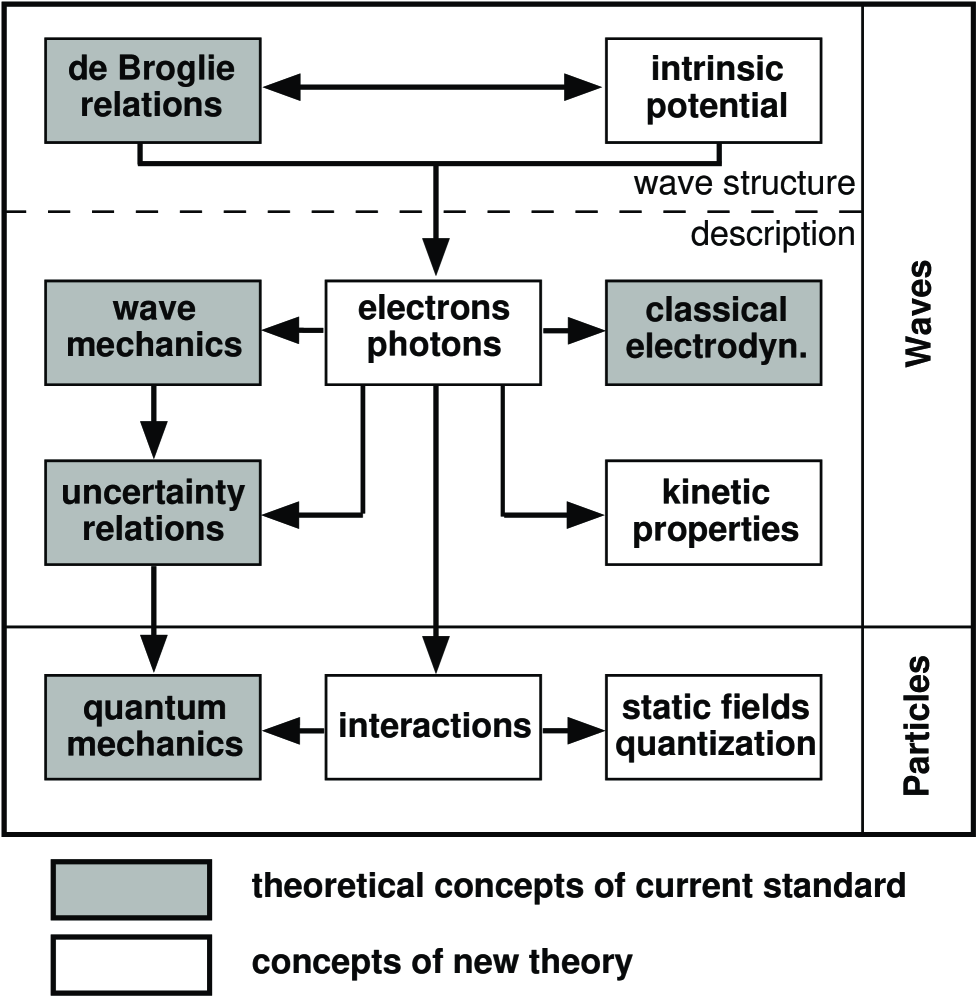
FIG. 1.: Logical structure of micro physics according to matter wave theory. Classical electrodynamics and wave mechanics describe intrinsic features of particles, quantization arises from interactions.

REFERENCES

- [1] M. Born Z. Physik 37 (1926) 863
- [2] N. Bohr ”Discussion with Einstein on Epistemological Problems in Atomic Physics”, in A. Einstein: Philosopher–Scientist, P. A. Schilpp (ed.), New York (1959)
- [3] D. Bohm Phys. Rev. 85 (1952) 166; 180
- [4] W. Heisenberg Z. Physik 43 (1927) 172
- [5] J. S. Bell Physics 1 (1964) 195
- [6] A. Aspect, J. Dalibard, and R. Roger Phys. Rev. Lett. 49 (1982) 1804
- [7] C. George, I. Prigogine, and L. Rosenfeld Mat. Fys. Medd. Dan. Vid. Selsk. 38 (12) (1972) 1
- [8] A. Einstein, N. Rosen, and B. Podolsky Phys. Rev. 47 (1935) 180
- [9] U. Röseberg in Erwin Schrödinger’s world view, J. Götschl (ed.), Kluwer, Dordrecht (1992)
- [10] L. de Broglie in his foreword to [11]
- [11] D. Bohm Causality and Chance in Modern Physics, Princeton (1957)
- [12] J. S. Bell Found. Phys. 12 (1982) 989
- [13] S. Schweber QED and the Men Who Made It, Princeton (1994)
- [14] P. A. M. Dirac Eur. J. Phys. 5 (1984) 65
- [15] L. de Broglie C.R. Acad. Sci. Paris 183 (1926) 447; 185 (1927) 580
- [16] L. de Broglie Nonlinear Wave Mechanics, Amsterdam (1960)
- [17] J. S. Bell Rev. Mod. Phys. 38 (1966) 447
- [18] P. R. Holland The Quantum Theory of Motion, Cambridge Univ. Press, Cambridge (1993)
- [19] E. Schrödinger Ann. Physik 79 (1926) 361; 489
- [20] W. Heisenberg Z. Physik 33 (1925) 879; M. Born, W. Heisenberg, and P. Jordan Z. Physik 35 (1926) 357
- [21] L. de Broglie Les Incertitudes d’Heisenberg et l’Interpretation Probabiliste de la Mecanique Ondulatoire, Gauthiers-Villars, Paris (1988)
- [22] L. de Broglie Ann. Phys. 3 (1925) 22
- [23] H. Poincare Rend. Circ. Mat. Palermo 21 (1906) 129
- [24] J. Frenkel Z. Physik 32 (1925) 518
- [25] E. C. G. Stueckelberg Comptes Rendu 207 (1938) 387
- [26] F. Bopp Ann. Physik 38 (1940) 345
- [27] A. Pais Verh. Kon. Ned. Akad. Nat. 19 (1946) 1
- [28] S. Sakata Prog. Theor. Phys. 2 (1947) 145
- [29] P. A. M. Dirac Proc. Roy. Soc. London A 167 (1938) 148
- [30] C. Davisson and L. H. Germer Phys. Rev. 30 (1927) 705
- [31] M. Planck Ann. Physik 4 (1901) 553
- [32] C. Cohen–Tannoudji, B. Diu, and F. Laloe Quantum Mechanics, Wiley & Sons, New York (1977)
- [33] W. A. Hofer Measurement processes in quantum physics: a new theory of measurements in terms of statistical ensembles, submitted (1997)
- [34] J. Jackson Classical Electrodynamics, New York (1984)
- [35] A. Einstein Ann Physik 20 (1906) 627
- [36] M. Renninger Z. Physik 136 (1953) 251
- [37] G. E. Uhlenbeck and S. A. Goudsmit Naturwiss. 13 (1925) 953; Nature 117 (1925) 264
- [38] A. Aspect PhD thesis, Universite de Paris–Sud, Centre d’ Orsay (1983)
- [39] P. Debye Phys. Zeitschr. 24 (1923) 161
- [40] A. H. Compton Phys. Rev. 22 (1923) 409