1998 26 May 1998 April 1998May 1998

Generating photon pulses with an oscillating cavity

Abstract

We study the generation of photon pulses from thermal field fluctuations through opto-mechanical coupling to a cavity with an oscillatory motion. Pulses are regularly spaced and become sharp for a high finesse cavity.

Photon production from vacuum field fluctuations reflected onto moving boundaries is now a well known phenomenon [1, 2]. For a single moving mirror motion-induced radiation is quite small since its magnitude is determined by the mirrors velocity over the speed of light while the velocity of any macroscopic mirror is restricted to the order of the sound velocity. A way to enhance the effect is to use two mirrors which form a Fabry-Pérot cavity. Motion-induced effects then take profit of resonance enhancement [3] and the number of photons radiated by the cavity is shown to approach orders of magnitude of experimental demonstrations [4]. The resonance enhancement takes place when motional photons are emitted into optical cavity modes. This occurs when the mechanical oscillation frequency is adjusted such as to be a multiple of optical resonance frequencies. Motional radiation may be interpreted as resulting from the dephasings undergone by the field as it is reflected on the moving mirrors. Inside a cavity, the field dephasings add up continously over successive reflections and may therefore become large. The total dephasing is determined by an effective velocity obtained as the product of the physical velocity with the finesse which gives roughly the number of roundtrips of a photon inside the cavity. When the effective velocity approaches the speed of light photon production concentrates in sharp pulses [5, 6, 7].

The aim of the present letter is to study the pulse shaping effect for itself. Indeed the opto-mechanical coupling between an oscillatory motion of a scatterer and field fluctuations produces a temporal redistribution of field fluctuations which leads to the emission of pulses. Here we will consider a cavity moving in thermal fluctuations. We expect this situation to allow for the observation of the pulse shaping effect in a much simpler experimental configuration than for vacuum fluctuations. Incidentally, the same computation will give the temperature which would be necessary in order to see pulse shaping for quantum vacuum.

To evaluate the motional radiation we have to evaluate the field correlation function at the output of the cavity. The main lines of the derivation are explained in detail in [7] and are not repeated here. Neglecting polarisation effects, the electromagnetic field is modelled as the sum of two scalar components counterpropagating in a two-dimensional space-time and thus defined as functions of the light cone variables $u=t-x$ and $v=t+x$ (the speed of light is set to unity). The two-dimensional model gives valid predictions in four-dimensional space-time provided that the waist of the cavity modes is much smaller than the mirrors surface. The dephasings felt by the fields as they undergo multiple reflections onto the mirrors are described by functions $f_{p}(u)$ representing the optical transformation of various input rays into a given output ray as shown in figure 1.

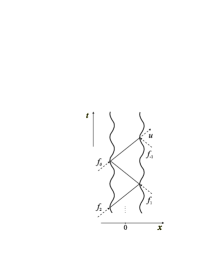
Figure 1: Space-time diagram showing the construction of the dephasings $f_{p}$ of light rays reflecting back and forth in an oscillating cavity. The oscillating lines represent the trajectories of mirrors moving in phase. The straight lines making a 45^∘light rays since the speed of light is set to unity.

For a cavity with two mirrors at rest at positions $\pm\frac{L}{2}$ those functions are simply given by $f_{p}(u)=u-pL$. The mechanical cavity length $L$ is measured as a time of flight of photons from one mirror to the other. The particular ray $f_{-1}$ represents the field directly scattered at the outer side of the cavity by the first encountered mirror. The problem of finding the functions $f_{p}$ when mirrors are moving is difficult in the general case. When large dephasings are obtained, the functions corresponding to single reflections cannot be simply added but have rather to be composed. We will use here the solution obtained in [7] for a harmonic motion which produces a very efficient opto-mechanical coupling between fields and the moving cavity.

We consider a harmonic oscillation at a frequency $\Omega=K\frac{\pi}{L}$ of order $K$ with respect to the lowest optical cavity mode. The amplitude of the mirrors motion is governed by a rapidity parameter $\alpha$ the hyperbolic tangent of which gives the maximum mechanical velocity $v={\rm th}\alpha$ normalised to the speed of light. The two mirrors are described either by the same rapidity for $K$ odd (global translation mode of the cavity) or by opposite values for $K$ even (breathing mode of the cavity). The mirrors mechanical velocity is small compared to the speed of light so that the parameter $\alpha$ is much smaller than unity. The calculation of the functions $f_{p}$ is then reduced to a composition of homographic functions and solved in an analytical manner as

$$e^{i\Omega f_{p}(u)} = \frac{a_{p}e^{i\Omega u}+b_{p}}{b_{p}^{*}e^{i\Omega u}+a_{p}^{*}}$$

$$a_{p}=(-i)^{Kp}{\rm ch}p\alpha b_{p}=i^{2K+1}(-i)^{Kp}{\rm sh}p\alpha$$ (1)

This means that the rapidity $\alpha$ adds up to $p\alpha$ under the effect of $p$ successive reflections. Mathematically this is due to the group structure of homographic functions [7]. The quantity $p\alpha$ has its order of magnitude determined by an effective rapidity

$$\alpha_{{\rm eff}}=2\frac{\alpha}{\rho}$$ (2)

where $\frac{1}{\rho}$ is the mean number of roundtrips experienced by the field before it leaves the cavity. For a high finesse cavity the effective velocity can reach large values approaching the speed of light. In fact a threshold for parametric oscillation exists at $\alpha_{{\rm eff}}=1$. At this value the energy density diverges and above threshold the system should show self-sustained oscillations. This behaviour which has been discussed in the limiting case of vanishing temperature [7] is independent of the field temperature and restricts the predictions of the present calculations to the range $\alpha_{{\rm eff}}<1$.

The energy density emitted by the cavity is then computed as the field correlation function at two coinciding points with the help of a point splitting regularization [2]. The expression for the energy density emitted by the cavity through mirror 2 is found to be

$$e_{u} = \frac{\hbar R_{2}}{48\pi}\left\{\Omega^{2}\left(f_{-1}^{\prime 2}-1\right)+\theta^{2}f_{-1}^{\prime 2}\right\}$$

$$+ \frac{\hbar T_{1}T_{2}}{48\pi}\sum_{n\geq 0}r^{2n}\left\{\Omega^{2}\left(f_{2n}^{\prime 2}-1\right)+\theta^{2}f_{2n}^{\prime 2}\right\}$$

$$+ \frac{\hbar T_{2}^{2}R_{1}}{48\pi}\sum_{n\geq 0}r^{2n}\left\{\Omega^{2}\left(f_{2n+1}^{\prime 2}-1\right)+\theta^{2}f_{2n+1}^{\prime 2}\right\}$$

$$+ \frac{\hbar T_{2}}{8\pi}\theta^{2}\sum_{n\geq 0}r^{n+1}\frac{f_{-1}^{\prime}f_{2n+1}^{\prime}}{{\rm sh}^{2}\frac{\theta}{2}(f_{-1}-f_{2n+1})}$$

$$- \frac{\hbar T_{1}T_{2}}{16\pi}\theta^{2}\sum_{n\neq m\geq 0}r^{n+m}\frac{f_{2n}^{\prime}f_{2m}^{\prime}}{{\rm sh}^{2}\frac{\theta}{2}(f_{2n}-f_{2m})}$$

$$- \frac{\hbar T_{2}^{2}R_{1}}{16\pi}\theta^{2}\sum_{n\neq m\geq 0}r^{n+m}\frac{f_{2n+1}^{\prime}f_{2m+1}^{\prime}}{{\rm sh}^{2}\frac{\theta}{2}(f_{2n+1}-f_{2m+1})}$$

$$\theta = \frac{2\pi k_{{\rm B}}T}{\hbar}\qquad r=e^{-2\rho}=\sqrt{R_{1}R_{2}}$$ (3)

The coefficient $r$ determines the attenuation factor of the field on a single cavity round-trip and can also be related to the loss parameter $\rho$. $R_{i}$ and $T_{i}$ are the reflection and transmission coefficients of the two mirrors $i=1,2$. They are related through unitarity conditions $R_{i}+T_{i}=1$. $\theta$ is the field temperature $T$ in frequency units where $k_{{\rm B}}$ is the Boltzmann constant.

The output field correlations already obtained for a cavity oscillating in quantum vacuum are recovered at the limit of vanishing temperature. In particular, the hyperbolic sine functions together with the prefactor of $\theta^{2}$ simplify to a function typical of vacuum fluctuations. In the high temperature regime $\theta\gg\Omega$ in contrast, the terms depending on hyperbolic sine functions are vanishingly small and may be ignored. A simple interpretation may therefore be proposed in this classical limit where the energy density is obtained as the result of a stretching or tightening of the energy flow lines associated with the time variation of the dephasing. The presence of additional terms at low temperature means that this classical interpretation has a restricted range of validity.

The resulting energy density emitted by the cavity as a function of time is plotted in figures 3 and 3 respectively in the low and high temperature domain. For simplicity we have supposed mirror 1 to be perfectly reflecting ($T_{1}=0$). Both figures show that pulses emerge from the cavity at regularly spaced times. The pulses are superimposed to the thermal background which is reflected back by the cavity and represents the level with respect to which they have to be distinguished. The corresponding energy density $\frac{\hbar\theta^{2}}{48\pi}$ is the same as for a motionless cavity. Figure 3 shows the result for quantum vacuum compared to fields of temperature $\theta=0.2\Omega$ and $\theta=\Omega$. It allows to evaluate the temperature which should be maintained in order to measure the pulse shaping effect due to quantum vacuum. This temperature should be of the order of $\frac{1}{10}$ of the mechanical oscillation frequency. Already at $\theta\sim\Omega$ pulse shaping would mainly be produced by the transformation of thermal photons. For a mechanical oscillation frequency of $\Omega=10$GHz, the temperature should be as low as $T=10$mK for demonstrating dissipative motional effect of vacuum.

Figure 2: Energy density emitted outside the cavity as a function of time at very low temperatures. Effective rapidity and attenuation factor are $\alpha_{{\rm eff}}=r=0.9$. The solid line corresponds to quantum vacuum, while the two other plots correspond to temperatures $\theta=0.2\Omega$ and $\theta=\Omega$.

Figure 3: Energy density emitted outside the cavity as a function of time in the high temperature domain ($\theta=3924\Omega$ corresponding to $T=300$K for $\Omega=10$GHz) for two different effective rapidities $\alpha_{{\rm eff}}=0.5$ (dashed line) and $\alpha_{\rm eff}=0.9$ (solid line). The attenuation factor is $r=0.9$. The straight line corresponds to the thermal background directly reflected by the cavity.

On the other hand, figure 3 clearly shows that pulse shaping in a thermal field is much like pulse shaping in vacuum for an oscillatory motion of the cavity. The pulses shown for two different rapidities $\alpha_{{\rm eff}}=0.5$ and $\alpha_{{\rm eff}}=0.9$ become sharper and higher when the effective rapidity is increased towards the threshold value $\alpha_{{\rm eff}}=1$. The efficiency of pulse shaping depends only on the value of the effective rapidity and not on temperature. However the orders of magnitude of the effect are much more favorable in the high temperature domain. The pulse maxima are growing in the same manner as the thermal background for increasing temperature. At the same time the number of photons per pulse increases continously. The regularly spaced radiation pulses could be more easily detected since they contain much more photons than at low temperature. If the effective rapidity is close to its threshold value the pulses emerge sufficiently from the thermal background to be distinguished.

We may get a precise idea of the order of magnitude of the motional radiation effect by evaluating the total energy in a single pulse and estimating the number of photons per pulse. To this aim, we perform the straightforward analytical integration over one oscillation period of energy density (3). To avoid lengthy expressions, we give the total energy only in the limiting case of a high cavity finesse where the orders of magnitude of pulse shaping are more favorable. We write the total emitted energy $E$ and the energy inside the cavity ${\cal E}$ for an integration time equal to a period $\frac{2\pi}{\Omega}$ of the mechanical oscillation

$$E = \frac{\hbar\theta^{2}}{12\Omega}+\frac{\hbar\Omega}{6}\frac{\rho\alpha^{2}}{\rho^{2}-\alpha^{2}}F(\theta)+\frac{\hbar\Omega}{6}\alpha^{2}(1+\theta^{2})$$

$${\cal E} = \frac{\hbar K\theta^{2}}{24\Omega}+\frac{\hbar\Omega K}{24}\frac{\alpha^{2}}{\rho^{2}-\alpha^{2}}F(\theta)$$

$$F(\theta) = 1+\frac{\theta^{2}}{\Omega^{2}}\left(1-24\sum_{l=1}^{\infty}\frac{1}{{\rm sh}^{2}(2\pi Kl\theta/\Omega)}\right)$$ (4)

The intracavity energy ${\cal E}$ is measured with respect to the Casimir energy which is the reference level obtained for a motionless cavity at zero temperature. For both expressions, the terms independent of $\alpha$ correspond to the background of thermal fluctuations integrated over one oscillation period. The other terms are proportional to $\alpha^{2}$ and therefore associated with the opto-mechanical coupling between the moving cavity and the field fluctuations. The third term in $E$ which is proportional to $\alpha^{2}$ but independent of $\rho$ describes the effect of reflection on the first encountered mirror. Evaluations in the present letter are restricted to situations below the parametric oscillation threshold $\alpha=\rho/2$. The most favorable orders of magnitude are thus obtained when $\alpha$ approaches this threshold value

$$E_{{\rm thr}} = \frac{\hbar\theta^{2}}{12\Omega}+\frac{\hbar\Omega}{18}\rho F(\theta)+\frac{\hbar\Omega}{24}\rho^{2}(1+\theta^{2})$$

$${\cal E}_{{\rm thr}} = \frac{\hbar K\theta^{2}}{24\Omega}+\frac{\hbar\Omega K}{72}F(\theta)$$ (5)

For the sake of simplicity, we may focus our attention on the high temperature limit where $F(\theta)$ has a simple quadratic dependence on temperature

$$\frac{\theta}{\Omega}\gg 1\quad\Rightarrow\quad F(\theta)\approx\frac{\theta^{2}}{\Omega^{2}}$$ (6)

Finally, the order of magnitude of the number of photons is evaluated by dividing energies by $\hbar\Omega$ and then multiplying the result by $2$ since each quantum of mechanical excitation $\Omega$ gives rise to the creation of about $2$ photons [7]. With these simplifying assumptions, we may now discuss orders of magnitude of the motional radiation effects.

In principle, the detection of the pulses should be possible by measuring the time-dependent energy density either outside or inside the cavity. Inside the cavity, motion-induced pulses may contain up to $\frac{1}{3}$ of the number of stationnary thermal photons. For an oscillation frequency of $\Omega=10$GHz and for the global translation mode $K=3$ the cavity contains more than $10^{6}$ motion-induced photons at room temperature. These photons are easily distinguishable from the background since they are gathered in sharp pulses, propagating back and forth the cavity. The energy density then reaches values as large as the background level multiplied by the cavity finesse.

The situation is less favorable for the field radiated outside the cavity. The reason is that the cavity finesse has to be chosen high enough to compensate the smallness of the oscillation velocity, at the best of the order of the sound velocity, compared to the velocity of light. As a consequence, the probability for a photon to escape from the cavity is small. This is why the ratio of motion-induced photons to background photons goes down to $\frac{2\rho}{3}$ outside the cavity. We may still take profit of the fact that they are emitted in sharp pulses to distinguish them. In fact, the contrast of pulse energy density is of the order of $1$ with respect to background energy density. Alternatively, we may discriminate motion-induced photons in the spectral domain since they are emitted at cavity resonance frequencies [7], for example at frequencies $\Omega/3,2\Omega/3,4\Omega/3,\ldots$ for the mode $K=3$, whereas background fluctuations have a standard thermal spectrum outside the cavity since they are obtained from input fluctuations through a mere reflection on the outer side of the cavity.

There remains the question whether there may be an appreciable number of motion-induced photons per pulse outside the cavity. In the high temperature limit we deduce from (5) the number of photons $N$ per pulse as a function of cavity finesse and temperature

$$\frac{\theta}{\Omega}\gg 1\quad\Rightarrow\quad N\sim\frac{\rho}{9}\frac{\theta^{2}}{\Omega^{2}}$$ (7)

The fact that energy increases as squared temperature may thus counterbalance the smallness of the cavity transmission. At room temperature each pulse may contain about $20$ motion-induced photons for $\rho=\alpha/2\sim 10^{-5}$ that is for material velocities of the order of sound velocity. Continously measuring the temporal variation of the energy density should reveal the presence of these pulses superimposed to the background.

Pulse shaping from a thermal field appears quite similar to the effect in quantum vacuum. Its efficiency is essentially the same in both cases and depends only on the effective rapidity. However, an interesting difference arises for the mode $K=1$. Photon production into this mode is suppressed by the cavity bandwidth when the cavity is moving in vacuum (cf. equation (4) for $\theta=0$). This is due to the fact that it implies photons to be emitted at frequencies close to zero which are filtered by the cavity. In a thermal field in contrast the number of photons diverges at low frequencies which counterbalances the effect of the cavity bandwidth. As a result photon production occurs for $K=1$ with the same order of magnitude than for any other mode.

Pulse shaping from field fluctuations is much more easily detectable in a thermal field than in quantum vacuum. First a single pulse contains many more photons when it is generated from a thermal field rather than from vacuum. Second the experimental setup is considerably simpler because there is no need to reach and maintain the extremely low temperatures which would be necessary to demonstrate pulse shaping from vacuum fluctuations.

References

- [1] \NameG.T. Moore \ReviewJ. Math. Phys. \Vol11 \Year1970 \Page2679
- [2] \NameS.A. Fulling \AndP.C.W. Davies \ReviewProc. R. Soc. London \VolA 348 \Year1976 \Page393
- [3] \NameM.T. Jaekel \AndS. Reynaud \ReviewJ. Physique I \Vol1 \Year1991 \Page1395
- [4] \NameA. Lambrecht, M.T. Jaekel \AndS. Reynaud \ReviewPhys. Rev. Lett. \Vol77 \Year1996 \Page615
- [5] \NameC.K. Law \ReviewPhys. Rev. Lett. \Vol73 \Year1994 \Page1931
- [6] \NameC.K. Cole \AndW.C. Schieve \ReviewPhys. Rev. \Vol52 \Year1996 \Page4405
- [7] \NameA. Lambrecht, M.T. Jaekel \AndS. Reynaud \ReviewEuropean Physical Journal \VolD \Year1998 \Pageto appear