1 Introduction

Bunching means that photons emitted by a driven system in steady state have a tendency to arrive in pairs or larger groups at a detector rather than uniformly distributed in time. More precisely, right after a photon emission the probability density for emitting another photon is larger than for a uniform distribution of corresponding emission rate. For antibunching this probability density is smaller than for a uniform distribution, and it means that the photons repel each other.

For a driven two-level system it is known that one has antibunching [1, 2, 3]. This is intuitively very simple to understand since after an emission the system is in its ground state and it requires some time to acquire enough population of the excited state for a next emission. For two independent, noninteracting, two-level atoms one also has antibunching, although not quite so pronounced as for a single atom. This was investigated experimentally in Ref. [4].

For a system of two two-level atoms with dipole-dipole interaction it is known from studies of the master or optical Bloch equations for the system that the properties of the resonance fluorescence may change considerably when compared to that for a single system [5]-[26]. In particular there is a transition from antibunching to bunching when the atomic distance becomes small and the other parameters are kept fixed (see e.g. Ref. [12]). The state space of the system is four-dimensional and the density matrices have 16 components so that the corresponding Bloch equations require diagonalization of a 16 $\times$ 16 matrix. This makes an intuitive understanding of this transition from antibunching to bunching not obvious.

It is the aim of this paper to elucidate the underlying reason and give a simple explanation for the appearance of bunching for small distances in a driven system of two two-level atoms with dipole-dipole interaction. We will trace the phenomenon to two causes. One is the form of the steady-state density matrix of the system. The other is the density matrix of the system right after an emission, called the reset matrix [27], which depends only on the state prior to the emission. In it the steady-state ground-state population has disappeared since it does not contribute to an emission, while the steady-state populations of the higher levels have been transferred to levels one step lower, in proportion to their respective decay constants, and then normalized to 1. The new populations of the intermediate states then determine the probability density for the next emission.

The transition from antibunching to bunching can be directly read off from the steady-state density matrix of the system without a lengthy calculation. For small atomic distances and for the Rabi frequency of the order of the Einstein coefficient $A$ or a few times larger the ground-state population is very large while the excited states have small but similar populations, and thus there is only a small steady-state emission rate. The large ground state population does not contribute to a photon emission and therefore disappears after an emission, while the populations of the intermediate states move to the ground state and that of the highest state to the intermediate ones, in proportion to their respective decay constants and with ensuing normalization. Hence after a photon emission the ground and excited states have suddenly acquired populations of the same order of magnitude and thus a higher emission probability density than before. This means that the photons tend to come in pairs and that there is bunching. For weaker driving and small distances the same mechanism holds. In this case the population of the ground state is even larger and that of the highest excited state smaller than for the other excited states. But its population is still large enough so that after an emission, when the populations have moved one step down, the new population of the intermediate states is larger than before so that there is an increased emission probability and thus bunching. These considerations can be applied to quite general systems.

Here we consider a system of two two-level atoms at a fixed distance $r$, interacting with the quantized radiation field and a classical laser field. Through photon exchange the radiation field mediates the $r$ dependent dipole-dipole interaction of the atoms. The dipole and rotating-wave approximation is used throughout. Retardation effects are included.

In Section 2 we briefly review the photon-counting correlation function $g(\tau)$. If $g(0)>1$ one has bunching, if $g(0)<1$ one has antibunching. In Section 3 we apply this to two two-level atoms and give an explicit expression for $g(0)$ as a function of the atomic distance and the driving field. Bunching is explicitly seen for atomic distances about a quarter of a wavelength or less.

In Section 4 we discuss the results and the simple mechanism responsible for bunching for small atomic distances. It is also made clear why an analogous argument yields antibunching for two independent non-interacting atoms and for atoms sufficiently far away.

For simplicity we consider, in the main part of the paper, coinciding atomic dipole moments and the same laser phase for each atom. In the Appendix the general case is considered, the corresponding Hamiltonian spelled out and the reset matrix given. We also outline the connection with the quantum jump approach [28, 29, 27, 30] which is equivalent to the Monte Carlo wave-function approach [31] and to quantum trajectories [32]. For a recent review of this approach see Ref. [33]. For a system of two two-level atoms with dipole-dipole interaction we carry this approach over in a form convenient for simulations .

2 Photon-counting correlation functions

We briefly review some well-known facts. As pointed out in Ref. [34] there is a minor difference between correlation functions which are based on the electric field operator and those which are based on the photon number operator. Here we employ the latter type correlation functions of second order. For simplicity we consider broad-band photon detections over all space. It is useful to distinguish clearly between correlation functions for ensembles and for a single trajectory. The latter involves a time rather than an ensemble average.

Ensemble. Consider an ensemble of laser driven atomic systems in the state $\rho$ at $t=0$ and denote by $G(t_{2},t_{1};\rho)dt_{1}dt_{2}$ the relative number of systems for which in addition to a photon in $(t_{1},t_{1}+dt_{1})$ also a photon in $(t_{2},t_{2}+dt_{2})$ is detected. If, for a particular trajectory, we denote the number of photons detected in $(t,t+\Delta t)$ by $N^{{\rm traj}}(t,t+\Delta t)$ – for small $\Delta t$ this number is either 0 or 1 – then

$$G(t_{2},t_{1};\rho)dt_{1}dt_{2}=\langle N^{{\rm traj}}(t_{1},t_{1}+dt_{1})N^{{\rm traj}}(t_{2},t_{2}+dt_{2})\rangle_{{\rm ens}}~{}.$$ (1)

Let us consider the sub-ensemble of systems which had an emission at $t_{1}$ and let us denote its normalized density matrix right after the emission by $\hat{{\cal R}}(\rho(t_{1}))$. This we call the normalized reset matrix and it will be given explicitly for a two-atom system in the next section. We denote by $I(t;\rho)$ the probability density for the emission of a photon at time $t$ (not necessarily the first photon after $t=0$) for initial density matrix $\rho$. With this one has

$$G(t_{2},t_{1};\rho)dt_{1}dt_{2}=I(t_{1};\rho)dt_{1}~{}I(t_{2}-t_{1};\hat{{\cal R}}(\rho(t_{1})))dt_{2}~{}.$$ (2)

Letting $t_{1}\rightarrow\infty$ and keeping $\tau=t_{2}-t_{1}$ fixed the first factor on the r.h.s. goes to $I_{{\rm ss}}$ and $\rho(t_{1})$ to $\rho^{{\rm ss}}$, the steady-state emission rate and density matrix, respectively. Hence

$$G(\tau)\equiv\lim_{t\rightarrow\infty}G(t+\tau,t;\rho)=I_{\rm ss}I(\tau;\hat{\cal R}(\rho^{{\rm ss}}))~{}.$$ (3)

The photon correlation function $g(\tau)$ is now defined as

$$g(\tau)\equiv~{}\frac{G(\tau)}{I_{\rm ss}I_{\rm ss}}~{}=~{}\frac{I(\tau;\hat{{\cal R}}(\rho^{\rm ss}))}{I_{\rm ss}}~{}.$$ (4)

It compares, for the steady state, the probability density for emission of a photon at a time interval $\tau$ after a preceding emission with that of a uniform distribution of emission rate $I_{ss}$.

Single trajectory. We now consider a single system with its trajectory of photon emissions and define $N^{{\rm traj}}$ as before. At instances $t_{m}^{\prime}=m\Delta t^{\prime}$ until time $T=M\Delta t^{\prime}$ one measures whether or not a photon has been emitted in $(t_{m}^{\prime},t^{\prime}_{m+1})$. Then the relative frequency of cases in which both in $(t^{\prime}_{m},t^{\prime}_{m}+\Delta t_{1})$ and $(t^{\prime}_{m}+\tau,t^{\prime}_{m}+\tau+\Delta t_{2})$ a photon has been found is given in the limit $\Delta t^{\prime}\rightarrow 0$ and $T\rightarrow\infty$, using $1/M=\Delta t^{\prime}/T$, by

$$G^{{\rm traj}}(\tau)\Delta t_{1}\Delta t_{2} = \lim_{T\to\infty}\lim_{\Delta t^{\prime}\to 0}\,{\Delta t^{\prime}\over T}\,\sum_{m}N^{\rm traj}(t_{m}^{\prime},t_{m}^{\prime}+\Delta t_{1})N^{\rm traj}(t_{m}^{\prime}+\tau,t_{m}^{\prime}+\tau+\Delta t_{2})$$ (5)

$$= \lim_{T\to\infty}\,{1\over T}\int_{0}^{T}{\rm d}t^{\prime}\,N^{\rm traj}(t^{\prime},t^{\prime}+\Delta t_{1})N^{\rm traj}(t^{\prime}+\tau,t^{\prime}+\tau+\Delta t_{2})~{}.$$

By ergodicity this should be the same for each trajectory, and therefore one can take the ensemble average of the r.h.s. without changing anything. Using Eqs. (1) and (3) one then obtains

$$G^{{\rm traj}}(\tau)=G(\tau)$$ (6)

so that both correlation functions coincide and similarly $g^{{\rm traj}}(\tau)=g(\tau)$.

We also point out the well-known fact that if one observes photons with a detector of efficiency $\eta$ less than 1 then in Eq. (4) both numerator and denominator are multiplied by $\eta$ and hence $g(\tau)$ is not affected by the detector efficiency.

One has bunching if the relative number of cases, in which shortly after emission of a photon a further photon is emitted, exceeds those for a uniform distribution of frequency $I_{\rm ss}$. Thus bunching means $g(0)>1$. Similarly one has antibunching if this number is less than for a uniform distribution, i.e. if $g(0)<1$.

3 Bunching for two atoms

We now turn to two two-level atoms with dipole-dipole interaction, driven by a laser tuned to the atomic transition frequency $\omega_{0}$. The corresponding Hamiltonian is given in the Appendix. For simplicity we consider coinciding atomic dipole moments forming an angle $\vartheta$ with the line connecting the atoms and laser radiation normal to this line so that the laser is in phase for both atoms. The Rabi frequency of the laser, denoted by $\Omega$, is then the same for both atoms. One can take $\Omega$ to be real and positive. The general case is indicated in the Appendix.

It is convenient to use the Dicke states [35] $|g\rangle=|1\rangle|1\rangle$, $|e\rangle=|2\rangle|2\rangle$, and $|s\rangle$ and $|a\rangle$ the symmetric and antisymmetric combinations of $|1\rangle|2\rangle$ and $|2\rangle|1\rangle$.

Figure 1: Dicke states and decay rates

These states play the role of dressed states for the atoms (cf. e.g. Ref. [24]), with decay constants $A\pm{\rm Re}\,C$ (see Fig.1) where $C$ is an $r$ dependent complex coupling constant. It is given for the general case in Eq. (18) of the Appendix. From Fig. 2 it is seen that $C\rightarrow 0$ for $r\rightarrow\infty$, $|$Im$|\,C\rightarrow\infty$ for $r\rightarrow 0$, while Re$\,C$ changes little with $r$. Retardation effects are included in the sense that $C$ goes to its value for a static dipole-dipole interaction when $c\rightarrow\infty$ [22].

Figure 2: Dependence of $C$ on $r$

The steady-state density matrix $\rho^{\rm ss}$ can be found from the Bloch equations [5] and is known in the literature, see e.g. Ref. [12]. One can also directly employ the Bloch equations in Eq. (24) of the Appendix and put $\dot{\rho}=\dot{\rho}^{{\rm ss}}=0$. In the Dicke basis one obtains for the diagonal elements

$$\rho^{\rm ss}_{gg}={\left(A^{2}+\Omega^{2}\right)^{2}+A^{2}\,{\rm Re}\,C\left(2A+{\rm Re}\,C\right)+A^{2}\,({\rm Im}\,C)^{2}\over N}$$

$$\rho^{\rm ss}_{ss}={\Omega^{2}\left(2A^{2}+\Omega^{2}\right)\over N}~{},~{}~{}~{}\rho^{\rm ss}_{aa}=\rho^{\rm ss}_{ee}={\Omega^{4}\over N}$$ (7)

with the normalization factor

$$N = \left(A^{2}+2\Omega^{2}\right)^{2}+A^{2}\,{\rm Re}\,C\left(2A+{\rm Re}\,C\right)+A^{2}\,({\rm Im}\,C)^{2}~{}.$$ (8)

We also need the diagonal elements of normalized reset matrix, the density matrix right after an emission. Due to an emission the populations of the excited states in the Dicke basis move down one step to lower levels in proportion to their decay constants and the previous ground-state population disappears since it does not contribute to an emission. Normalization is then achieved by dividing by the trace, tr(.). This gives

$$\langle g|\hat{\cal R}(\rho^{\rm ss})|g\rangle = \left\{(A+{\rm Re}\,C)\rho^{\rm ss}_{ss}+(A-{\rm Re}\,C)\rho^{\rm ss}_{aa}\right\}\,/\,{\rm tr(.)}$$

$$\langle s|\hat{\cal R}(\rho^{\rm ss})|s\rangle = (A+{\rm Re}\,C)\rho^{\rm ss}_{ee}\,/\,{\rm tr(.)}$$

$$\langle a|\hat{\cal R}(\rho^{\rm ss})|a\rangle = (A-{\rm Re}\,C)\rho^{\rm ss}_{ee}\,/\,{\rm tr(.)}$$ (9)

and $\langle e|\hat{\cal R}(\rho^{\rm ss})|e\rangle=0$. The complete reset matrix is given in the Appendix.

One can immediately draw the following conclusions from these expressions.
(i) For small atomic distance, $k_{0}r<2$, ${\rm Im}\,C$ and $N$ become very large. Hence, both for weak and stronger driving, the steady-state population $\rho^{\rm ss}_{gg}$ of the ground state becomes much larger than that of the excited states, and thus the steady-state emission probability is small in this case.
(ii) For strong driving, $\Omega\sim A$, the ratios of steady-state populations of the three excited states are of equal order of magnitude for all atomic distances (since Re$\,C$ does not vary much and $N$ drops out).
(iii) Right after an emission, the (large) steady-state ground-state population is discarded, the populations of $|s\rangle$ and $|a\rangle$ are transferred to $|g\rangle$ in the reset matrix and that of $|e\rangle$ to $|s\rangle$ and $|a\rangle$, all in proportion to their appropriate decay constants. Hence, after an emission and for $\Omega\sim A$, the ground-state population and that of the first excited states have become of similar magnitude (see Fig. 3 for a qualitative description).
(iv) After an emission therefore, for small atomic distance and for $\Omega\sim A$, the population of the two first excited states has increased in relation to the ground-state population. Therefore the probability density for the next photon right after an emission is higher than the steady-state emission rate. This means bunching.

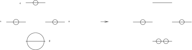
Figure 3: Relative populations before and after an emission.

This argument for bunching can be extended to weak driving and small distances as follows. From Eq. (3) one sees that in the steady state only the numerator of the ground-state population contains Im$\,C$. Since the latter increases rapidly for decreasing $r$, as seen from Fig. 2, the ratios of the populations of the excited states with that of the ground state approach 0, while the ratios among the excited states do not change. After a photon emission the upper populations move downwards and the previous large ground-state population is discarded. Hence again, after a photon emission the ratios of the populations of excited states and ground state have increased compared to the steady state if the atomic distance is sufficiently small, and this means a higher emission probability density, i.e. bunching.

These observations will now be made quantitative. Since $I_{\rm ss}$ is obtained from the level population multiplied by their decay constants $A\pm{\rm Re}\,C$, one has

$$I_{\rm ss} = (A+{\rm Re}\,C)\rho^{{\rm ss}}_{ss}+(A-{\rm Re}\,C)\rho^{{\rm ss}}_{aa}+2A\rho^{{\rm ss}}_{ee}~{}.$$ (10)

Hence the normalization constant tr(.) in Eq. (3) is $I_{\rm ss}$. For small atomic distance $I_{\rm ss}$ becomes very small, due to the small population of the excited states. This can be attributed to the detuning due to the level shift $\hbar\,{\rm Im}\,C$ (see Fig. 1).

For $g(0)$ in Eq. (4) one needs $I(0;\hat{{\cal R}}(\rho^{\rm ss}))$, the probability density for a new emission right after an emission. This is obtained in a similar way as $I_{\rm ss}$,

$$I(0;\hat{{\cal R}}(\rho^{\rm ss})) = (A+{\rm Re}\,C)\langle s|\hat{{\cal R}}(\rho^{\rm ss})|s\rangle+(A-{\rm Re}\,C)\langle a|\hat{{\cal R}}(\rho^{\rm ss})|a\rangle+2A\langle e|\hat{{\cal R}}(\rho^{\rm ss})|e\rangle$$ (11)

$$= 2\left\{A^{2}+({\rm Re}\,C)^{2}\right\}\rho^{\rm ss}_{ee}/I_{\rm ss}$$

by Eqs. (3) and (10). One could also have used Eq. (19) of the Appendix. From the behavior of Re$\,C$ it follows that $I(0;\hat{{\cal R}}(\rho^{\rm ss}))$ is of the same order of magnitude for all atomic distances. This fact is immediately understood by the observations (ii) and (iii) above. From Eqs. (4) and (3) - (11) one finally obtains

$$g(0) = {I(0;\hat{{\cal R}}(\rho^{\rm ss}))\over I_{\rm ss}}$$ (12)

$$= {A^{2}+({\rm Re}\,C)^{2}\over 2A^{2}}\,\left[\,1+{A^{2}({\rm Im}\,C)^{2}-4\Omega^{2}A{\rm Re}\,C\over\left(2\Omega^{2}+A^{2}+A{\rm Re}\,C\right)^{2}}\right]~{}.$$

Since $I_{\rm ss}$ becomes small for small $r$ while $I(0;\hat{{\cal R}}(\rho^{\rm ss})$ does not change much with $r$ one has $g(0)>1$ for small atomic distances. In the last expression the first factor approaches 1 for small atomic distance since Re$\,C$ goes to $A$, while the second factor grows with Im$\,C$.

\psfrag{D=0}{ {\tiny$\vartheta=0$}}\psfrag{D=p/4}{ {\tiny$\vartheta=\pi/4$}}\psfrag{D=p/2}{ {\tiny$\vartheta=\pi/2$}}\psfrag{a $a$}{{\tiny$k_{0}r$ \hskip 28.45274pt (a)}}\psfrag{a $b$}{{\tiny$k_{0}r$ \hskip 28.45274pt (b)}}\psfrag{g$0$}{{\tiny$g(0)$}}\epsfbox{bild29a.ps} \psfrag{D=0}{ {\tiny$\vartheta=0$}}\psfrag{D=p/4}{ {\tiny$\vartheta=\pi/4$}}\psfrag{D=p/2}{ {\tiny$\vartheta=\pi/2$}}\psfrag{a $a$}{{\tiny$k_{0}r$ \hskip 28.45274pt (a)}}\psfrag{a $b$}{{\tiny$k_{0}r$ \hskip 28.45274pt (b)}}\psfrag{g$0$}{{\tiny$g(0)$}}\epsfbox{bild29b.ps}

Figure 4: Photon correlation $g(0)$ as a function of $r$. (a) $\Omega=0.1\,A\,$, (b) $\Omega=0.9\,A$

In particular, for weak driving the terms involving $\Omega$ can be neglected and one can read off Fig. 2 that one has bunching below an atomic distance of about a quarter of the optical wavelength. For strong driving, $\Omega\sim A$, bunching sets in when the atoms are slightly closer. For large atomic distance $g(0)$ approaches $1/2$ since $C$ approaches $0$. This recovers the result for two independent atoms. This is plotted in Fig. 4.

4 Discussion

We have investigated bunching and antibunching in the resonance fluorescence of two atoms as a function of their distance and with their dipole-dipole interaction taken into account. Each atom was treated as a two-level system and the position of the atoms was kept fixed. The two-atom system was irradiated by a laser tuned to the transition frequency of the individual atoms. Retardation effects have been included.

For a single two-level atom antibunching in the resonance fluorescence is well-known and well understood [1]. After emission of a photon the atom is in its ground state and has to be pumped to the excited state before emitting a new photon. Hence the probability density for finding a second photon right after an emission is zero.

For two independent, noninteracting two level atoms one of the atoms is in its ground state right after an emission while the other is unchanged. Therefore the probability density for a second photon right after an emission is half of that in the steady state. This means $g(0)=1/2$.

For two interacting two-level atoms the emission statistics depends on the distance. For atoms far apart the interaction is negligible and one has antibunching as for two independent atoms. For small atomic distances one has bunching. The main purpose of this paper was to get a better understanding of this phenomenon.

Let $|g\rangle\equiv|1\rangle|1\rangle$ and $|e\rangle\equiv|2\rangle|2\rangle$ denote the states where both atoms are in the ground and excited state, respectively, and let $|s\rangle$ and $|a\rangle$ be the symmetric and antisymmetric combinations of $|1\rangle|2\rangle$ and $|2\rangle|1\rangle$ (Dicke states). We first discuss the case of strong driving. Then, for small distances, the steady-state ground-state population is much larger than those in $|s\rangle,|a\rangle$ and $|e\rangle$ while the populations of the latter are of similar (though small) magnitude, as indicated in Fig. 3. The reason for the small population of the latter is easily understood through the level shift of $|s\rangle$ and $|a\rangle$ due to the dipole force (see Fig. 1). The reason for the similar magnitude of the population of $|s\rangle$ and $|a\rangle$ with $|e\rangle$ has been attributed to two-photon processes connecting $|g\rangle$ with $|e\rangle$ [22]. Now, once a system has emitted a photon the population of $|e\rangle$ is transferred to $|s\rangle$ and $|a\rangle$ and the population of the two latter to $|g\rangle$, in proportion to the respective decay constants and with ensuing normalization. The previous population of $|g\rangle$ has disappeared since it does not contribute to the emission. Thus right after an emission the populations of $|s\rangle,|a\rangle$ and $|g\rangle$ are suddenly of similar magnitude while before the emission the population of the ground state was much larger. Hence right after an emission the probability density for finding another photon has increased when compared to that preceding the emission, i.e. compared to the steady state emission rate. This means bunching for small distances and strong driving.

For weak driving the mechanism is in principle the same. Although in the steady state the populations of the excited states now are no longer of similar magnitude the ground-state population increases with decreasing distance much faster than the population difference between the excited states. This means that the population of $|e\rangle$ is not too small when compared to the population of $|s\rangle$ and $|a\rangle$. Therefore after an emission, when the populations have moved down one step, the combined population of $|s\rangle$ and $|a\rangle$ has increased. This means a higher emission probability density than in the steady state, i.e. bunching.

We have shown that when decreasing the atomic distance the transition from antibunching to bunching sets in at a distance of about a quarter of the optical wavelength, for weak driving slightly sooner than for strong driving.

It is instructive to see why the same argument gives antibunching for two independent, non-interacting atoms. First, for strong driving, the two levels of each individual atom are populated by approximately $1/2$ so that the population of $|g\rangle,|s\rangle,|a\rangle$, and $|e\rangle$ are $1/4$ each. Then, after an emission, the ratios of the populations of $|g\rangle,|s\rangle$, $|a\rangle$ and $|e\rangle$ are $\frac{1}{2}~{}:~{}\frac{1}{4}~{}:~{}\frac{1}{4}~{}:~{}0$, as inherited from those of $|s\rangle,|a\rangle,|e\rangle$, prior to the emission and in proportion to the decay rates. Thus the probability density for a next emission is only one half of that in the steady state. On the other hand, for weak driving the ground-state population is much larger than that of the excited states. Is this situation not similar to that of interacting atoms? Not quite, since although the populations of $|s\rangle$ and $|a\rangle$ are small and of similar magnitude, that of $|e\rangle$ is of the order of the product of the latter and therefore an order of magnitude smaller. Thus after an emission the ground state population is still much larger than that of the excited states, and there is no increase in the emission probability.

The analysis can be carried over to the more general case where the dipole moments are not parallel and where the laser is detuned and its phase is different for the two atoms. The necessary tools are given in the Appendix. Also the case of degenerate upper level can be treated. The results [36] are similar to those obtained above.

To conclude, we have traced the appearance of bunching in the resonance fluorescence of a driven system of two two-level atoms with dipole-dipole interaction and at small distances to two causes, one the level populations of the steady-state density matrix, the other the change in the state right after the emission of a photon. A similar analysis can in principle also be applied to other systems, e.g. to a single atom in a three-level cascade configuration.

Appendix

We consider two atoms fixed at positions ${\bf r}_{i}$ and each with two levels, $|1\rangle_{i}$ and $|2\rangle_{i},i=1,2$, with energy difference $\hbar\omega_{0}$. We define operators $S^{\pm}_{i}$ in the two-atom Hilbert space by $S^{+}_{i}=|2\rangle_{ii}\langle 1|$ and $S_{i}^{-}=|1\rangle_{ii}\langle 2|$. The dipole moment of the $i$-th atom is ${\bf D}^{(i)}_{12}=~{}_{i}\langle 1|{\bf X}|2\rangle_{i}$. For the laser we take zero detuning and ${\bf E}_{L}({\bf r},t)={\rm Re}\left\{{\bf E}_{0}~{}e^{{\rm i}({\bf k}_{L}\cdot{\bf r}-\omega_{0}t)}\right\}$. Making the usual rotating-wave approximation and going over to the interaction picture the interaction Hamiltonian becomes

$$H_{\rm I}=\sum_{i=1}^{2}\sum_{{\bf k},s}\hbar\left[g_{{\bf k},s}^{(i)}a_{{\bf k},s}\,{\rm e}^{{\rm i}(\omega_{0}-\omega_{k})t}\,{\rm e}^{{\rm i}{\bf k}\cdot{\bf r}_{i}}S_{i}^{+}+\,{\rm h.c.}\,\right]+H_{L}~{},$$ (13)

with the coupling constants

$$g_{{\bf k},s}^{(i)} = {\rm i}e\left({\omega_{k}\over 2\epsilon_{0}\hbar L^{3}}\right)^{1/2}\left({\bf D}^{(i)}_{12},{\bf\epsilon}_{{\bf k},s}\right),$$ (14)

laser part $H_{L}=~{}\frac{\hbar}{2}~{}\sum^{2}_{i=1}\left\{\Omega_{i}S_{i}^{+}+\Omega_{i}^{\star}S_{i}^{-}\right\}$ and Rabi frequencies $\Omega_{i}=~{}\frac{e}{\hbar}~{}{\bf D}_{12}^{(i)}\cdot{\bf E}_{0}~{}e^{i{\bf k}_{L}\cdot{\bf r}_{i}}$. The operator $H_{I}$ contains the dipole-dipole interaction of the two atoms as seen from the Bloch equations or from the conditional Hamiltonian between emissions, as explained further below. In the above Power-Zienau formulation this interaction is due to photon exchange [5].

Reset matrix. The reset operation gives the state or density matrix right after a photon detection. In a basis in which the atomic damping is diagonal, as for the Dicke states, the diagonal states immediately can be written down, as in Eq. (3). For a general $N$-level system the reset matrix has been derived in Refs. [27, 30]. For a system consisting of two or more atoms the derivation has to slightly modified since in this case the field operator ${\bf E}$ appear with different position arguments.

Let at time $t$ the state of the combined system, atoms plus quantized radiation field, be given by $|0_{\rm ph}\rangle\,\rho\,\langle 0_{\rm ph}|$, i.e. the atomic system is described by the density matrix $\rho$ and there are no photons (recall that the laser field is treated classically). If at time $t+\Delta t$ a photon is detected (but not absorbed) the combined system is in the state

$$I\!\!P_{\!>}U_{I}(t+\Delta t,t)|0_{\rm ph}\rangle\,\rho\,\langle 0_{\rm ph}|U_{I}^{\dagger}(t+\Delta t,t)I\!\!P_{\!>}$$ (15)

where $I\!\!P_{\!>}={\bf 1}-|0_{\rm ph}\rangle{\bf 1}_{A}\langle 0_{\rm ph}|$ is the projector onto the one or more photon space (since $\Delta t$ is small one could directly take the projector onto the one-photon space). The probability for this event is the trace over Eq. (15). For the state of the atomic system it is irrelevant whether the detected photon is absorbed or not (intuitively the photon travels away and does no longer interact with the atomic system). Hence after a photon detection at time $t+\Delta t$ the non-normalized state of the atomic system alone, denoted by ${\cal R}(\rho)\Delta t$, is given by a partial trace over the photon space,

$${\cal R}(\rho)\Delta t={\rm tr_{ph}}\left(I\!\!P_{\!>}U_{I}(t+\Delta t,t)|0_{ph}\rangle\,\rho\,\langle 0_{ph}|U^{\dagger}_{I}(t+\Delta t,t)I\!\!P_{\!>}\right)~{}.$$ (16)

We call ${\cal R}(\rho)$ the non-normalized reset state [27]. Proceeding as in Refs. [27, 30] and using perturbation theory one obtains [36]

$${\cal R}(\rho) = {1\over 2}\left(C_{12}^{*}+C_{21}\right)S_{1}^{-}\rho S_{2}^{+}+{1\over 2}\left(C_{12}+C_{21}^{*}\right)S_{2}^{-}\rho S_{1}^{+}$$ (17)

$$+A\left(S_{1}^{-}\rho S_{1}^{+}+S_{2}^{-}\rho S_{2}^{+}\right)$$

with the $r$ dependent constants

$$C_{ij} = {3A\over 2}\,{\rm e}^{{\rm i}k_{0}r}\Bigg{[}{1\over{\rm i}k_{0}r}\left(\left(\hat{{\bf D}}_{12}^{(i)},\hat{{\bf D}}_{12}^{(j)}\right)-\left(\hat{{\bf D}}_{12}^{(i)},\hat{{\bf r}}\right)\left(\hat{{\bf r}},\hat{{\bf D}}_{12}^{(j)}\right)\right)$$ (18)

$$+\left({1\over(k_{0}r)^{2}}-{1\over{\rm i}(k_{0}r)^{3}}\right)\left(\left(\hat{{\bf D}}_{12}^{(i)},\hat{{\bf D}}_{12}^{(j)}\right)-3\left(\hat{{\bf D}}_{12}^{(i)},\hat{{\bf r}}\right)\left(\hat{{\bf r}},\hat{{\bf D}}_{12}^{(j)}\right)\right)\Bigg{]}~{}.$$

Here $\hat{~{}}$ denotes vectors normalized to 1, A is the Einstein coefficient, and ${\bf r}={\bf r}_{2}-{\bf r}_{1}$. In the case of equal dipole moments one has $C_{12}=C_{21}\equiv C$ which was depicted in Fig. 2, with $\vartheta$ defined by $\cos^{2}\vartheta=\left|\left({\bf D}_{12},{\bf r}\right)\right|^{2}/r^{2}D_{12}^{2}$. The normalized reset state is $\hat{{\cal R}}(\rho)\equiv{\cal R}(\rho)/{\rm tr}{\cal R}(\rho)$.

By Eq. (15) the normalization of ${\cal R}(\rho)$ is such that tr${}_{A}{\cal R}(\rho)\Delta t$ is the probability for a photon detection at time $t+\Delta t$ if the (normalized) state of the atomic system at time $t$ is $\rho$. Hence one has for the probability density $I$ of Section 2

$$I(t;\rho(0))={\rm tr}\,{\cal R}(\rho(t))~{}.$$ (19)

The laser field does not appear in the reset state, just as in the case of a single atom [27, 30], since its effect during the short time $\Delta t$ is negligible. By a simple calculation one checks that Eq. (17) can be written as

$${\cal R}(\rho)=\left(A+~{}\frac{1}{2}~{}|C_{12}+C^{\star}_{21}|\right)R_{+}\rho R^{\dagger}_{+}+\left(A-~{}\frac{1}{2}~{}|C_{12}+C_{21}^{\star}|\right)R_{-}\rho R_{-}^{\dagger}$$ (20)

where $R_{\pm}=\left(S_{1}^{-}\pm e^{i\varphi}S_{2}^{-}\right)/\sqrt{2}$ and $\varphi$ is the argument of $C_{12}+C_{12}^{\star}$. From Eq. (18) one can check that $A\geq\frac{1}{2}|C_{12}+C_{21}^{\star}|$. If $\rho$ is a pure state, $\rho=|\psi\rangle\langle\psi|$ say, then $R_{\pm}\rho R_{\pm}^{\dagger}$ are also pure states. This decomposition of ${\cal R}(\rho)$ is advantageous for simulations of trajectories.

Conditional Hamiltonian and waiting times. In the quantum jump approach [28, 29, 27, 33], the time development of an atomic system is described by a conditional non-hermitian Hamiltonian $H_{{\rm cond}}$, which gives the time development between photon emissions, and by a reset operation which gives the state or density matrix right after an emission. For a general $N$-level system these have been derived in Refs. [27, 30]. The derivation of the former is adapted here to a system of two atoms.

As explained in Refs. [28, 27, 30, 33], $H_{{\rm cond}}$ is of the general form $H_{{\rm cond}}=H_{A}+H_{L}+\Gamma$ where $\Gamma$ is an atomic damping operator. In a basis in which $\Gamma$ is diagonal the diagonal terms are just the decay constants of the corresponding states. If these (dressed) states are known $H_{{\rm cond}}$ can immediately be written down. In this way one can obtain $H_{{\rm cond}}$ for parallel dipole moments in the Dicke basis. In the general case it is obtained (in the interaction picture) from the short-time development under the condition of no emission, i.e. from the relation

$${\bf 1}-~{}\frac{\rm i}{\hbar}~{}H_{{\rm cond}}\Delta t=\langle 0_{ph}|U_{I}(\Delta t,0)|0_{ph}\rangle$$

where the r.h.s. is evaluated in second order perturbation theory for $\Delta t$ intermediate between inverse optical frequencies and atomic decay times. In a similar way as for a single atom [28, 27, 30] one obtains for two two-level atoms [36]

$$H_{\rm cond} = \frac{\hbar}{2{\rm i}}\left[A\left(S_{1}^{+}S_{1}^{-}+S_{2}^{+}S_{2}^{-}\right)+C_{12}\,S_{1}^{+}S_{2}^{-}+C_{21}\,S_{2}^{+}S_{1}^{-}\right]+H_{L}$$ (21)

with the $r$ dependent constant $C_{ij}$ given by Eq. (18). Between emissions the time development is given by $U_{{\rm cond}}(t,0)=\exp\left\{-{\rm i}H_{{\rm cond}}t/\hbar\right\}$ which is non-unitary since $H_{{\rm cond}}$ is non-hermitian. The corresponding decrease in the norm of a vector is connected to the waiting time [37] for emission of a (next) photon. If at $t=0$ the initial atomic state is $|\psi\rangle$ then the probability $P_{0}(t)$ to observe no photon until time $t$ by a broadband counter (over all space) is given by [28, 27, 30]

$$P_{0}(t;|\psi\rangle)=\|U_{{\rm cond}}(t,0)|\psi\rangle\|^{2}~{},$$ (22)

and the probability density $w_{1}$ of finding the first photon at time $t$ is

$$w_{1}(t;|\psi\rangle)=-~{}\frac{d}{dt}~{}P_{0}(t;|\psi\rangle)~{}.$$ (23)

For an initial density matrix instead of $|\psi\rangle$ the expressions are analogous, with a trace instead of a norm squared in Eq. (22). For $t=0$ one must have $w_{1}(0)=I(0)$ since for short times any photon must be the first. This identity is easily checked by means of Eqs. (22), (19) and (17).

For equal dipole moments and without laser the conditional Hamiltonian is diagonal in the Dicke basis. $A\pm{\rm Re}\,C$ describes the decay rates of $|s\rangle$ and $|a\rangle$ to $|g\rangle$, while $\pm\hbar~{}{\rm Im}\,C$ can be viewed as a level shift. The state $|e\rangle$ can decay to both $|s\rangle$ and $|a\rangle$, with respective decay rates $A\pm{\rm Re}\,C$. This also follows from the Bloch equations and is indicated in Fig. 1. From this the well-known fact follows that two atoms with dipole interaction can decay faster or slower than two independent atoms (super- and sub-radiance [25]). When $r\rightarrow 0$, ${\rm Re}\,C$ approaches $A$ so that $|a\rangle$ can no longer decay while $|s\rangle$ decays with $2A.$

Trajectories and Bloch equations. Starting at $t=0$ with a pure state, the state develops according to $U_{{\rm cond}}$ until the first emission at some time $t_{1}$, determined from $w_{1}$ in Eq. (23). Then the state is reset according to Eq. (17) to a new density matrix (which has to be normalized), and so on.

The decomposition of ${\cal R}(\rho)$ in Eq. (20) allows one, however, to work solely with pure states which is numerically much more efficient. One can start with a pure state $|\psi\rangle$, develop it with $U_{{\rm cond}}$ until $t_{1}$ to the (non-normalized) $|\psi(t_{1})\rangle$, reset to one of the pure states $R_{\pm}|\psi(t_{1})\rangle/\|\cdot\|$ with relative probabilities given by the factors $A\pm~{}\frac{1}{2}|C_{12}+C_{21}^{\star}|$ appearing in Eq. (20), and so on. The waiting time distributions are not changed by this procedure.

Quite generally the ensemble of such trajectories yields the Bloch equations [27]. With the reset matrix this is easily seen as follows. If an ensemble of systems of two two-level atoms has a density matrix $\rho(t)$ at time $t$ then at time $t+\Delta t$ one has two sub-ensembles, one with a photon emission, the other with none. The former has relative size tr$\,{\cal R}(\rho(t))\Delta t$, by the remark after Eq. (17), while the latter is obtained by means of $U_{{\rm cond}}(t+\Delta t,t)={\bf 1}_{A}-~{}\frac{i}{\hbar}H_{{\rm cond}}\Delta t$. This immediately gives

$$\dot{\rho}=-~{}\frac{\rm i}{\hbar}~{}[H_{{\rm cond}}\rho-\rho H^{\dagger}_{{\rm cond}}]+{\cal R}(\rho)~{}.$$ (24)

Inserting from Eqs. (21) and (17) one obtains the Bloch equations for two two-level atoms. They agree with those derived by Agarwal [5]. From this expression it is evident that $H_{\rm cond}$ or the reset matrix can be immediately determined if the Bloch equations and the reset matrix or, respectively, $H_{\rm cond}$ are explicitly known.

References

- [1] H. J. Carmichael and D. F. Walls, J. Phys. B 9, L43 (1976); J. Phys. B 9, 1199 (1976)
- [2] H. J. Kimble, M. Dagenais, and L. Mandel, Phys. Rev. Lett. 39, 691 (1977)
- [3] F. Diedrich and H. Walther, Phys. Rev. Lett. 58, 203 (1987)
- [4] W. M. Itano, J. C. Berquist and D. J. Wineland, Phys. Rev. A 38, 559 (1988)
- [5] G. S. Agarwal, Quantum Optics, Springer Tracts of Modern Physics Vol. 70 (Springer-Verlag, Berlin 1974)
- [6] G. S. Agarwal, A. C. Brown, L. M. Narducci, and G. Vetri, Phys. Rev. A 15, 1613 (1977)
- [7] I. R. Senitski, Phys. Rev. Lett. 40, 1334 (1978)
- [8] H. S. Freedhoff, Phys. Rev. A 19, 1132 (1979)
- [9] G. S. Agarwal, R. Saxena, L. M. Narducci, D. H. Feng, and R. Gilmore, Phys. Rev. A 21, 257 (1980)
- [10] G. S. Agarwal, L. M. Narducci, and E. Apostolidis, Opt. Commun. 36, 285 (1981)
- [11] M. Kus and K. Wodkiewicz, Phys. Rev. A 23, 853 (1981)
- [12] Z. Ficek, R. Tanas and S. Kielich, Opt. Acta 30, 713 (1983)
- [13] Z. Ficek, R. Tanas and S. Kielich, Opt. Acta 33, 1149 (1986)
- [14] J.F. Lam and C. Rand, Phys. Rev. A 35, 2164 (1987)
- [15] Z. Ficek, R. Tanas and S. Kielich, J. Mod. Opt. 35, 81 (1988)
- [16] B. H. W. Hendriks and G. Nienhus, J. Mod. Opt. 35, 1331 (1988)
- [17] M. S. Kim, F. A. M. Oliveira, P. L. Knight, Opt. Commun. 70, 473 (1989)
- [18] S. V. Lawande, B. N. Jagatap and Q. V. Lawande, Opt. Comm. 73, 126 (1989)
- [19] Q. V. Lawande, B. N. Jagatap and S. V. Lawande, Phys. Rev. A 42, 4343 (1990)
- [20] Z. Ficek and B.C. Sanders, Phys. Rev. A 41, 359 (1990)
- [21] K. Yamada and P. R. Berman, Phys. Rev. A 41, 453 (1990)
- [22] G. V. Varada and G. S. Agarwal, Phys. Rev. A 45, 6721 (1992)
- [23] D. F. V. James, Phys. Rev. A 47, 1336 (1993)
- [24] R. G. Brewer, Phys. Rev. A 52, 2965 (1995), Phys. Rev. A 53, 2903 (1996)
- [25] R. G. DeVoe and R. G. Brewer, Phys. Rev. Lett. 76, 2049 (1996)
- [26] P. R. Berman, Phys. Rev. A 50, 4466 (1997)
- [27] G. C. Hegerfeldt, Phys. Rev. A 47, 449 (1993)
- [28] G. C. Hegerfeldt and T. S. Wilser, in: Classical and Quantum Systems. Proceedings of the II. International Wigner Symposium, July 1991, edited by H. D. Doebner, W. Scherer, and F. Schroeck; World Scientific (Singapore 1992), p. 104
- [29] T. Wilser, Doctoral Dissertation, Universit t Göttingen (1991)
- [30] G. C. Hegerfeldt and D. G. Sondermann, Quantum Semiclass. Opt. 8, 121 (1996)
- [31] J. Dalibard, Y. Castin, and K. Mølmer, Phys. Rev. Lett. 68, 580 (1992)
- [32] H. Carmichael, An Open Systems Approach to Quantum Optics, Lecture Notes in Physics m 18, Springer (Berlin 1993)
- [33] M. B. Plenio and P. L. Knight, Rev. Mod. Phys. 70, 1010 (1998)
- [34] L. Mandel and E. Wolf, Optical coherence and quantum optics, Cambridge University Press 1995
- [35] R. H. Dicke, Phys. Rev. 93, 99 (1954)
- [36] A. Beige, Doctoral Dissertation, Universit t G ttingen (1997)
- [37] C. Cohen-Tannoudji and J. Dalibard, Europhys. Lett. 1, 441 (1986)