Stochastic wave function approach to generalized master equations

Abstract

A generalization of the stochastic wave function method is presented which allows the unravelling of arbitrary linear quantum master equations which are not necessarily in Lindblad form and, moreover, the explicit treatment of memory effects by employing the time-convolutionless projection operator technique. The crucial point of this construction is the description of the open system in a doubled Hilbert space, which has already been successfully used for the computation of multitime correlation functions.

I Introduction

Usually, the state of an open quantum system is described by a reduced density matrix $\rho(t)$ which is a positive operator on the Hilbert space ${\cal H}_{\rm S}$ of the system. On the other hand, within the stochastic wave function method the state of the open system is described by an ensemble of pure, normalized states $\psi(t)$ the covariance matrix of which equals the reduced density matrix [2, 3, 4, 5, 6],

$$\rho(t)=\int D\psi D\psi^{*}|\psi\rangle\langle\psi|P[\psi,t].$$ (1)

In Eq. (1) the integral extends over the Hilbert space of the system, $D\psi D\psi^{*}$ denotes the Hilbert space volume element, and $P[\psi,t]$ is the time-dependent probability density of finding the state of the system in the volume element $D\psi D\psi^{*}$ near $\psi$ [6]. This formulation has essentially two advantages compared to the conventional description: First, this approach allows the investigation of the dynamics of an individual quantum system which is continuously observed by some measurement device [7, 8], whereas the reduced density matrix can only describe the state of an ensembles of quantum systems. Second, from a computational point of view, the numerical integration of the quantum master equation can become rather expensive for large systems, since the reduced density matrix has $N^{2}$ degrees of freedom, where $N$ is the dimension of the system’s Hilbert space. In contrast, a stochastic wave function has only $N$ components, which can significantly reduce the computational expense [9]. Moreover, algorithms which are based on stochastic simulations can easily be implemented on parallel computers.

The dynamics of the stochastic wave function is governed by a stochastic evolution equation, and the construction of this evolution equation within the Born-Markov approximation is well understood. However, in some situations non-Markovian effects can significantly alter the reduced system dynamics. In this article we will present a scheme which allows a systematic incorporation of memory effects into the stochastic wave function method. To this end, we make use of an expansion scheme which is known from the theory of non-equilibrium statistical mechanics – the time-convolutionless projection operator technique [10, 11].

This article is organized as follows. In Sec. II we discuss the unravelling of quantum master equations by stochastic wave functions. This concept is well known for quantum master equations which are in Lindblad form [12] and we briefly summarize the major results in Sec. II A. In Sec. II B we generalize this concept to the treatment of arbitrary linear quantum master equations. Using this result, we present in Sec. III a general framework which allows an explicit treatment of memory effects within the stochastic wave function method. This concept is then illustrated by means of an exactly solvable model in Sec. IV – the damped Jaynes-Cummings model.

II Stochastic simulation of quantum master equations

A Quantum master equations in Lindblad form

In the Markovian regime, the time evolution of the reduced density matrix $\rho(t)$ is governed by the quantum master equation in Lindblad form

$$\frac{\partial}{\partial t}\rho(t)=-i\left[H_{\rm S}+\frac{1}{2}\sum_{i}S_{i}(t)L_{i}^{\dagger}L_{i},\rho(t)\right]$$ (2)

$$+ \sum_{i}\gamma_{i}(t)\left\{-\frac{1}{2}L_{i}^{\dagger}L_{i}\rho(t)-\frac{1}{2}\rho(t)L_{i}^{\dagger}L_{i}+L_{i}\rho(t)L_{i}^{\dagger}\right\},$$ (3)

where $H_{\rm S}$ is the Hamiltoninan of the system, the time-dependent coefficients $S_{i}(t)$ describe an energy shift induced by the coupling to the environment, namely the Lamb and Stark shifts, and the positive rates $\gamma_{i}(t)$ model the dissipative coupling to the $i-$th decay channel. This evolution equation is either obtained by a phenomenological ansatz or through a derivation which is based on a microscopic model of the system-reservoir interaction.

Using similar techniques, one can also obtain a Markovian time evolution equation for the stochastic state vector $\psi$. There are several phenomenological approaches which simply construct a stochastic evolution equation in such a way, that the equation of motion of the covariance matrix is the quantum master equation [3, 4, 5]. This procedure is often called unravelling of the quantum master equation [2]. Other approaches are based on a continuous observation of the system under consideration by some measurement device, for example a photon detector, and employ the basic measurement postulates for the description of the dynamics of an individual quantum system [7, 8]. Finally, similar to the derivation of the quantum master equation, it is also possible to obtain the stochastic time evolution directly from an underlying microscopic model by an explicit derivation of the differential Chapman Kolmogorov equation for the probability density $P[\psi,t]$ [6].

A particular example of such a stochastic evolution equation which arises in the above approaches is the stochastic differential equation

$$d\psi(t)=-iG(\psi,t)dt+\sum_{i}\left(\frac{L_{i}\psi(t)}{\|L_{i}\psi(t)\|}-\psi(t)\right)dN_{i}(t),$$ (4)

where the $dN_{i}(t)$ are the differentials of independent Poisson process $N_{i}(t)$ with mean $\langle dN_{i}(t)\rangle=\gamma_{i}(t)\|L_{i}\psi(t)\|^{2}dt$ and

$$G(\psi,t) = H(t)\psi+\frac{1}{2}\sum_{i}S_{i}(t)L_{i}^{\dagger}L_{i}\psi$$ (6)

$$-\frac{i}{2}\sum_{i}\gamma_{i}(t)\left(L_{i}^{\dagger}L_{i}-\|L_{i}\psi\|^{2}\right)\psi.$$

This particular equation of motion describes the time evolution of a piecewise deterministic process. The differential of the Poisson process $dN_{i}(t)$ can either take the value $0$ or $1$. If $dN_{i}(t)=0$, then the system evolves continuously according to the nonlinear Schrödinger-type equation

$$i\frac{\partial}{\partial t}\psi(t)=G(\psi,t),$$ (7)

whereas, if $dN_{i}(t)=1$ for some $i$, then the system undergoes an instantaneous, discontinuous transition of the form

$$\psi(t)\longrightarrow\frac{L_{i}\psi(t)}{\|L_{i}\psi(t)\|}.$$ (8)

Note that the generator $G(\psi,t)$ of the continuous time evolution is non-Hermitian and hence the propagator of $\psi(t)$ is non-unitary. However, due to the nonlinearity of the generator, the norm of $\psi(t)$ is preserved in time.

Using the standard Ito calculus for the differentials $dN_{i}(t)$ of a Poisson process, i. e., $dN_{i}(t)dN_{j}(t)=\delta_{ij}dN_{i}(t)$, it is easy to check, that the equation of motion of the covariance matrix of $\psi(t)$ equals the usual Markovian quantum master equation for the reduced density matrix in Lindblad form. Thus, both descriptions yield the same equations of motion for the expectation values of system observables. Finally, we want to remark that it is also possible to extend the stochastic wave functions method to the calculation of arbitrary matrix elements of system operators and hence to the determination of multitime correlation functions [5, 13].

B General quantum master equations

In this section we present a generalization of the stochastic wave function method to quantum master equations which are not in Lindblad form (in Sec. III we will also encounter this type of evolution equations). To be more specific, we consider an equation of motion for the reduced density matrix of the form

$$\frac{\partial}{\partial t}\rho(t)=A(t)\rho(t)+\rho(t)B^{\dagger}(t)+\sum_{i}C_{i}(t)\rho(t)D_{i}^{\dagger}(t),$$ (9)

with some arbitrary time-dependent linear operators $A(t)$, $B(t)$, $C_{i}(t)$, and $D_{i}(t)$. This form represents the most general linear equation of motion for $\rho(t)$, which is local in time, i. e., an equation of motion where $\dot{\rho}(t)$ only depends on $\rho(t)$. In order to find an unravelling of this equation of motion we follow a strategy, which has already been successfully applied to the calculation of multitime correlation functions [13]: We describe the state of the open system by a pair of stochastic state vectors $\theta=(\phi,\psi)^{T}$ which is an element of the doubled Hilbert space $\widetilde{\cal H}={\cal H}\oplus{\cal H}$, in such a way, that

$$\rho(t)=\int D\theta D\theta^{*}|\phi\rangle\langle\psi|\widetilde{P}[\theta,t],$$ (10)

where the integral extends over the doubled Hilbert space $\widetilde{\cal H}$, and $\widetilde{P}[\theta,t]$ is the probability density of finding the system in the “state” $\theta$ at time $t$. Furthermore, we define the operators $F(t)$ and $J_{i}(t)$ as

$$F(t)=\left(\begin{array}[]{cc}A(t)&0\\ 0&B(t)\end{array}\right),\quad J_{i}(t)=\left(\begin{array}[]{cc}C_{i}(t)&0\\ 0&D_{i}(t)\end{array}\right).$$ (11)

An unravelling of the quantum master equation (9) by a stochastic wave function $\theta(t)$ can be obtained using the stochastic differential equation

$$d\theta(t) = -iG(\theta,t)dt$$ (13)

$$+\sum_{i}\left(\frac{\|\theta(t)\|}{\left\|J_{i}(t)\theta(t)\right\|}J_{i}(t)\theta(t)-\theta(t)\right)dN_{i}(t),$$

where $dN_{i}(t)$ is the differential of a Poisson process with mean

$$\langle dN_{i}(t)\rangle=\frac{\left\|J_{i}(t)\theta(t)\right\|^{2}}{\|\theta(t)\|^{2}}dt,$$ (14)

and

$$G(\theta,t)=i\left(F(t)+\frac{1}{2}\sum_{i}\frac{\left\|J_{i}(t)\theta(t)\right\|^{2}}{\|\theta(t)\|^{2}}\right)\theta(t).$$ (15)

Again, the stochastic differential equation (13) describes a piecewise deterministic jump process, where $G(\theta,t)$ is the generator of the continuous time evolution and the operators $J_{i}(t)$ lead to discontinuous instantaneous transitions. In order to show that the stochastic differential equation (13) leads to the correct equation of motion for $\rho(t)$ one can rewrite Eq. (13) as a system of coupled stochastic differential equations for $\phi$ and $\psi$, and compute the mean of the differential

$$d\left(|\phi\rangle\langle\psi|\right)=|d\phi\rangle\langle\psi|+|\phi\rangle\langle d\psi|+|d\phi\rangle\langle d\psi|$$ (16)

using the Ito calculus, which justifies our ansatz. It is important to note that this unravelling also contains the unravelling presented in Sec. II A. If the equation of motion for the reduced density matrix is in Lindblad form, and $\phi(0)=\psi(0)$ then it is easy to see that $\phi(t)$ and $\psi(t)$ are identical for all $t$ and the stochastic differential equation (13) reduces to Eq. (4) with the choice

$$A(t)=B(t)=-iH_{\rm S}-\frac{1}{2}\sum_{k}\left[\gamma_{k}(t)+iS_{k}(t)\right]L_{k}^{\dagger}L_{k}$$ (17)

and

$$C_{i}(t)=D_{i}(t)=\sqrt{\gamma(t)}L_{i}.$$ (18)

III Non-Markovian stochastic wave function method

In this section we present a general scheme which allows a systematic, perturbative treatment of memory effects within the stochastic wave function method. This approach is based on the time-convolutionless projection operator technique [10, 11], which is related to the Nakajima-Zwanzig projection operator technique [14, 15, 16].

As a microscopic model, we consider a system which is coupled to an environment. The Hamiltonian of the total system is given by

$$H=H_{0}+\alpha H_{\rm I},$$ (19)

where $H_{0}$ describes the free evolution of the system and the reservoir and $H_{\rm I}$ their interaction. The parameter $\alpha$ denotes a dimensionless expansion parameter. The state of the total system is described by the interaction picture density matrix $W(t)$ which is a solution of the Liouville-von Neumann equation

$$\frac{\partial}{\partial t}W(t)=-i\alpha[H_{\rm I}(t),W(t)]\equiv\alpha L(t)W(t),$$ (20)

where the interaction Hamiltonian in the interaction picture is defined as $H_{\rm I}(t)=\exp(iH_{0}t)H_{\rm I}\exp(-iH_{0}t)$. Since we are interested in the dynamics of the reduced system, we define a projector ${\cal P}$ as

$${\cal P}W(t)=\mbox{Tr}_{\rm R}\left\{W(t)\right\}\otimes\rho_{\rm R}\equiv\rho(t)\otimes\rho_{\rm R},$$ (21)

where $\rho_{\rm R}$ is a stationary state of the environment, and a projector ${\cal Q}=1-{\cal P}$. A quasi-closed equation of motion for ${\cal P}W(t)$ can be obtained by using the Nakajima-Zwanzig projection operator technique [14, 15, 16], namely

$$\frac{\partial}{\partial t}{\cal P}W(t)=\int_{0}^{t}ds\widetilde{K}(t,s){\cal P}W(s),$$ (22)

where the memory kernel $\widetilde{K}(t,s)$ is defined as

$$\widetilde{K}(t,s)=\alpha^{2}{\cal P}L(t){\cal G}(t,s)L(s),$$ (23)

with the propagator

$${\cal G}(t,s)={\rm T}_{\leftarrow}\exp\left[\alpha\int_{s}^{t}ds^{\prime}{\cal Q}L(s^{\prime})\right]$$ (24)

and ${\rm T}_{\leftarrow}$ indicates the chronological time ordering. In obtaining Eq. (22) we have assumed that $\mbox{Tr}_{\rm R}\{H_{\rm I}^{2k+1}\rho_{\rm R}\}=0$, and that the system and the reservoir are uncorrelated initially, i. e., $W(0)=\rho(0)\otimes\rho_{\rm R}$. To eliminate the time-convolution [10, 11] in Eq. (22) we replace $W(s)$ by the expression

$$W(s)=G(t,s)({\cal P}+{\cal Q})W(t),$$ (25)

where the backward propagator $G(t,s)$ is defined as

$$G(t,s)={\rm T}_{\rightarrow}\exp\left[-\alpha\int_{s}^{t}ds^{\prime}L(s^{\prime})\right]$$ (26)

and ${\rm T}_{\rightarrow}$ indicates the anti-chronological time ordering. This leads to the time-convolutionless equation of motion

$$\frac{\partial}{\partial t}{\cal P}W(t)=K(t){\cal P}W(t),$$ (27)

where the generator $K(t)$ is defined as

$$K(t)=\alpha{\cal P}L(t)[1-\Sigma(t)]^{-1}{\cal P}$$ (28)

and

$$\Sigma(t)=\alpha\int_{0}^{t}ds{\cal G}(t,s)L(s){\cal P}G(t,s).$$ (29)

If the operator $(1-\Sigma(t))^{-1}$ can be expanded in a geometric series, which is possible if the coupling between the system and the reservoir is not too strong, then we can rewrite the generator $K(t)$ as

$$K(t)=\alpha\sum_{n=0}^{\infty}{\cal P}L(t)\left(\Sigma(t)\right)^{n}{\cal P}$$ (30)

and obtain a perturbative expansion in the form

$$K(t)=\sum_{n=0}^{\infty}\alpha^{2n}K_{2n}(t).$$ (31)

Note that all terms containing odd orders of the coupling constants vanish, since by definition of ${\cal P}$ and $L(t)$ we have ${\cal P}L(t_{1})\cdots L(t_{2k+1}){\cal P}=0$. The explicit expressions for the second and fourth order contribution are

$$K_{2}(t)=\int_{0}^{t}dt_{1}{\cal P}L(t)L(t_{1}){\cal P},$$ (32)

and

$$K_{4}(t)=\int_{0}^{t}dt_{1}\int_{0}^{t_{1}}dt_{2}\int_{0}^{t_{2}}dt_{3}$$ (35)

$$\times\Big{[}{\cal P}L(t)L(t_{1})L(t_{2})L(t_{3}){\cal P}-{\cal P}L(t)L(t_{1}){\cal P}L(t_{2})L(t_{3}){\cal P}$$

$$-{\cal P}L(t)L(t_{2}){\cal P}L(t_{1})L(t_{3}){\cal P}-{\cal P}L(t)L(t_{3}){\cal P}L(t_{1})L(t_{2}){\cal P}\Big{]}.$$

The higher order contributions can be obtained in a systematic way by a slight modification of van Kampen’s cumulant expansion [17] (see also [10]).

The time-convolutionless quantum master equation (27) allows us to use the stochastic wave function method for the description of the dynamics of the open system. To this end, we note that the equation of motion for the reduced density matrix $\rho(t)$ which results from either using Eq. (27) directly or any perturbative approximation of this equation, is linear in $\rho(t)$ and local in time. Hence, we can write it in the form of Eq. (9) where, of course, the operators $A(t)$, $B(t)$, $C_{i}(t)$, and $D_{i}(t)$ depend on the interaction Hamiltonian $H_{\rm I}$, and apply the unravelling of this equation of motion described in Sec. II B. This leads to a stochastic wave function description of the open system which can be formulated, at least in principal, to any desired order in the coupling, and which is hence generally applicable to any open quantum system.

IV Example

As a specific example for the general concept presented in Secs. II and III we consider the spontaneous decay of a two-level system coupled to the electromagnetic field which is initially in the vacuum state within the rotating wave approximation. The Hamiltonian of the total system is given by

$$H_{\rm 0} = \omega_{\rm S}\sigma^{+}\sigma^{-}+\sum_{k}\omega_{k}b_{k}^{\dagger}b_{k},$$ (36)

$$H_{\rm I} = \sigma^{+}\otimes B+\sigma^{-}\otimes B^{\dagger}\mbox{ with }B=\sum_{k}g_{k}b_{k},$$ (37)

where $\omega_{\rm S}$ and $\omega_{k}$ denote the eigenfrequencies of the system and reservoir, respectively, and the $g_{k}$ are real coupling constants. As usual, $\sigma^{\pm}$ denote the pseudospin operators, and the $b_{k}$ are the annihilation operators for the field mode $k$. Inserting the above definitions into the expressions for $K_{2}(t)$ and $K_{4}(t)$, Eqs. (32) and (35), we obtain an equation of motion for the reduced density matrix $\rho(t)$, the time-convolutionless quantum master equation

$$\frac{\partial}{\partial t}\rho(t)=-\frac{i}{2}S^{(4)}(t)[\sigma^{+}\sigma^{-},\rho(t)]$$ (38)

$$+ \gamma^{(4)}(t)\left\{-\frac{1}{2}\sigma^{+}\sigma^{-}\rho(t)-\frac{1}{2}\rho(t)\sigma^{+}\sigma^{-}+\sigma^{-}\rho(t)\sigma^{+}\right\},$$ (39)

which is in Lindblad form with time-dependent coefficients. The coefficients to fourth order are given by

$$S^{(4)}(t)=\int_{0}^{t}dt_{1}\Psi(t-t_{1})+\frac{1}{2}\int_{0}^{t}dt_{1}\int_{0}^{t_{1}}dt_{2}\int_{0}^{t_{2}}dt_{3}$$ (40)

$$\times \Big{[}\Psi(t-t_{2})\Phi(t_{1}-t_{3})+\Phi(t-t_{2})\Psi(t_{1}-t_{3})$$ (41)

$$+ \Psi(t-t_{3})\Phi(t_{1}-t_{2})+\Phi(t-t_{3})\Psi(t_{1}-t_{2})\Big{]}$$ (42)

and

$$\gamma^{(4)}(t)=\int_{0}^{t}dt_{1}\Phi(t-t_{1})+\frac{1}{2}\int_{0}^{t}dt_{1}\int_{0}^{t_{1}}dt_{2}\int_{0}^{t_{2}}dt_{3}$$ (43)

$$\times \Big{[}\Psi(t-t_{2})\Psi(t_{1}-t_{3})-\Phi(t-t_{2})\Phi(t_{1}-t_{3})$$ (44)

$$+ \Psi(t-t_{3})\Psi(t_{1}-t_{2})-\Phi(t-t_{3})\Phi(t_{1}-t_{2})\Big{]}.$$ (45)

The real functions $\Phi(t)$ and $\Psi(t)$ are related to the reservoir correlation functions through

$$\Phi(t)+i\Psi(t) = 2\mbox{Tr}_{\rm R}\left\{B(t)B^{\dagger}\rho_{\rm R}\right\}e^{i\omega_{\rm S}t}$$ (46)

$$= 2\int d\omega J(\omega)e^{i(\omega_{\rm S}-\omega)t},$$ (47)

where $B(t)=\exp(iH_{0}t)B\exp(-iH_{0}t)$, and we have performed the continuum limit. The function $J(\omega)$ is the spectral density times the strength of the coupling at the frequency $\omega$. This function determines the statistical properties of the system dynamics.

For this particular model an exact equation of motion for the reduced density matrix can be obtained in the following way: First we define the three states [18]

$$\psi_{0} = |0\rangle_{\rm S}\otimes|0\rangle_{\rm R}$$ (48)

$$\psi_{1} = |1\rangle_{\rm S}\otimes|0\rangle_{\rm R}$$ (49)

$$\psi_{k} = |0\rangle_{\rm S}\otimes|k\rangle_{\rm R}$$ (50)

where $|0\rangle_{\rm S}$ and $|1\rangle_{\rm S}$ indicate the ground and excited state of the system, respectively, the state $|0\rangle_{\rm R}$ denotes the vacuum state of the reservoir, and $|k\rangle_{\rm R}=b_{k}^{\dagger}|0\rangle_{\rm R}$ denotes the state with one photon in mode $k$. If an initial pure state $\phi(0)$ can be expanded in terms of these states, then the state at time $t$ has the form [18]

$$\phi(t)=c_{0}\psi_{0}+c_{1}(t)\psi_{1}+\sum_{k}c_{k}(t)\psi_{k},$$ (51)

with some probability amplitudes $c_{0}$, $c_{1}(t)$, and $c_{k}(t)$ and, hence, the reduced density matrix is given by

$$\rho(t)=\left(\begin{array}[]{cc}|c_{1}(t)|^{2}&c_{1}(t)c_{0}^{*}\\ c_{1}^{*}(t)c_{0}&|c_{0}|^{2}+\sum_{k}|c_{k}|^{2}\end{array}\right).$$ (52)

Differentiating $\rho(t)$ with respect to time leads to a quantum master equation in the Lindblad form

$$\frac{\partial}{\partial t}\rho(t) = -\frac{i}{2}S(t)[\sigma^{+}\sigma^{-},\rho(t)]$$ (54)

$$+\gamma(t)\left\{-\frac{1}{2}\sigma^{+}\sigma^{-}\rho(t)-\frac{1}{2}\rho(t)\sigma^{+}\sigma^{-}+\sigma^{-}\rho(t)\sigma^{+}\right\},$$

where the time-dependent coefficients $S(t)$ and $\gamma(t)$ are given by

$$S(t)=-2\Im\left\{\frac{\dot{c}_{1}(t)}{c_{1}(t)}\right\},\quad\gamma(t)=-2\Re\left\{\frac{\dot{c}_{1}(t)}{c_{1}(t)}\right\}.$$ (55)

It is important to note that the time-convolutionless expansion of the equation of motion (38) reproduces the structure of the exact equation of motion (54) to all orders in the coupling. On the other hand, a perturbative expansion of the exact Nakajima-Zwanzig equation to fourth order [19] also contains terms of the form $\sigma^{+}\sigma^{-}\rho(s)\sigma^{+}\sigma^{-}$.

In order to find a stochastic unravelling of the time-convolutionless quantum master equation, we have to distinguish two cases: if the function $J(\omega)$ leads to a rate $\gamma^{(4)}(t)$ which is positive for all $t$, then we can use the “usual” stochastic unravelling described in Sec. II A. Otherwise, if the rate also takes negative values, we have to use the more general algorithm which we presented in Sec. II B. We will illustrate both cases by means of the damped Jaynes-Cummings model, which describes the coupling of a two-level system to a single cavity mode, which in turn is coupled to an environment. For this model, the function $J(\omega)$ is given by

$$J(\omega)=\frac{1}{2\pi}\frac{\gamma_{0}\lambda^{2}}{(\omega_{0}-\omega)^{2}+\lambda^{2}},$$ (56)

where $\omega_{0}$ is the center frequency of the cavity. Using Eq. (46) we obtain

$$\Phi(t) = \gamma_{0}\lambda e^{-\lambda t}\cos(\Delta t),$$ (57)

$$\Psi(t) = \gamma_{0}\lambda e^{-\lambda t}\sin(\Delta t),$$ (58)

where the detuning $\Delta$ is defined as $\Delta=\omega_{\rm S}-\omega_{0}$. Obviously, for $\Delta=0$, the function $\Phi(t)$ is purely exponential, and $\Psi(t)$ vanishes. Hence, $\gamma^{(4)}$ is positive for all $t$. On the other hand, for $\Delta\neq 0$ the rate $\gamma^{(4)}(t)$ oscillates and can take negative values if $\Delta$ is sufficiently large. We will discuss both cases separately.

A Damped Jaynes-Cummings model on resonance

For the resonant damped Jaynes-Cummings model, the rate $\gamma^{(4)}(t)$ can be calculated using Eq. (43). It is given by

$$\gamma^{(4)}(t)=\gamma_{0}\left\{1-e^{-\lambda t}+\frac{\gamma_{0}}{\lambda}\left[\sinh(\lambda t)-\lambda t\right]e^{-\lambda t}\right\},$$ (59)

which we have illustrated in Fig. 1 for $\lambda=5\gamma_{0}$ together with the rate $\gamma^{(2)}(t)$ and the exact decay rate

$$\gamma(t)=\frac{2\gamma_{0}\lambda\sinh({dt}/{2})}{d\cosh({dt}/{2})+\lambda\sinh({dt}/{2})},$$ (60)

where $d=\sqrt{\lambda^{2}-2\gamma_{0}\lambda}$. The exact rate is obtained by inserting the amplitude $c_{1}(t)$ (see [18]) into Eq. (55).

Since the rate $\gamma^{(4)}(t)$ is positive for all $t$ we may use the unravelling presented in Sec. II A. The dynamics of the stochastic wave function is governed by the stochastic differential equation (4), where for this model the generator $G(\psi,t)$ of the deterministic motion is given by

$$G(\psi,t)=-\frac{i}{2}\gamma^{(4)}(t)\left(\sigma^{+}\sigma^{-}-\|\sigma^{-}\psi\|^{2}\right)\psi$$ (61)

and the instantaneous transitions lead to jumps of the form

$$\psi(t)\longrightarrow\frac{\sigma^{-}\psi(t)}{\|\sigma^{-}\psi(t)\|}=|0\rangle_{\rm S},$$ (62)

i. e., the state of the system is projected onto the ground state. In Fig. 2 we illustrate the deviation of $\rho_{11}(t)$ from the Markovian population $\exp(-\gamma_{0}t)$ for an initially excited system. Obviously, the perturbative expansion of the time-convolutionless generator $K(t)$ converges rapidly and leads to an excellent agreement of the exact solution and the solution of the time-convolutionless quantum master equation to fourth order. In Fig. 2 we also show the solution of the stochastic simulation of Eq. (4) for $10^{5}$ realizations, which is in very good agreement with the solution of the time-convolutionless quantum master equation (38).

B Damped Jaynes-Cummings model with detuning

Making use of Eq. (43) we can calculate the decay rate $\gamma^{(4)}(t)$ for the damped Jaynes-Cummings model with detuning, which yields

$$\gamma^{(4)}(t)=\frac{\gamma_{0}\lambda^{2}}{\lambda^{2}+\Delta^{2}}\left[1-{e^{-\lambda t}}\left(\cos(\Delta t)-{\textstyle\frac{\Delta}{\lambda}}\sin(\Delta t)\right)\right]$$ (66)

$$+\frac{\gamma_{0}^{2}\lambda^{5}e^{-\lambda t}}{2(\lambda^{2}+\Delta^{2})^{3}}\Big{\{}\Big{[}1-3\left({\textstyle\frac{\Delta}{\lambda}}\right)^{2}\Big{]}\left(e^{\lambda t}-e^{-\lambda t}\cos(2\Delta t)\right)$$

$$-2\Big{[}1-\left({\textstyle\frac{\Delta}{\lambda}}\right)^{4}\Big{]}\lambda t\cos(\Delta t)+4\Big{[}1+\left({\textstyle\frac{\Delta}{\lambda}}\right)^{2}\Big{]}\Delta t\sin(\Delta t)$$

$$+{\textstyle\frac{\Delta}{\lambda}}\Big{[}3-\left({\textstyle\frac{\Delta}{\lambda}}\right)^{2}\Big{]}e^{-\lambda t}\sin(2\Delta t)\Big{\}}.$$

In Fig. 3 we have depicted the rate $\gamma^{(4)}(t)$ together with the exact decay rate. The parameters are chosen such that performing the usual Born-Markov approximation leads to the constant decay rate $\gamma_{\rm M}=1$. For short times, the decay rate shows damped oscillations and converges in the long time limit to a time-independent decay rate which is close to $\gamma_{\rm M}$.

Note however, that in this case the decay rate can also take negative values, and the corresponding quantum master equation has to be unraveled using the procedure described in Sec. II B. Thus, the dynamics of the stochastic wave function $\theta(t)=(\phi(t),\psi(t))^{T}$, being an element of the doubled Hilbert space $\widetilde{\cal H}={\cal H}\oplus{\cal H}$ is governed by the stochastic differential equation (13), where the operators $F$ and $J$ are given by

$$F=-\frac{1}{2}\gamma^{(4)}(t)\left(\begin{array}[]{cc}\sigma^{+}\sigma^{-}&0\\ 0&\sigma^{+}\sigma^{-}\end{array}\right)$$ (67)

and

$$J=\left(\begin{array}[]{cc}\gamma^{(4)}(t)\sigma^{-}&0\\ 0&\sigma^{-}\end{array}\right).$$ (68)

Here, the generator of the deterministic motion is given by

$$G(\theta,t)=i\left(F+\frac{1}{2}\frac{\left\|J\theta(t)\right\|^{2}}{\|\theta(t)\|^{2}}\right)\theta(t).$$ (69)

and the jumps induce instantaneous transitions of the form

$$\theta(t)\longrightarrow\frac{\|\theta(t)\|}{\|J\theta(t)\|}J\theta(t)\sim\left(\begin{array}[]{c}\gamma^{(4)}(t)|0\rangle_{\rm S}\\ |0\rangle_{\rm S}\end{array}\right).$$ (70)

Hence, if the rate $\gamma^{(4)}(t)$ is positive, the jump leads to a positive contribution to the ground state population $\rho_{00}(t)$, whereas a negative rate leads to a negative contribution to $\rho_{00}$. The results of a stochastic simulation of Eq. (13) with $10^{5}$ realizations is displayed in Fig. 4 together with the analytical solution of the time-convolutionless quantum master equation to fourth order (38) and the exact solution, which are in very good agreement. This clearly demonstrates the usefulness of the simulation algorithm presented here.

V Summary

In this article we have presented a generalization of the stochastic wave function method to arbitrary linear quantum master equations, which allows an explicit treatment of memory effects in a systematic way. This is done by employing the time-convolutionless projection operator technique, which yields a perturbative expansion of the equation of motion of the reduced density matrix. The latter is then unraveled by a stochastic wave function in the doubled Hilbert space. By means of the damped Jaynes-Cummings model, which is an exactly solvable model, we have illustrated the general theory and tested the performance of this method.

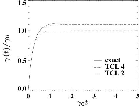
FIG. 1.: Decay rate of the excited state in the damped Jaynes-Cummings model using the time-convolutionless master equation to second (TCL 2) and fourth (TCL 4) order, compared with the exact decay rate. The reservoir correlation time is $\tau_{\rm R}=0.2\gamma_{0}^{-1}$.

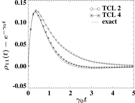
FIG. 2.: Deviation of the population $\rho_{11}(t)$ from the Markovian population $e^{-\gamma_{0}t}$ for the damped Jaynes-Cummings model for the inverse reservoir correlation time $\lambda=5\gamma_{0}$: stochastic simulation (symbols) and exact solution of the time-convolutionless master equation to second (TCL 2) and fourth (TCL 4) order, compared with the exact solution.

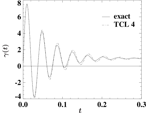
FIG. 3.: Decay rate of the excited state in the damped Jaynes-Cummings model with detuning using the time-convolutionless master equation to fourth order (TCL 4) compared with the exact decay rate. The parameters are: $\gamma_{0}=65$, $\lambda=19.5$, and $\Delta=8\lambda$.

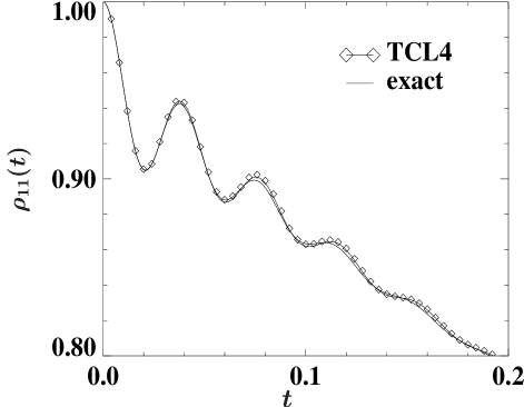
FIG. 4.: Decay of the population $\rho_{11}(t)$ for the damped Jaynes-Cummings model with detuning using the time-convolutionless master equation to fourth order (TCL 4) compared with the exact decay rate. The parameters are: $\gamma_{0}=65$, $\lambda=19.5$, and $\Delta=8\lambda$

REFERENCES

- [1]
- [2] H. Carmichael, An Open Systems Approach to Quantum Optics, Lecture Notes in Physics m18 (Springer-Verlag, Berlin, Heidelberg, New York, 1993).
- [3] J. Dalibard, Y. Castin, and K. Mølmer, Phys. Rev. Lett. 68, 580 (1992).
- [4] N. Gisin and I. C. Percival, J. Phys. A 25, 5677 (1992).
- [5] C. W. Gardiner, A. S. Parkins, and P. Zoller, Phys. Rev. A 46, 4363 (1992).
- [6] H. P. Breuer and F. Petruccione, Phys. Rev. E 52, 428 (1995), Phys. Rev. Lett. 74, 3788 (1995).
- [7] H. M. Wiseman and G. J. Milburn, Phys. Rev. A 47, 1652 (1993).
- [8] H. P. Breuer and F. Petruccione, Fortschr. Phys. 45, 39 (1997).
- [9] H. P. Breuer, W. Huber, and F. Petruccione, Computer Physics Communications 104, 46 (1997).
- [10] S. Chaturvedi and J. Shibata, Z. Physik B 35, 297 (1979).
- [11] N. H. F. Shibata, Y. Takahashi, J. Stat. Phys 17, 171 (1977).
- [12] R. Alicki and K. Lendi, Lecture Notes in Physics: Quantum Dynamical Semigroups and Applications (Springer-Verlag, Berlin, Heidelberg, New York, 1987).
- [13] H. P. Breuer, B. Kappler, and F. Petruccione, Eur. Phys. J. D 1, 9 (1998).
- [14] S. Nakajima, Prog. Theor. Phys 20, 948 (1958).
- [15] R. Zwanzig, J. Chem. Phys 33, 1338 (1960).
- [16] P. Résibois, Physica 27, 721 (1963).
- [17] N. G. van Kampen, Physica 74, 239 (1974).
- [18] B. M. Garraway, Phys. Rev. A 55, 2290 (1996).
- [19] F. Shibata and T. Arimitsu, J. Phys. Soc. Jpn. 49, 891 (1980).