Estimates for practical quantum cryptography

Abstract

In this article I present a protocol for quantum cryptography which is secure against attacks on individual signals. It is based on the Bennett-Brassard protocol of 1984 (BB84). The security proof is complete as far as the use of single photons as signal states is concerned. Emphasis is given to the practicability of the resulting protocol. For each run of the quantum key distribution the security statement gives the probability of a successful key generation and the probability for an eavesdropper’s knowledge, measured as change in Shannon entropy, to be below a specified maximal value.

I Introduction

Quantum Cryptography is a technique for generating and distributing cryptographic keys in which the secrecy of the keys is guaranteed by quantum mechanics. The first such scheme was proposed by Bennett and Brassard in 1984 (BB84 protocol) [1]. Sender and receiver (conventionally called Alice and Bob) use a quantum channel, which is governed by the laws of quantum mechanics, and a classical channel which is postulated to have the property that any classical message sent will be faithfully received. The classical channel will also transmit faithfully a copy of the message to any eavesdropper, Eve. Along the quantum channel a sequence of signals is sent chosen at random from two pairs of orthogonal quantum states. Each such pair spans the same Hilbert space. For example, the signals can be realized as polarized photons: one pair uses horizontal and vertical linear polarization ($+$) while the other uses linear polarization rotated by $45$ degrees ($\times$). Bob at random one of two measurements each performing projection measurements on the basis $+$ or $\times$. The sifted key [2] consists of the subset of signals where the bases of signal and measurement coincide leading to deterministic results. This subset can be found by exchange of classical information without revealing the signals themselves. Any attempt of an eavesdropper to obtain information about the signals leads to a non-zero expected error rate in the sifted key and makes it likely that Alice and Bob can detect the presence of the eavesdropper by comparing a subset of the sifted key over the public channel. If Alice and Bob find no errors they conclude (within the statistical bounds of error detection) that no eavesdropper was active. They then translate the sifted key into a sequence of zeros and ones which can be used, for example, as a one-time pad in secure communication.

Several quantum cryptography experiments have been performed. In the experimental set-up noise is always present leading to a bit error rate of, typically, 1 to 5 percent errors in the sifted key [3, 4, 5, 6]. Alice and Bob can not even in principle distinguish between a noisy quantum channel and the signature of an eavesdropper activity. The protocol of the key distribution has therefore to be amended by two steps. The first is the reconciliation (or error correction) step leading to a key shared by Alice and Bob. The second step deals with the situation that the eavesdropper now has to be assumed to be in the possession of at least some knowledge about the reconciled string. For example, if one collects some parity bits of randomly chosen subsets of the reconciled string as a new key then the Shannon information of an eavesdropper on that new, shorter key can be brought arbitrarily close to zero by control of the number of parity bits contributing towards it. This technique is the generalized privacy amplification procedure by Bennett, Brassard, Crépeau, and Maurer [7].

The final measure of knowledge about the key used in this article is that of change of Shannon entropy. If we assign to each potential key $x$ an a-priori probability $p(x)$ then the Shannon entropy of this distribution is defined as

$$S\left[p(x)\right]=-\sum_{x}p(x)\log p(x)\;.$$ (1)

Note that all logarithms in this article refer to basis $2$. The knowledge Eve obtains on the key may be denoted by $k$ and leads to an a-posteriori probability distribution $p(x|k)$. The difference between the Shannon entropy of the a-priori and the a-posteriori probability distribution is a good measure of Eve’s knowledge:

$$\Delta_{S}(k)=S\left[p(x)\right]-S\left[p(x|k)\right]\;.$$ (2)

For short, we will call $\Delta_{S}(k)$ the entropy change. We recover the Shannon information as the expected value of that difference as

$$I_{S}=\langle\Delta_{S}(k)\rangle=\sum_{k}p(k)\Delta_{S}(k)\;$$ (3)

where Eve’s knowledge $k$ occurs with probability $p(k)$. If we are able to give a bound on $\Delta_{S}(k)$ for a specific run of the quantum key distribution experiment then this is a stronger statement than a bound a the Shannon information: we guarantee not only security on average but make a statement on a specific key, as required for secure communication.

The challenge for the theory of quantum cryptography is to provide a statement like the following one: If one finds $e$ errors in a sifted key of length $n_{\rm sif}$ then, after error correction under an exchange of $N_{\rm rec}$ bits of redundant information, a new key of length $n_{\rm fin}$ can be distilled on which, with probability $1-\alpha$, a potential eavesdropper achieves an entropy change of less than $\Delta_{\rm tol}$. Here $\Delta_{\rm tol}$ has to be chosen in view of the application for which the secret key is used for. It is not necessary that each realization of a sifted key leads to a secret key; the realization may be rejected with some probability $\beta$. In that case Alice and Bob abort the attempt and start anew.

The final goal is to provide the security statement taking into account the real experimental situation. For example, no real channel exist which fulfill the axiom of faithfulness. There is the danger that an eavesdropper can separate Alice and Bob and replace the public channel by two channels: one from Alice to Eve and another one from Eve to Bob. In this separate world scenario Eve could learn to know the full key without causing errors. She could establish different keys with Alice and Bob and then transfer effectively the messages from Alice to Bob. This problem can be overcome by authentication [19]. This technique makes it possible for a receiver of a message to verify that the message was indeed send by the presumed sender. It requires that sender and receiver share some secret knowledge beforehand. It should be noted that it is not necessary to authenticate all individual messages sent along the public channel. It is sufficient to authenticate some essential steps, including the final key, as indicated below. In the presented protocol, successful authentication verifies at the same time that no errors remained after the key reconciliation. The need to share a secret key beforehand to accomplish authentication reduces this scheme from a quantum key distribution system to a quantum key growing system: from a short secret key we grow a longer secret key. On the other hand, since one needs to share a secret key beforehand anyway, one can use part of it to control the flow of side-information to Eve during the stage of key reconciliation in a new way. With side-information we mean any classical information about the reconciled key leaking to the eavesdropper during the reconciliation.

Another problem is that in a real application we can not effectively create single photon states. Recent developments by Law and Kimble [8] promise such sources, but present day experiments use dim coherent states, that is coherent pulses with an expected photon number of typically $1/10$ per signal. The component of the signal containing two or more photon states, however, poses problems. It is known that an eavesdropper can, by the use of a quantum non-demolition measurement of the total photon number and splitting of signals, learn with certainty all signals containing more than one photon without causing any errors in the sifted key. If Eve can get hold of an ideal quantum channel this will lead to the existence of a maximum value of loss in the channel which can be tolerated [9, 10]. It is not known at present whether this QND attack, possibly combined with attacks on the remaining single photons, is the optimal attack but it is certainly pretty strong.

The eavesdropper is restricted in her power to interfere with the quantum signals only by quantum mechanics. In the most general scenario, she can entangle the signals with a probe of arbitrary dimensions, wait until all classical information is transmitted over the public channel, and then make a measurement on the auxiliary system to extract as much information as possible about the key. Many papers, so far, deal only with single photon signals. At present there exists an important claim of a security proof in this scenario by Mayers [11]. However, the protocol proposed there is, up to now, far less efficient than the here proposed one. Other security proofs extend to a fairly wide class of eavesdropping attacks, the coherent attacks [12].

In this paper I will give a solution to a restricted problem. The restriction consists of four points:

• The eavesdropper attacks each signal individually, no coherent or collective attacks take place.

• The signal states consist, indeed, of two pairs of orthogonal single photon states so that two states drawn from different pairs have overlap probability $1/2$.

• Bob uses detectors of identical detection efficiencies.

• The initial key shared by Alice and Bob is secret, that is the eavesdropper has negligible information about it. Using the part of the key grown in a previous quantum key growing session is assumed to be safe in this sense.

Within these assumptions I give a procedure that leads with some a-priori probability $\beta$ to a key shared by Alice and Bob. If successful, the key is secure in the sense that with probability $(1-\alpha)$ any potential eavesdropper achieved an entropy change less than $\Delta_{tol}$. In contrast to all other work on this subject, this procedure takes into account that the eavesdropper does not necessarily transmit single photons to the receiver; she might use multi-photon signals to manipulate Bob’s detectors. The procedure presented here might not be optimal, but it is certifiable safe within the four restrictions mentioned before.

It should be pointed out that coherent eavesdropping attacks are at present beyond our experimental capability. Alice and Bob can increase the difficulty of the task of coherent or collective eavesdropping attacks by using random timing for their signals (although here one has to be weary about the error rate of the key) or by delaying their classical communication thereby forcing Eve to store her auxiliary probe system coherently for longer time. There is an important difference between the threat of growing computer power against classical encryption techniques and the growing power of experimental skills in the attack on quantum key distribution: while it is possible to decode today’s message with tomorrow’s computer in classical cryptography, you can not use tomorrow’s experimental skills in eavesdropping on a photon sent and detected today. It is seems therefore perfectly legal to put some technological restrictions on the eavesdropper. This might be, for example, the restriction to attacks on individual system, or even the restriction to un-delayed measurements. For the use of dim coherent states one might be tempted to disallow Eve to use perfect quantum channels and to give her a minimum amount of damping of her quantum channel. The ultimate goal, however, should be to be able to cope without those restrictions.

The structure of the paper is as follows. In section II I present the complete protocol on which the security analysis is based. Then, in section III I discuss in more detail the various elements contributing to the protocol. The heart of the security analysis is presented in section IV before I summarize in section V the efficiency and security of the protocol.

II How to do quantum key growing

The protocol presented here is a suitable combination of the Bennett-Brassard protocol, reconciliation techniques and authentication methods. I make use of the fact that Alice and Bob have to share some secret key beforehand. Instead of seeing that as a draw-back, I make use of it to simplify the control of the side-information flow during the classical data exchange. Side-information might leak to Eve in the form of parity bits, exchanged between Alice and Bob during reconciliation, or in the form of knowledge that a specific bit was received correctly or incorrectly by Bob. The side-information could be taken care of this during the privacy amplification step using the results of [13]. Here I present for clarity a new method to avoid any such side-information which correlates Eve’s information about different bits (as parity bits do which are typically used in reconciliation) by using secret bits to encode some of the classical communication.

The notation of the variables is guided by the idea that $n_{x}$ denotes numbers of bits, especially key length at various stage, $N_{x}$ denotes numbers of secure bits used in different steps of the protocol, $\beta_{i}$ denote probabilities of failing to establish a shared key, $\alpha_{i}$ denote failure probabilities critical to the safety of an established key, while $\gamma$ denotes the probability that Alice and Bob, unknown to themselves, do not even share a key. Quantities $\overline{x}$ or $\left<x\right>$ denote expected values of the quantity $x$.

The protocol steps and their achievements are:

1. Alice sends a sufficient number of signals to Bob to generate a sifted key of length $n_{\rm sif}$.

2. Bob notifies Alice in which time slot he received a signal.

3. Alice and Bob make a “time stamp” allowing them to make sure that the previous step has been completed before they begin the next step. This can be done, for example, by taking the time of synchronized clocks after step $2$ and to include this time into the authentication procedure.

4. Alice sends the bases used for the signals marked in the second step to Bob.

5. Bob compares this information with his measurements and announces to Alice the elements of the generalized sifted key of length $n_{\rm sif}$. The generalized sifted key is formed by two groups of signals. The first is the sifted key of the BB84 protocol formed by all those signals which Bob can unambiguously interpret as a deterministic measurement result of a single photon signal state. The second group consists of those signals which are ambiguous as they can not be thought of as triggered by single photon signals. If two of Bob detectors (for example monitoring orthogonal modes) are triggered, then this is an example of an ambiguous signal. The number of these ambiguous signals is denoted by $n_{D}$.

   The announcement of this step has to be included into the authentication.

6. Reconciliation: Alice sends, in total, $N_{\rm rec}$ encoded parity-check bits over the classical channel to Bob as a key reconciliation. Bob uses these bits to correct or to discard the errors. During this step he will learn the actual number of errors $n_{\rm err}$. The probability that an error remains in the sifted key is given by $\beta_{1}$. Depending on the reconciliation scheme, Eve learns nothing in this step, or knows the position of the errors, or knows that Bob received all the remaining bits correctly.

7. From the observed number of errors $n_{\rm err}$ and of ambiguous non-vacuum results $n_{D}$ Bob can conclude, using a theorem by Hoeffding, that the expected disturbance measure $\overline{\epsilon}=\left<\frac{n_{\rm err}+w_{D}n_{D}}{n_{\rm sif}}\right>$ is, with probability $1-\alpha_{1}$, below a suitable chosen upper bound $\overline{\epsilon}_{\rm max}$. With probability $1-\beta_{2}$ they find a value for $\alpha_{1}$ which allows them to continue this protocol successfully. Here $w_{D}$ is a weight factor fixed later on.

8. Given the upper bound on the disturbance rate $\overline{\epsilon}_{\rm max}$, Alice and Bob shorten the key by a fraction $\tau$ during privacy amplification such that the Shannon information on that final key is below $I$. The shortening is accomplished using a hash function [19] chosen at random. To make a statement about the entropy change $\Delta_{S}(k)$ Eve achieved for this particular transmission they observe that this change is with probability $1-\alpha_{2}$ less than $\Delta_{\rm tol}$. The probability $\alpha_{2}$ can be estimated by $\alpha_{2}<\frac{I}{\Delta_{\rm tol}}$.

9. In the last step Alice chooses at random a suitable hash function which she transmits encrypted to Bob using $N_{\rm aut}/2$ secret bits. Then she hashes with that function her new key, the time from step $3$, and the string of bases from step $5$ into a short sequence, called the authentication tag, The tag is sent to Bob who compares it with the hashed version of his key. If no error was left after the error correction the tags coincide.This step is repeated with the roles of Alice and Bob interchanged. If Bob detects an error rate too high to allow to proceed with the protocol, he does not forward the correct authentication to Alice. The probability Eve could have guessed the secret bits used by Alice or by Bob to encode their hashed message is given by $\alpha_{3}$. The probability that a discrepancy between the two versions of the key remains undetected is denoted by $\gamma$.

The probability of detected failure is $\beta$ with $\beta<\beta_{1}+\beta_{2}$ and this failure does not compromise the security. In the case of success Alice and Bob can now say that, at worst, with a probability of undetected failure (failure of security) of $\alpha$ (with $\alpha<\alpha_{1}+\alpha_{2}+\alpha_{3}$) the eavesdropper can achieve an entropy change for the final key which is bigger than $\Delta_{\rm tol}$. The remaining probability $\gamma$ describes the probability that Alice and Bob do not detect that they do not even share a key.

Note that the final authentication is made symmetric so that no exchange of information over the success of that step is necessary. Otherwise a party not comparing the authentication tags could regard the key as safe in a separate-world scenario. More explanation about the authentication procedure can be found in section III E. The classical information becoming available to Eve during the creation of the sifted key will be taken care of in the calculations of section IV.

The public channel is now used for the following tasks:

• creation of the sifted key, where Eve learns which signals reached Bob and from which signal set each signal was chosen from,

• transmission of encrypted parity check bits, on which Eve learns nothing,

• for bi-directional reconciliation methods: feedback concerning the success of parity bit comparisons (see following section),

• for reconciliation methods which discard errors: the location of bits discarded from the key,

• announcement of the hash function chosen in this particular realization,

• transmission of the encrypted hash function for authentication and of the unencrypted authentication tags.

The main subject of this paper is to give the fraction $\tau$ by which the key has to be shortened to match the security target as a function of the upper bound on the disturbance $\overline{\epsilon}_{\rm max}$. The estimation has to take care of all information available to Eve by a combination of measurements on the quantum channel and classical information overheard on the public channel. This classical information depends on the reconciliation procedure used. The nature of this information might allow Eve to separate the signals into subsets of signals, for example those being formed by the signals which are correctly (incorrectly) received by Bob, and to treat them differently.

The knowledge of the specific hash function is of no use to Eve in construction of her measurement on the signals. This is a result of the assumption that Eve attacks each signal individually and that the knowledge of the hash functions tells Eve only whether a specific bit will count towards the parity bit of a signal subset or not. She only will learn how important each individual bit is to her. If the bit is not used then it is too late to change the interaction with that bit to avoid unnecessary errors, since the damage by interaction has been done long before. If it is used, then Eve intends to get the best possible knowledge about it anyway. This situation might be different for scenarios which allow coherent attacks.

III Elements of the quantum key growing protocol

In this section I explain in more detail the steps of the quantum key growing protocol. Special attention is given to the security failure probabilities $\alpha_{i}$, limiting the security confidence of an established shared key, and to the failure probabilities $\beta_{i}$, limiting the capability to establish a shared key.

A Generation of the generalized sifted key

Elements of the generalized sifted key are signals which either can be unambiguously interpreted as being deterministicly detected, given the knowledge of the polarization basis, or which trigger more than one detector. We think of detection set-ups where detectors monitor one relevant mode each. Due to loss it is possible to find no photon in any mode. Since Eve might use multi-photon signals we may find photons in different monitored modes simultaneously, leading to ambiguous signals since more than one detector gives a click. Detection of several photons in one mode, however, is deemed to be an unambiguous result. (See further discussion in section IV B.) In practice we will not be able to distinguish between one or several photons triggering the detector. The length of the sifted key accumulated in that way is kept fix to be of length $n_{\rm sif}$.

B Reconciliation

For the reconciliation we have to distinguish two main classes of procedures: one class corrects the errors using redundant information and the other class discards errors by locating error-free subsections of the sifted key. The class of error-correcting reconciliation can be divided in two further subclasses: one subclass uses only uni-directional information flow from Alice to Bob while the second subclass uses an interactive protocol with bi-directional information flow.

The difference between the three approaches with respect to our protocol shows up in the number of secret bits they need to reconcile the string, the length of the reconciled string, and the probability of success of reconciliation. For experimental realization one should think as well of the practical implementation. For example, interactive protocols are very efficient to implement [14]. To illustrate the difference I give examples for the error correction protocols.

The benchmark for efficiency of error correction is the Shannon limit. It gives the minimum number of bits which have to be revealed about the correct version of a key to reconcile a version which is subjected to an error rate $e$. This limit is achieved for large keys and the error correction probability approaches then unity. The Shannon limit is given in terms of the amount of Shannon information $I_{S}(e)$ contained in the version of the key affected by the error rate $e$. For a binary channel, as relevant in our case, this is given by

$$I_{S}(e)=1+e\log e+(1-e)\log(1-e)\;.$$ (4)

The minimum number of bits needed, on average, to correct a key of length $n$ affected by the error rate $e$ is then given by

$$n_{\rm min}=n\;\left\{1-I_{S}(e)\right\}\;.$$ (5)

As mentioned before, perfect error correction is achievable only for $n\to\infty$.

1 Linear Codes for error correction.

Linear codes are a well-established technique which can be viewed in a standard-approach as attaching to each $k$-bit signal a number of $(n-k)$ bits of linearly independent parity-check bits making it in total a $n$-bit signal. The receiver gets a noisy version of this n-bit signal and can now in a well-defined procedure find the most-likely $k$-bit signal. Linear codes which will safely return the correct $k$-bit signal if up to $f$ of the $n$ bits were flipped by the noisy channel are denoted by $[n,k,d]$ codes (with $d=2f+1$). If the signal is affected by more errors then these will be corrected with less than unit probability.

This technique can be used for error correction. Alice and Bob partition their sifted key into blocks of size $k$. For each block Alice computes the extra $n-k$ parity bits, encodes them with secret bits and sends them via the classical channel to Bob. Bob then corrects his block according to the standard error correction technique. This procedure could be improved, since the $[n,k,d]$ codes are designed to cope with the situation that even the parity bits might be affected by noise. One can partly take advantage of the situation that these bits are transmitted correctly. However, non-optimal performance is not a security hazard.

The search for an optimal linear code is beyond the scope of this paper. To illustrate the problem I present as specific example the code $[512,422,21]$. It uses $90$ redundant parity bits to protect a block of $422$ bits against $10$ errors. So how does this linear code perform if we use it to reconcile a string of $n_{\rm sif}=10128$ bits which are affected by an error rate of $1\%$? It can be shown that this string will be reconciled with a probability of $(1-\beta_{1})=0.908$ at an expense of $N_{\rm rec}=2160$ secret bits. The practical implementation of a code as long as this one is, however, rather problematic from the point of view of computational resources. In comparison, in the Shannon limit we need to use $819$ bits for this task.

2 Interactive error correction

An interactive error correction code was presented by Brassard and Salvail in [14]. This code is reported to correct a key with an error rate of $1\%$ and length $n_{\rm sif}=10000$ at an average expense of $N_{\rm rec}=933$ bits. No numbers for $\beta_{1}$ are given, but in several tries no remaining error was found. This protocol operates acceptable close to the Shannon limit which tells us that we need at least $808$ bits to correct the key.

3 Situation after reconciliation

After reconciliation Alice and Bob share with probability $(1-\beta_{1})$ the same key. The eavesdropper gathered some information from measurements on the quantum channel. The information she gained from listening to the public channel puts her now into different positions depending on the reconciliation protocol. In case errors are discarded, she knows that all remaining bits in the reconciled string were received correctly by Bob during the quantum transmission. If an uni-directional error correction protocol is used, then listening to the public channel during reconciliation does not give Eve any extra hints. The interactive error correction protocol, however, leaks some information to Eve about the position of bits which were received incorrectly by Bob during the quantum protocol. We will have to take this into account later on. There we take the view that Eve knows the positions of all errors exactly.

A difference between correcting and discarding errors is that, naturally, discarding errors will lead to a shorter reconciled string of length $n_{\rm rec}<n_{\rm sif}$, while the length of the key does not change during error correction so that $n_{\rm rec}=n_{\rm sif}$. Common to all schemes is that Alice and Bob know the precise number of errors which occurred (provided the reconciliation worked). When they discard parts of the sifted key they can open up the discarded bits and learn thereby the actual number of errors (although in this case an additional problem of authentication arises), and when they correct errors Bob knows the number of bit-flips he performed during error correction. This is just the number of errors of the sifted key.

Contrary to common belief it is therefore not necessary to sacrifice elements of the sifted key by public comparison to determine or estimate the number of occurred errors.

C Privacy amplification and the Shannon information on final key

In previous work it has been shown that for typical error rates in an experimental set-up the eavesdropper could gain, on average, non-negligible amount of Shannon information on the reconciled key [15, 16]. This means that we can not use it as a secret key right away. Classical coding theory shows a way to distill a final secret key from the reconciled key by the method of privacy amplification [7]. As a practical implementation of the hashing involved, the secret key is obtained by taking $n_{\rm fin}$ parity bits of randomly chosen subsets of the $n_{\rm rec}$ bits of the reconciled string. The choice of the random subsets is made only at that instance and changes for each repetition of the key growing protocol. This shortening of the key to enhance the security of the final key is common to all other approaches that deal with the security of quantum cryptography, for example by Mayers [11] or Biham et al [12]. However, it differs the way to determine the fraction $\tau$ by which the key has to be shortened. In the case of individual eavesdropping attacks we can go via the collision probability as described below [7]. When we consider joint or collective attacks it is not possible to take this approach due to correlation between the signals which possibly allows Eve to gain an advantage by delaying her measurement until she learns to know the specific parity bits entering the final key.

In the first step we give the main formulas of privacy amplification and introduce the parameter $\tau_{1}(\overline{\epsilon})$. This parameter indicates the fraction by which the key has to be shortened such that the expected eavesdropping information on the final key is less than 1 bit of Shannon information. It is given as a function of Eve’s acquired collision probability. Any additional bit by which the key is shortened leads to an exponential decrease of that expected Shannon information.

We denote by $z$ the final key of length $n_{\rm fin}$, by $x$ the reconciled key of length $n_{\rm rec}$ and by $y$ the accumulated knowledge of the eavesdropper due to her interaction with the signals and the overheard classical communication via the public channel. We keep separately the hash function $g$ which, for example, describes the subsets whose parity bits form the final key. This hash function is part of Eve’s knowledge in each realization. Eve’s knowledge is expressed in a probability distribution $p(z|g,y)$, that is the probability that $z$ is the key given Eve’s measurement results and side-information on the key. In a trivial extension of the starting equation of [7] we find that the Shannon information $\tilde{I}$, averaged over the hash functions, is bounded by

$$I\equiv\langle\tilde{I}\rangle_{g}\leq n_{\rm fin}+\log\langle p_{c}^{z}(g,y)\rangle_{y,g}$$ (6)

with the collision probability on the final key defined as $p_{c}^{z}(g,y)=\sum_{z}p^{2}(z|g,y)$. The collision probability $\langle p_{c}^{z}(g,y)\rangle_{g}$ on the final key, averaged with respect to $g$, is bounded by the collision probability $p_{c}^{x}(y)=\sum_{x}p^{2}(x|y)$ on the reconciled key as

$$\langle p_{c}^{z}(g,y)\rangle_{g}<2^{-n_{\rm fin}}\left(2^{n_{\rm fin}}p_{c}^{x}(y)+1\right)\;.$$ (7)

This can be trivially extended to an inequality for $\langle p_{c}^{z}(g,y)\rangle_{y,g}$ resulting in

$$\langle p_{c}(g,y)\rangle_{g,y}<2^{-n_{\rm fin}}\left(2^{n_{\rm fin}}\langle p_{c}^{x}(y)\rangle_{y}+1\right)\;.$$ (8)

This allows us to give the estimate

$$I\leq\log\left(2^{n_{\rm fin}}\langle p_{c}^{x}(y)\rangle_{y}+1\right)\;$$ (9)

bounding the eavesdropper’s expected Shannon information by her expected collision probability on the sifted key and the length of the final key.

We can reformulate the estimate (9) by introducing the fraction $\tau_{1}$. If we shorten the reconciled key by this fraction then Eve’s expected Shannon information is just one bit on the whole final key. Therefore we find

$$\tau_{1}=1+\frac{1}{n_{\rm rec}}\log\langle p_{c}^{x}(y)\rangle_{y}\;.$$ (10)

We introduce the security parameter $n_{S}$ as the number of bits by which the final key is shorter than prescribed by the fraction $\tau_{1}$. This security parameter $n_{S}$ is implicitly defined by

$$n_{\rm fin}=(1-\tau_{1})\;n_{\rm rec}-n_{S}\;.$$ (11)

With the definitions of $\tau_{1}$ and $n_{S}$ we then find [7]

$$I\leq\log(2^{-n_{S}}+1)\approx\frac{2^{-n_{S}}}{\ln 2}\;.$$ (12)

From this relation we see that the total amount of Eve’s expected Shannon information on the final key decreases exponentially with the security parameter $n_{S}$. The main part of this paper will be to estimate $\langle p_{c}^{x}(y)\rangle_{y}$ for various scenarios as a function of the expected disturbance rate $\overline{\epsilon}$ to estimate $\tau_{1}$ and with that to estimate $I$ as a function $\overline{\epsilon}$.

D From expected quantities to specific quantities

In the previous section we showed that once we know the expected disturbance rate $\overline{\epsilon}$ and the functional dependence of $\tau_{1}(\overline{\epsilon})$, we can estimate the eavesdropper’s Shannon information $I$ on the final key in dependence of $n_{S}$ via equation (12). In this section we now show how to link the observed error rate to the expected error rate and how to estimate the entropy change $\Delta_{S}$ in a single run from the expected Shannon information $I$.

1 From the measured error rate to the expected error rate

Alice and Bob establish a generalized sifted key of length $n_{\rm sif}$. During reconciliation of the sifted key Bob learns the actual number of errors $n_{\rm err}$ of unambiguous signals while he already knows the number $n_{D}$ of ambiguous signals. Our definition of disturbance is here

$$\epsilon=\frac{n_{\rm err}+w_{D}n_{D}}{n_{\rm rec}}$$ (13)

with $w_{D}$ as adjustable weight parameter for ambiguous signals to be chosen in a suitable way. We will present in section IV G a model for which we can choose $w_{D}=1/2$. In the case of error correction we have to correct even the ambiguous signals to keep the number $n_{\rm sif}$ fixed and to keep control about the disturbance. The reason is we need to formulate a measure of disturbance per element of the reconciliated key which is bounded. This is possible for correction of errors. In the case of discarding errors the number of errors and ambiguous results per remaining bit is unbounded and we fail to be able to give a bound on $\overline{\epsilon}$ from the measured values.

Therefore we restrict ourselves to the case of corrected errors where we find the length $n_{\rm rec}$ of the reconciled string to be equal to the length $n_{\rm sif}$ of the generalized sifted key. In this situation the measured disturbance is given by $\epsilon_{\rm meas}=\frac{n_{\rm err}+w_{D}n_{D}}{n_{\rm sif}}$. Since $n_{\rm sif}$ is kept fixed the expected disturbance is given by $\overline{\epsilon}=\frac{\left<n_{\rm err}+w_{D}n_{D}\right>}{n_{\rm sif}}$. From the measured value $\epsilon_{\rm meas}$ we estimate the average disturbance parameter $\overline{\epsilon}$.

To make the role of $\overline{\epsilon}$ clear it should be pointed out that any given eavesdropping strategy will lead to an expected error probability $\overline{\epsilon}$ while the actually caused and observed error rate can be much lower for an individual run of the protocol. For example, think of an intercept/resend protocol as in [10] where Eve has her lucky day and measures, by chance, all signals in the appropriate bases. This is not very likely, but the treatment presented here takes care of this possibility.

In an application of a theorem by Hoeffding [17], which has been used already in [12], we find an estimate of the number $\left<n_{\rm err}+w_{D}n_{D}\right>$ from the actually measured number $n_{\rm err}+w_{D}n_{D}$ for a total number of $n_{\rm sif}$ signals as

$$\left<n_{\rm err}+w_{D}n_{D}\right><n_{\rm err}+w_{D}n_{D}+n_{\rm sif}\delta$$ (14)

with probability

$$(1-\alpha_{1})>1-\exp(-2n_{\rm sif}\delta^{2})$$ (15)

as long as $w_{D}\leq 1$. For $w_{D}\geq 1$ we have to replace equation (15) by $(1-\alpha_{1})>1-\exp(-\frac{2n_{\rm sif}\delta^{2}}{w_{D}^{2}})$. This means that we can give a bound on the expected disturbance parameter $\overline{\epsilon}$ from the observed quantities $n_{D}$ and $n_{\rm err}$ within a certain confidence limit. To give a numeric example we choose $w_{D}=1/2$ (see section IV G) and refer to the situation reported by Marand and Townsend [3]. There an experiment is presented which can create a sifted key of length $n_{\rm sif}=1.4\times 10^{-3}n$ from an exchange of $n$ quantum signals at an error rate of $1.2\%$ with a negligible amount of ambiguous signals. Then the choice of $\delta=0.038$ and a sampling with $n=10^{7}$ leads to a reconciled key of length $n_{\rm sif}=1.4\times 10^{4}$ with a value of $\alpha_{1}\approx 10^{-18}$. This is the probability that the expected disturbance parameter $\overline{\epsilon}$ in a typical realization of the key transfer is less than a maximal value of $\overline{\epsilon}_{\rm max}=0.05$. The value $\overline{\epsilon}_{\rm max}$ will be used in privacy amplification. An eye has to be kept on the sampling time. With the experiment described in [3] it will take about $10$ seconds to establish the sifted key. An example for smaller samples is the choice of $n=10^{5}$ and $\delta=0.4$ which leads for the same system to a reconciled key of length $n_{\rm sif}=140$ and $\alpha_{1}\approx 10^{-19}$, $\overline{\epsilon}_{\rm max}=0.412$. The probability $\beta_{2}$ to fail to achieve a satisfactory level of confidence at this stage is in most cases negligible in comparison to the failure of reconciliation. It should be noted that these numbers give a rough guidance only, since the experiment does not use single-photon signals.

2 Expected information and information in specific realization

We still need to link the change of Shannon entropy $\Delta_{S}$ on the final key in an individual realization of the protocol with a given probability to the Shannon information $I$, that is over the average over many realizations. The key is thought of as unsafe if the eavesdropper achieves an entropy change bigger than $\Delta_{\rm tol}$ in a specific realization. This happens at most with probability $\alpha_{2}$ which is bounded implicitly by $I>\alpha_{2}\Delta_{\rm tol}$ leading to

$$\alpha_{2}<\frac{I}{\Delta_{\rm tol}}=\frac{\log(2^{-n_{S}}+1)}{\Delta_{\rm tol}}\approx\frac{2^{-n_{S}}}{\Delta_{\rm tol}\ln 2}$$ (16)

So the knowledge of an estimate for $I$ and the prescription of an acceptable value of $\Delta_{\rm tol}$ gives us the probability $1-\alpha_{2}$ of secrecy of the key.

E Authentication

The tools of the previous sections allow Alice and Bob to construct a common secret key provided that their classical channel is faithful. Since channels with that property, as such, do not exist, we need to authenticate the procedure to make sure that Alice and Bob actually share the new key. Authentication can protect at the same time against errors which survived the reconciliation step and against an eavesdropping attack with a “separate world” approach.

It is essential to make sure that Eve has no influence on the choice of bits entering the generalized sifted key exceeding the power to manipulate the quantum channel. The time-stamp step $3$ in the protocol assures us that there is no point in Eve faking the public discussion up to that point since she gained no additional information about the signals so far, especially no information about the polarization basis.

The following sequence of bases for the successful received signals sent from Alice and Bob does not need to be authenticated as well since Eve can not bar corresponding signals from the sifted key without knowing Bob’s measurements as well. However, the message describing which bits finally form the generalized sifted key needs to be authenticated since Eve is now in the position to bar signals from the sifted key she shares with Alice by manipulation of the contents of the message [18].

The subsequent reconciliation protocol need not to be authenticated if we authenticate the final key. The reason for that is that the previous steps fixed the reconciled key as the generalized sifted key in Alice’s version. If Eve tampers with the reconciliation protocol then Bob will fail correct his key so that it becomes equal to Alice’s key. Authentication of the final key will therefore be sufficient to protect against tampering with the public channel in this step. It doubles at the same time to protect against incomplete reconciliation.

To summarize, we need to authenticate the string identifying the elements of the sifted key within the received signals, the time stamp, and the final key. The length of this string is roughly $m\approx 2n_{\rm sif}$. The authentication is done in the following way which is based on the authentication procedure of Wegman and Carter [19]:

Alice chooses a hash-function of approximate length $N_{\rm aut}/2=4t\log m$ and sends it encrypted to Bob. Both evaluate the hashed version of the message, the tag, of length $t$. Alice sends the tag via the public channel to Bob. If the tags coincide then this step is repeated with the role of Alice and Bob interchanged. With this symmetric scheme we make sure that neither Alice nor Bob can be coaxed into a position where they think that authentication succeeded when it in fact failed. The probability that Eve could fake the authentication is given by

$$\alpha_{3}=2^{-t+1}\;.$$ (17)

This is at the same time the probability that two distinct final keys lead to the same hashed key. Any remaining error in the final key will therefore lead with probability $1-\alpha_{3}$ to a failure of the authentication.

IV Expected collision probability and expected error rate

This section represents the major input of physics to the quantum key growing protocol. The aim is to put an upper bound on the expected average collision probability Eve obtains on the reconciliated key as a function of an average disturbance rate her eavesdropping strategy inflicted on the signals. This is done for two methods of reconciliation, correcting or deleting errors. The result will allow us to give values for the parameter $\tau_{1}(\overline{\epsilon})$.

A Collision probability on individual signal

The collision probability on the reconciled key is defined by

$$p_{c}^{x}(y)=\sum_{x}p^{2}(x|y)\;.$$ (18)

We assume that the signal sent by Alice are statistically independent of each other and Eve interacts with and performs measurements on each bit individually. Furthermore, we avoid side-information which correlates signals by the use of secret bits in the reconciliation step. Therefore the conditional probability function $p(x|y)$ for $x$ being the key given Eve’s knowledge $y$ factorises into a product of probabilities for each signal. With that the expected collision probability factorises as well into a product of the expected collision probability for each bit. We denote by $p_{c}^{x}$ the expected collision probability on one bit so that

$\displaystyle\langle p_{c}^{x}(g,y)\rangle_{y}=\left(p_{c}^{x}\right)^{n_{\rm rec}}$

Furthermore, we denote by the index $\alpha\in\{+,\times\}$ the two conjugate bases (e.g. horizontal or vertical polarization for single photons) used to encode the signals, by $\Psi\in\{0,1\}$ the logical values, and by $k$ the possible outcomes of Eve’s measurement. This leads to an expression of the expected collision probability, at this stage, as

$$p_{c}^{x}=\sum_{k,\Psi,\alpha}\frac{p^{2}(\Psi_{\alpha},k_{\alpha})}{p(k_{\alpha})}\;.$$ (19)

We find for the parameter $\tau_{1}$ describing the shortening of the key during privacy amplification from eqn. (10)

$$\tau_{1}=\log(2p_{c}^{x})\;.$$ (20)

B Eve’s interaction and detection description

The action of the eavesdropper can be described by a completely positive map [20, 21] acting on the signal density matrices $\rho$ as

$$\tilde{\rho}=\sum_{k}A_{k}\rho A_{k}^{\dagger}$$ (21)

where we can associate this interaction with a measurement by Eve of a Probability Operator Measure (POM) formed by the operators $F_{k}=A_{k}^{\dagger}A_{k}$. The operators $A_{k}$ are arbitrary operators mapping the Hilbert space of the signals to an arbitrary Hilbert space. The only restriction is that $\sum_{k}A_{k}^{\dagger}A_{k}$ gives the identity operator of the signal Hilbert space. The probability for occurrence of outcome $k$ is then given by $p(k)={\rm Tr}(\rho F_{k})$. The action of Bob’s detectors can be described by a POM on the resulting Hilbert space after Eve’s interaction. Since the detection POM elements and the signal density operators can be represented by real matrices, we can assume the operators $A_{k}$ to be represented by real matrices as well.

This does not limit the generality of the approach, since the outcome corresponding to an operator $A_{k}=A_{k}^{\rm re}+iA_{k}^{\rm im}$, with real operators $A_{k}^{\rm re}$ and $A_{k}^{\rm im}$, is triggered with probability ${\rm Tr}(\rho{A_{k}^{\rm re}}^{\dagger}A_{k}^{\rm re})+{\rm Tr}(\rho{A_{k}^{\rm im}}^{\dagger}A_{k}^{\rm im})$ and the outcome probabilities for Bob’s detection, corresponding to POM element $F$ if outcome $k$ of Eve’s measurement is being triggered, is given by ${\rm Tr}(A_{k}^{\rm re}\rho{A_{k}^{\rm re}}^{\dagger}F)+{\rm Tr}(A_{k}^{\rm re}\rho{A_{k}^{\rm re}}^{\dagger}F)$. Since no cross-terms mixing $A_{k}^{\rm re}$ and $A_{k}^{\rm im}$ occur this means that using the two real operators $A_{k}^{\rm re}$ and $A_{k}^{\rm im}$, instead of $A_{k}=A_{k}^{\rm re}+iA_{k}^{\rm im}$, will not change the outcome probabilities of Bob’s detectors but refines Eve’s measurement.

Two typical detection set-ups are shown in figure 1. The active version consists of a polarization analyzer (two detectors monitoring each an output of a polarizing beam-splitter) and a phase shifter which effectively changes the polarization basis of the subsequent measurement. Here one has actively to choose the polarization basis of the measurement. The passive device uses two polarization analyzers, one for each basis, and uses a beam-splitter to split the incoming signal the two polarization analyzers are used with equal probability for detection.

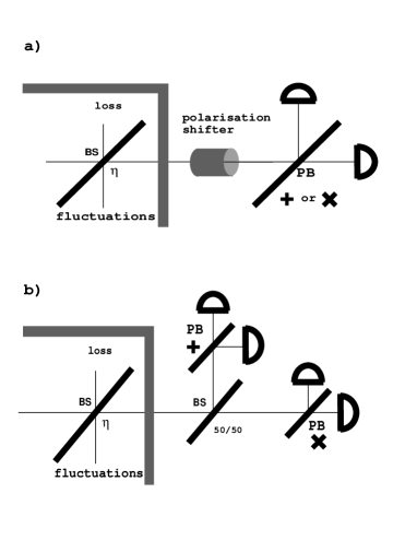
FIG. 1.: (a) Active device: Bob’s two detectors consist each of a polarizing beam splitter and an ideal detector. The polarizing beam splitter discriminates the two orthogonal linear polarized modes. Using a polarization shifter the polarization basis can be changed as desired. Detector efficiencies are modeled by a beam splitter which represents the loss and which is thought of as being part of the eavesdropper’s strategy. This beam splitter can be seen as part of the quantum channel. (b) Passive device: Here one uses two detection modules as presented in (a), one for each polarization basis. The central beam-splitter takes the task to “switch” between the two polarization analyzers.

One can represent the detectors by beam-splitters combined with ideal detectors [22]. Then the beam-splitters can be thought to be responsible for the finite efficiency. Since all detectors are assumed to be equal, the losses of all detectors involved can be attributed to a single loss beam-splitter, which is then thought of as being part of the transmission channel rather than being part of the detection unit.

We can use the idea of ideal detectors which measure each a POM with two elements, the projection operator onto the vacuum (no “click”) and the projection on the Fock-subspaces with at least one photon (“click”). The POM of the active and the passive set-up then contains the elements $F_{\rm vac}$, $F_{0_{+}}$, $F_{1_{+}}$, $F_{0_{\times}}$, $F_{1_{\times}}$, $F_{D}$. These are projections onto the vacuum, $F_{\rm vac}$, onto states with at least one photon in one of the four signal polarizations and none in the others, therefore leading to an unambiguous result, $F_{\Psi_{\alpha}}$, and onto the rest of the Hilbert space, that is onto all states containing at least one photon in the signal polarization and at least one in an orthogonal mode $F_{D}$. The first POM outcome manifests itself in no detector click at all, the following four give precisely one detector click, and the last one gives rise to at least two detectors being triggered. If we denote by $|n,m\rangle_{\alpha}$ the state which has $n$ photons in one mode and $m$ photons in the orthogonal polarization mode with respect to the polarization basis $\alpha$, use the abbreviation $E^{(0)}$ for the projector onto the vacuum and $E^{(n)}_{\Psi_{\alpha}}$ for the projector onto the state with $n$ photons in the polarization mode corresponding to $\Psi_{\alpha}$, then the POM of detection unit (a) is given by

$$F_{\rm vac} = E^{(0)}$$ (22)

$$F_{\Psi_{\alpha}} = \frac{1}{2}\sum_{n=1}^{\infty}E^{(n)}_{\Psi_{\alpha}}$$ (23)

$$F_{D} = \frac{1}{2}\sum_{n,m=1}^{\infty}|n,m\rangle_{+}\langle n,m|+\frac{1}{2}\sum_{n,m=1}^{\infty}|n,m\rangle_{\times}\langle n,m|\;.$$ (24)

On the other hand, the passive detection scheme (b) is more susceptible to signals containing more than one photon. It is described by the POM

$$F_{\rm vac} = E^{(0)}$$ (25)

$$F_{\Psi_{\alpha}} = \sum_{n=1}^{\infty}\left(\frac{1}{2}\right)^{n}E^{(n)}_{\Psi_{\alpha}}$$ (26)

$$F_{D} = \sum_{n=1}^{\infty}\left[\left(\frac{1}{2}-\left(\frac{1}{2}\right)^{n}\right)\sum_{\Psi,\alpha}E^{(n)}_{\Psi,\alpha}\right]$$ (28)

$$+\frac{1}{2}\sum_{n,m=1}^{\infty}|n,m\rangle_{+}\langle n,m|+\frac{1}{2}\sum_{n,m=1}^{\infty}|n,m\rangle_{\times}\langle n,m|\;.$$

The next idea concerns all detection set-ups where all elements of the POM commute with the projections $E_{n}$ onto the subspaces of total photon number $n$. In that case we find that Bob’s measurement on the final signal gives outcome $i\in\{{\rm vac},\Psi_{\alpha},D\}$ with probability

$$P_{\rm Bob}(i):={\rm Tr}(\sum_{k}A_{k}\rho A_{k}^{\dagger}F_{i})={\rm Tr}(\sum_{k,n}E_{n}A_{k}\rho A_{k}^{\dagger}E_{n}F_{i})$$

We can now replace the set of $A_{k}$’s by the set $A_{n,k}:=E_{n}A_{k}$ which still describes Eve measurement but for which each element maps the Hilbert space of the signals to a Hilbert space with a fixed photon number. Eve will now associate a POM element of her measurement with each such $A_{n,k}$ thereby refining her POM and leading to an increase of her knowledge. For short we write again $A_{k}$ for this set, for which now the property is assumed that the signal arriving at Bob’s detection unit is an eigenstate of the total photon number operator. We can divide the index set $K$ of $k$ into subsets $K^{(n)}$ so that for each $k\in K^{(n)}$ the operator $A_{k}$ maps the one-photon Hilbert space of the signal into the $n$-photon space. This is useful to distinguish contributions of signals with different photon number.

We still have to discuss how to represent a delayed measurement in this picture. A delayed measurement is performed in the way that Eve brings an auxiliary system into contact with the signal so that they evolve together under a controlled unitary evolution. Then the signal is measured by Bob while Eve delays the measurement of her auxiliary system until she has received all classical information exchanged over the public channel. Having this knowledge, she picks the optimal measurement to be performed on her auxiliary system. Classical information useful to Eve is information that allows her to divide the signals into subsets which should experience different treatment. In our situation this information is represented by the polarization basis of the signal and, for bi-directional error correction, by the knowledge whether the signal was received correctly by Bob. We have therefore to assume, for example, that Eve’s delayed measurement is characterized by the set of operators $A_{k}$ with $k\in K$, giving rise to Eve’s POM $F_{k}=A_{k}A_{k}^{\dagger}$, and which are applied to the signals from the set $\alpha=\mbox{``$+$''}$ and a second set $B_{k^{\prime}}$ with $k^{\prime}\in K^{\prime}$, resulting in the POM $F^{\prime}_{k^{\prime}}=B_{k^{\prime}}B_{k^{\prime}}^{\dagger}$, which are applied to the signals from the set $\alpha=\mbox{``$\times$''}$. Of course, these two sets of operators can not be chosen arbitrarily. The complete positive map has to be identical for all density matrices $\rho$, that is

$$\tilde{\rho}=\sum_{k\in K}A_{k}\rho A_{k}^{\dagger}=\sum_{k^{\prime}\in K^{\prime}}B_{k^{\prime}}\rho B_{k^{\prime}}^{\dagger}\;.$$ (29)

Moreover, this equality holds even for non-Hermitian matrices $\rho$. We can combine this result with the partition into $n$-photon subspaces. Then we find that even the stronger statement

$$\sum_{k\in K^{(n)}}A_{k}\rho A_{k}^{\dagger}=\sum_{k^{\prime}\in K^{\prime(n)}}B_{k^{\prime}}\rho B_{k^{\prime}}^{\dagger}\;.$$ (30)

holds. Before we go on to the derivation of the relation between average disturbance and average collision probability I would like to point out that this treatment takes into account the rich structure of modes supported by optical fibers and the fact that detectors monitor a multitude of modes. As long as the detection POM commutes with the projector onto the actually used signal mode, which is usually the case, we can separate the action of the $A_{k}$ with respect to the photon number in a similar way.

C Separation into $n$-photon contributions

In this section we are going to present the disturbance measure $\epsilon$ and the collision probability $\ p_{c}^{x}$ as sums over contributions with different definite photon number $n$ arriving at Bob’s detector unit. We start from the definition of the disturbance $\epsilon$. To allow some comparison between correcting and discarding errors, we present a unified definition which defines, even for discarded errors, a disturbance measure per bit of the reconciled key. This definition is given by

$$\epsilon=\frac{n_{\rm err}+w_{D}n_{D}}{n_{\rm rec}}\;.$$ (31)

Here $n_{\rm err}$ is the number of errors in the sifted key, $n_{D}$ is the number of ambiguous results occurring and $n_{\rm rec}$ is the number of bits in the reconciled string. The weight parameter $w_{D}$ for ambiguous signals will be fixed later on. If we keep the size of the reconciled key fixed, then the expectation value of $\epsilon$ is described by

$$\overline{\epsilon}=\frac{p_{\rm err}+w_{D}p_{D}}{p_{\rm rec}}\;$$ (32)

where $p_{\rm err},p_{D},p_{\rm rec}$ are the absolute probabilities that a signal will, respectively, enter the sifted key as error, cause an ambiguous result, or become an element of the reconciled key. As mentioned before, it should be noted, that no estimate $\overline{\epsilon}$ from measured data can be easily presented in the case of discarded errors. We separate the contributions from the different photon number signals as

$$\overline{\epsilon}=\sum_{n}\frac{p_{\rm rec}^{(n)}}{p_{\rm rec}}\frac{p_{\rm err}^{(n)}+w_{D}p_{D}^{(n)}}{p_{\rm rec}^{(n)}}=\sum_{n}\frac{p_{\rm rec}^{(n)}}{p_{\rm rec}}\overline{\epsilon}^{(n)}\;.$$ (33)

where we have implicitly defined

$$\overline{\epsilon}^{(n)}=\frac{p_{\rm err}^{(n)}+w_{D}p_{D}^{(n)}}{p_{\rm rec}^{(n)}}$$ (34)

as the n-photon contribution towards the disturbance measure. Now $p_{X}^{(n)}$ are the conditional probabilities that a signal has property $X$ while being transfered as $n$-photon signal between Eve and Bob. The total disturbance is given as sum over the n-photon contribution weighted by the relative probability that a signal arriving as an n-photon signal at Bob’s detector will enter the reconciled key.

If we discard errors, then we find for the relevant probabilities (with $\overline{\Psi}$ as the complement to binary value $\Psi$)

$$p_{\rm err}^{(n)} = \frac{1}{4}\sum_{k\in K^{(n)}\atop\Psi,\alpha,}{\rm Tr}\left(A_{k}\rho_{\Psi_{\alpha}}A_{k}^{\dagger}F_{\overline{\Psi}_{\alpha}}^{(n)}\right)$$ (35)

$$p_{\rm rec}^{(n)} = \frac{1}{4}\sum_{k\in K^{(n)}\atop\Psi,\alpha,}{\rm Tr}\left(A_{k}\rho_{\Psi_{\alpha}}A_{k}^{\dagger}F_{\Psi_{\alpha}}^{(n)}\right)$$ (36)

$$p_{D}^{(n)} = \frac{1}{4}\sum_{k\in K^{(n)}\atop\Psi,\alpha,}{\rm Tr}\left(A_{k}\rho_{\Psi_{\alpha}}A_{k}^{\dagger}F_{D}^{(n)}\right)\;.$$ (37)

If we correct errors, then the probability for a signal to enter the reconciled key differs from equation (36) and is, instead, given by

$$p_{\rm rec}^{(n)} = \frac{1}{4}\sum_{k\in K^{(n)}\atop\Psi,\alpha,\Psi^{\prime}}{\rm Tr}\left(A_{k}\rho_{\Psi^{\prime}_{\alpha}}A_{k}^{\dagger}F_{\Psi_{\alpha}}^{(n)}\right)$$ (39)

$$=\frac{1}{4}\sum_{k\in K^{(n)}\atop\Psi,\alpha}{\rm Tr}\left(A_{k}A_{k}^{\dagger}F_{\Psi_{\alpha}}^{(n)}\right)\;.$$

The collision probability is split into contributions related to fixed photon numbers arriving at Bob’s detector in the same manner as the disturbance measure to give

$$p_{c}^{x}=\sum_{n=1}^{\infty}\frac{p_{\rm rec}^{(n)}}{p_{\rm rec}}p_{c}^{(n)}$$ (40)

with

$\displaystyle p_{c}^{(n)}:=\sum_{k\in K^{(n)},\Psi,\alpha}\frac{1}{p^{(n)}_{\rm rec}}\frac{p^{2}(\Psi_{\alpha},k_{\alpha})}{p(k_{\alpha})}\;.$

The basic idea is now to estimate the one-photon contributions to these quantities and then to choose $w_{D}$ in such a way that the optimal eavesdropping strategy will necessarily employ only one-photon signals. To achieve this we will use the fact that multi-photon signals lead unavoidably to ambiguous signals, that is $p_{D}^{(n)}\neq 0$ for $n>2$ when using the passive detection option.

D The one-photon contribution for discarded errors

We use the description of the general eavesdropping strategy to calculate the one-photon contributions. We find with the help of the identity $F_{\Psi_{\alpha}}^{(1)}=\frac{1}{2}\rho_{\Psi_{\alpha}}$

$$p_{c}^{(1)} = \frac{1}{8}\sum_{k\in K^{(1)}}\frac{1}{p_{\rm rec}^{(1)}}\left\{\frac{{\rm Tr}^{2}\left(A_{k}\rho_{0_{+}}A_{k}^{\dagger}\rho_{0_{+}}\right)+{\rm Tr}^{2}\left(A_{k}\rho_{1_{+}}A_{k}^{\dagger}\rho_{1_{+}}\right)}{{\rm Tr}\left(A_{k}\rho_{0_{+}}A_{k}^{\dagger}\rho_{0_{+}}\right)+{\rm Tr}\left(A_{k}\rho_{1_{+}}A_{k}^{\dagger}\rho_{1_{+}}\right)}\right\}$$ (42)

$$+\frac{1}{8}\sum_{k^{\prime}\in K^{\prime(1)}}\frac{1}{p_{\rm rec}^{(1)}}\left\{\frac{{\rm Tr}^{2}\left(B_{k^{\prime}}\rho_{0_{\times}}B_{k^{\prime}}^{\dagger}\rho_{0_{\times}}\right)+{\rm Tr}^{2}\left(B_{k^{\prime}}\rho_{1_{\times}}B_{k^{\prime}}^{\dagger}\rho_{1_{\times}}\right)}{{\rm Tr}\left(B_{k^{\prime}}\rho_{0_{\times}}B_{k^{\prime}}^{\dagger}\rho_{0_{\times}}\right)+{\rm Tr}\left(B_{k^{\prime}}\rho_{1_{\times}}B_{k^{\prime}}^{\dagger}\rho_{1_{\times}}\right)}\right\}\;$$

and with the relation between $p_{\rm rec}^{(1)}$ and $\overline{\epsilon}^{(1)}$ from eqn. (34), and $p_{\rm sif}^{(1)}=p_{\rm err}^{(1)}+p_{\rm rec}^{(1)}$ we find

$$p^{(1)}_{\rm rec}=\frac{p^{(1)}_{\rm sif}}{1+\overline{\epsilon}^{(1)}}$$ (43)

together with the quantities

$$p_{\rm rec}^{(1)} = \frac{1}{8}\sum_{k\in K^{(1)}\atop\Psi,\alpha}\left\{{\rm Tr}\left(A_{k}\rho_{\Psi_{\alpha}}A_{k}^{\dagger}\rho_{\Psi_{\alpha}}\right)\right\}$$ (44)

$$p_{\rm sif}^{(1)} = \frac{1}{4}\sum_{k\in K^{(1)}}{\rm Tr}\left(A_{k}A_{k}^{\dagger}\right)\;.$$ (45)

The equations (42–45) form the basis for the following calculations. To start with, we decrease the number of free parameters to a handful of real parameters, so that we can optimize Eve’s strategy to give an upper bound on $p_{c}^{(1)}$ as a function of $\overline{\epsilon}^{(1)}$. To do so, we take a new look at the complete positive mapping (21). We define four vectors ${\bf A}_{00},{\bf A}_{10},{\bf A}_{01},{\bf A}_{11}$ with the components $k\in K^{(1)}$ given by

$$A_{\Psi,\Psi^{\prime}}^{k}=\langle\Psi_{+}|A_{k}|\Psi^{\prime}_{+}\rangle\;.$$ (46)

These vectors are formed by the transition amplitudes from the signal states to the one-photon detection states for each different measurement outcome. They effectively describe not only the complete channel between Alice and Bob but also the complete eavesdropping strategy. With these vectors we can simplify the notation of the expectation values introducing vector products

$$\sum_{k\in K^{(1)}}{\rm Tr}\left(A_{k}\rho_{\Psi_{+}}A_{k}^{\dagger}\rho_{\Psi^{\prime}_{+}}\right)={\bf A}_{\Psi,\Psi^{\prime}}{\bf A}_{\Psi,\Psi^{\prime}}=\left|{\bf A}_{\Psi,\Psi^{\prime}}\right|^{2}\;.$$

Similarly we can define vectors ${\bf B}_{00},{\bf B}_{10},{\bf B}_{01},{\bf B}_{11}$ and vectors ${\bf\tilde{B}}_{00},{\bf\tilde{B}}_{10},{\bf\tilde{B}}_{01},{\bf\tilde{B}}_{11}$ with elements for $k^{\prime}\in K^{\prime(1)}$

$$B_{\Psi,\Psi^{\prime}}^{k^{\prime}} = \langle\Psi_{+}|B_{k}^{\prime}|\Psi^{\prime}_{+}\rangle$$ (47)

$$\tilde{B}_{\Psi,\Psi^{\prime}}^{k^{\prime}} = \langle\Psi_{\times}|B_{k}^{\prime}|\Psi^{\prime}_{\times}\rangle\;.$$ (48)

These vectors are not independent. They are related by the identities

$${\bf\tilde{B}}_{00} = \frac{1}{2}\left({\bf B}_{00}-{\bf B}_{10}-{\bf B}_{01}+{\bf B}_{11}\right)$$ (49)

$${\bf\tilde{B}}_{01} = \frac{1}{2}\left({\bf B}_{00}-{\bf B}_{10}+{\bf B}_{01}-{\bf B}_{11}\right)$$ (50)

$${\bf\tilde{B}}_{10} = \frac{1}{2}\left({\bf B}_{00}+{\bf B}_{10}-{\bf B}_{01}-{\bf B}_{11}\right)$$ (51)

$${\bf\tilde{B}}_{11} = \frac{1}{2}\left({\bf B}_{00}+{\bf B}_{10}+{\bf B}_{01}+{\bf B}_{11}\right)$$ (52)

The advantage of this description is that the value of any scalar product of the vectors ${\bf B}_{\Psi,\Psi^{\prime}}$ remains unchanged if the ${\bf B}_{\Psi,\Psi^{\prime}}$’s are replaced by ${\bf A}_{\Psi,\Psi^{\prime}}$’s since (30) guarantees that

$${\bf B}_{\Psi,\Psi^{\prime}}{\bf B}_{\phi,\phi^{\prime}}={\bf A}_{\Psi,\Psi^{\prime}}{\bf A}_{\phi,\phi^{\prime}}\;.$$ (53)

The idea is now to estimate and reformulate the equations (42–45) in such a way that the new set of equations involve only the four vectors ${\bf A}_{00},{\bf A}_{10},{\bf A}_{01},{\bf A}_{11}$ and the quantities $\overline{\epsilon}^{(1)},p_{\rm sif}^{(1)}$ and $p_{\rm rec}^{(1)}$. As a first step we find from eqn. (42)

$$p_{c}^{(1)} = \frac{1}{8p_{\rm rec}^{(1)}}\sum_{k\in K^{(1)}}\frac{(A^{k}_{00})^{4}+(A^{k}_{11})^{4}}{(A^{k}_{00})^{2}+(A^{k}_{11})^{2}}$$ (55)

$$+\frac{1}{8p_{\rm rec}^{(1)}}\sum_{k^{\prime}\in K^{\prime(1)}}\frac{(\tilde{B}^{k^{\prime}}_{00})^{4}+(\tilde{B}^{k^{\prime}}_{11})^{4}}{(\tilde{B}^{k^{\prime}}_{00})^{2}+(\tilde{B}^{k^{\prime}}_{11})^{2}}\;,$$

while equation (43) remains unchanged

$$p^{(1)}_{\rm rec}=\frac{p^{(1)}_{\rm sif}}{1+\overline{\epsilon}^{(1)}}\;.$$ (56)

The definitions of $p_{\rm rec}^{(1)}$ and $\overline{\epsilon}^{(1)}$ simplify to

$$p_{\rm rec}^{(1)} = \frac{1}{8}\left(|{\bf A}_{00}|^{2}+|{\bf A}_{11}|^{2}+|{\bf\tilde{B}}_{00}|^{2}+|{\bf\tilde{B}}_{11}|^{2}\right)$$ (57)

$$p_{\rm sif}^{(1)} = \frac{1}{4}\left(|{\bf A}_{00}|^{2}+|{\bf A}_{11}|^{2}+|{\bf A}_{01}|^{2}+|{\bf A}_{10}|^{2}\right)\;.$$ (58)

Next we use the Cauchy inequality as shown in appendix A to estimate $p_{c}^{(1)}$ by an expression involving only scalar products of the basic vectors. With use of the definition of $p_{\rm rec}^{(1)}$ this results in the expression

$$p_{c}^{(1)}\leq 1$$ (60)

$$-\frac{1}{4p_{\rm rec}}\frac{\left({\bf A}_{00}{\bf A}_{11}\right)^{2}}{|{\bf A}_{00}|^{2}+|{\bf A}_{11}|^{2}}-\frac{1}{4p_{\rm rec}}\frac{\left({\bf\tilde{B}}_{00}{\bf\tilde{B}}_{11}\right)^{2}}{|{\bf\tilde{B}}_{00}|^{2}+|{\bf\tilde{B}}_{11}|^{2}}\;.$$

We find that there are actually only a few real quantities left. These are $|{\bf A}_{00}|,|{\bf A}_{11}|$, the angle $\phi_{00}^{11}$ between ${\bf A}_{00}$ and ${\bf A}_{11}$, $|{\bf A}_{01}|^{2}+|{\bf A}_{10}|^{2}$, $|{\bf A}_{01}+{\bf A}_{10}|^{2}$, $p_{\rm sif}$ and, finally, $\overline{\epsilon}^{(1)}$. The normalization factor $p_{\rm rec}^{(1)}$ can be immediately eliminated. As shown in appendix B we can optimize $p_{c}^{(1)}$ and find the result

$$p_{c}^{(1)}\leq\left\{\begin{array}[]{ll}\frac{1}{2}\left(1+4\overline{\epsilon}^{(1)}-4\left(\overline{\epsilon}^{(1)}\right)^{2}\right)&\mbox{for $\overline{\epsilon}^{(1)}\leq 1/2$}\\ 1&\mbox{for $\overline{\epsilon}^{(1)}\geq 1/2$}\end{array}\;.\right.$$ (61)

To compare this result with other results we introduce the error rate $e$ in the sifted key as $e=\frac{p_{\rm err}^{(1)}}{p_{\rm sif}^{(1)}}$ (so that $\overline{\epsilon}^{(1)}=\frac{e}{1-e}$) and we find

$$p_{c}^{(1)}\leq\frac{1+2e-7e^{2}}{2\left(1-e\right)^{2}}\;.$$ (62)

This upper bound was given before in [23, 24] for the case that Eve performed non-delayed measurements. Recently Slutsky et al. [25, 26] have found that this bound holds even for the delayed case. My formulation of that proof shows that this bound is valid not only for the one-photon contribution but can be extended to include the full Hilbert space of optical fibers and detectors accessible to Eve in real experiments.

From [23, 24, 26] we know that this bound is sharp since the eavesdropping strategy achieving this bound is given explicitly. It is a translucent attack. An important property of this bound is that for a disturbance rate of $\overline{\epsilon}^{(1)}=\frac{1}{2}$ (or error rate $e=\frac{1}{3}$) the eavesdropping attempt is so successful that each bit of the sifted key originating from this part of the eavesdropping strategy is known with unit probability by Eve.

E The one-photon contribution for corrected errors

If we correct errors without leaking knowledge about their position to the eavesdropper, then the one photon contribution to the collision probability is given by

$$p_{c}^{(1)}=$$ (65)

$$\frac{1}{8p_{\rm sif}^{(n)}}\sum_{k\in K^{(1)}}\frac{{\rm Tr}^{2}(\rho_{0_{+}}A_{k}^{\dagger}A_{k})+{\rm Tr}^{2}(\rho_{1_{+}}A_{k}^{\dagger}A_{k})}{{\rm Tr}(A_{k}^{\dagger}A_{k})}$$

$$+\frac{1}{8p_{\rm sif}^{(n)}}\sum_{k^{\prime}\in K^{\prime(1)}}\frac{{\rm Tr}^{2}(\rho_{0_{\times}}B_{k^{\prime}}^{\dagger}B_{k^{\prime}})+{\rm Tr}^{2}(\rho_{1_{\times}}B_{k^{\prime}}^{\dagger}B_{k^{\prime}})}{{\rm Tr}(B_{k^{\prime}}^{\dagger}B_{k^{\prime}})}\;.$$

(Note that $p_{\rm rec}^{(1)}=p_{\rm sif}^{(1)}$.) The disturbance parameter coincides with the error rate $e^{(1)}$ in the sifted key and is given by

$$\overline{\epsilon}^{(1)}=\frac{p_{\rm err}^{(1)}}{p_{\rm sif}^{(1)}}$$ (66)

with

$$p_{\rm sif} = \frac{1}{4}\left(|{\bf A}_{00}|^{2}+|{\bf A}_{11}|^{2}+|{\bf A}_{01}|^{2}+|{\bf A}_{10}|^{2}\right)$$ (67)

$$= \frac{1}{4}\left(|{\bf\tilde{B}}_{00}|^{2}+|{\bf\tilde{B}}_{11}|^{2}+|{\bf\tilde{B}}_{01}|^{2}+|{\bf\tilde{B}}_{10}|^{2}\right)$$ (68)

$$p_{\rm err} =$$ (70)

$$p_{\rm sif}-\frac{1}{8}\left(|{\bf A}_{00}|^{2}+|{\bf A}_{11}|^{2}+|{\bf\tilde{B}}_{00}|^{2}+|{\bf\tilde{B}}_{11}|^{2}\right)\;.$$

In appendix C I show that the collision probability in this case can be estimated by

$$p_{c}^{(1)}\leq\left\{\begin{array}[]{ll}\frac{1}{2}+3\overline{\epsilon}^{(1)}-5\left(\overline{\epsilon}^{(1)}\right)^{2}&\mbox{for $\overline{\epsilon}^{(1)}\leq 1/4$}\\ \frac{3}{4}+\overline{\epsilon}^{(1)}-\left(\overline{\epsilon}^{(1)}\right)^{2}&\mbox{for $1/4\leq\overline{\epsilon}^{(1)}\leq 1/2$}\\ 1&\mbox{for $1/2\leq\overline{\epsilon}^{(1)}$}\end{array}\right.\;.$$ (71)

This estimate is not necessarily sharp, but it is good enough for practical purposes. It shows that $\tau_{1}=1$ for an error rate of $\overline{\epsilon}=1/2$, which corresponds to a strategy which intercepts and stores all signals while random signals are resent. By delaying the measurement of the signals Eve thus knows all signals while causing a disturbance of $1/2$.

F One-photon contribution for corrected errors with leaked error positions

If Alice and Bob use a bi-directional error correction scheme then Eve will gain some knowledge about the positions of the errors. She can therefore divide the signals into subsets characterized by Eve’s measurement outcome $k$, the polarization basis $\alpha$ of the signal and the correctness of the signal reception of Bob. We therefore need to introduce new operators $C^{k}_{\Psi\Psi^{\prime}}$ and $\tilde{D}^{k}_{\Psi\Psi^{\prime}}$ to describe the eavesdropping strategy applied to incorrectly received signals. They are formed analogous to $A^{k}_{\Psi\Psi^{\prime}}$ and $\tilde{B}^{k}_{\Psi\Psi^{\prime}}$ respectively. Then the one-photon contribution towards the collision probability is given by

$$p_{c}^{(1)} = \frac{1}{8p_{\rm sif}^{(1)}}\sum_{k\in K^{(1)}}\frac{(A^{k}_{00})^{4}+(A^{k}_{11})^{4}}{(A^{k}_{00})^{2}+(A^{k}_{11})^{2}}$$ (75)

$$+\frac{1}{8p_{\rm sif}^{(1)}}\sum_{k^{\prime}\in K^{\prime(1)}}\frac{(\tilde{B}^{k^{\prime}}_{00})^{4}+(\tilde{B}^{k^{\prime}}_{11})^{4}}{(\tilde{B}^{k^{\prime}}_{00})^{2}+(\tilde{B}^{k^{\prime}}_{11})^{2}}$$

$$+\frac{1}{8p_{\rm sif}^{(1)}}\sum_{k\in K^{(1)}}\frac{(C^{k}_{01})^{4}+(C^{k}_{10})^{4}}{(C^{k}_{01})^{2}+(C^{k}_{10})^{2}}$$

$$+\frac{1}{8p_{\rm sif}^{(1)}}\sum_{k^{\prime}\in K^{\prime(1)}}\frac{(\tilde{D}^{k^{\prime}}_{01})^{4}+(\tilde{D}^{k^{\prime}}_{10})^{4}}{(\tilde{D}^{k^{\prime}}_{01})^{2}+(\tilde{D}^{k^{\prime}}_{10})^{2}}\;.$$

The disturbance $\overline{\epsilon}^{(1)}$, $p_{\rm sif}$ and $p_{\rm err}$ are defined as in eqns. (66) to (70) where we note that within scalar products like equation (53) the vectors ${\bf C}$ (${\bf\tilde{D}}$) can be replaced by ${\bf A}$ (${\bf\tilde{B}}$). In appendix D I show that

$$p_{c}^{(1)}\leq\left\{\begin{array}[]{ll}\frac{1}{2}+2\overline{\epsilon}^{(1)}-2\left(\overline{\epsilon}^{(1)}\right)^{2}&\mbox{for $\overline{\epsilon}^{(1)}\leq 1/2$}\\ 1&\mbox{for $1/2\leq\overline{\epsilon}^{(1)}$}\end{array}\right.\;.$$ (76)

As it is the case if the error positions are not known to Eve, this estimate is not necessarily sharp. This is due to the use of the Cauchy inequality during the estimation. It shows a behavior analogous to that of equation (71) that for an error rate of $e=1/2$ (and disturbance rate $\overline{\epsilon}=1/2$) we find $\tau_{1}(1/2)=1$ which means that Eve knows the whole key.

G Multi-photon signals between Eve and Bob

To deal with multi-photon signals we have to pick a detection model. We will concentrate here on the passive detection scheme to choose $w_{D}$ such that it is disadvantageous for Eve to use multi-photon signals. In my thesis [23] I have shown that even for active switching between two polarization analyzer with different polarization orientation one can show security against eavesdropping strategies employing multi-photon signals.

The crucial observation for the passive detection unit is that sending multi-photon signals will invariably cause the outcome associated with $F_{D}$ to appear with a finite probability. This means that we can choose the weight factor $w_{D}$ such that $\overline{\epsilon}^{(n)}>\overline{\epsilon}^{(1)}$ holds for $n\geq 2$. As a consequence the optimal eavesdropping strategy will employ only single-photon signals. The contribution of ambiguous signals to the disturbance parameter $\overline{\epsilon}^{(n)}$ for discarded errors is bounded by a rough estimate obtained with help of eqn. (25) by omission of suitable positive terms in the expression for $F_{D}$

$$\frac{p_{D}^{(n)}}{p_{\rm rec}^{(n)}} = \frac{\frac{1}{4}\sum_{k\in K^{(n)}\atop\Psi,\alpha}{\rm Tr}(A_{k}\rho_{\Psi_{\alpha}}A_{k}^{\dagger}F_{D})}{\frac{1}{4}\sum_{k\in K^{(n)}\atop\Psi,\alpha}{\rm Tr}\left(A_{k}\rho_{\Psi_{\alpha}}A_{k}^{\dagger}F_{\Psi_{\alpha}}^{(n)}\right)}$$ (77)

$$\geq \frac{\frac{1}{4}\sum_{k\in K^{(n)}\atop\Psi,\alpha}\left(\frac{1}{2}-2^{-n}\right){\rm Tr}\left(A_{k}\rho_{\Psi_{\alpha}}A_{k}^{\dagger}E_{\Psi_{\alpha}}^{(n)}\right)}{2^{-n}\frac{1}{4}\sum_{k\in K^{(n)}\atop\Psi,\alpha}{\rm Tr}\left(A_{k}\rho_{\Psi_{\alpha}}A_{k}^{\dagger}E_{\Psi_{\alpha}}^{(n)}\right)}$$ (78)

$$= \frac{\left(\frac{1}{2}-2^{-n}\right)}{2^{-n}}\geq 1\;.$$ (79)

The contribution of ambiguous signals to the disturbance parameter $\overline{\epsilon}^{(n)}$ for corrected errors is bounded in the same way as

$$\frac{p_{D}^{(n)}}{p_{\rm sif}^{(n)}} = \frac{\frac{1}{4}\sum_{k\in K^{(n)}\atop\Psi,\alpha}{\rm Tr}(A_{k}\rho_{\Psi_{\alpha}}A_{k}^{\dagger}F_{D})}{\frac{1}{4}\sum_{k\in K^{(n)}\atop\Psi,\Psi^{\prime},\alpha}{\rm Tr}\left(A_{k}\rho_{\Psi_{\alpha}}A_{k}^{\dagger}F_{\Psi^{\prime}_{\alpha}}^{(n)}\right)}$$ (80)

$$\geq \frac{\frac{1}{4}\sum_{k\in K^{(n)}\atop\Psi,\Psi^{\prime},\alpha}\left(\frac{1}{2}-2^{-n}\right){\rm Tr}\left(A_{k}\rho_{\Psi_{\alpha}}A_{k}^{\dagger}E_{\Psi^{\prime}_{\alpha}}^{(n)}\right)}{2^{-n}\frac{1}{4}\sum_{k\in K^{(n)}\atop\Psi,\Psi^{\prime},\alpha}{\rm Tr}\left(A_{k}\rho_{\Psi_{\alpha}}A_{k}^{\dagger}E_{\Psi^{\prime}_{\alpha}}^{(n)}\right)}$$ (81)

$$= \frac{\frac{1}{4}\left(\frac{1}{2}-2^{-n}\right)}{2^{-n}\frac{1}{4}}\geq 1\;.$$ (82)

One can find lower values of $w_{D}$ estimating the expression for $\overline{\epsilon}^{(n)}$ as a whole including the errors in the sifted key. However, the values found here serve our purposes well enough.

For correcting and for discarding errors, we find that a disturbance parameter $\overline{\epsilon}=1/2$ means that Eve knows the whole key using one-photon signals. Therefore, if we choose $w_{D}=\frac{1}{2}$ we obtain $\overline{\epsilon}^{(n)}\geq w_{D}\frac{p_{D}^{(n)}}{p_{\rm rec}^{(n)}}\geq\frac{1}{2}$ and $\overline{\epsilon}^{(n)}\geq w_{D}\frac{p_{D}^{(n)}}{p_{\rm sif}^{(n)}}\geq\frac{1}{2}$ respectively and can bound the collision probability, taking into account the possibility of multi-photon signals, for discarded errors by

$$\tau_{1}(\overline{\epsilon})\leq\left\{\begin{array}[]{ll}\log\left(1+4\overline{\epsilon}-4\overline{\epsilon}^{2}\right)&\mbox{for $\overline{\epsilon}\leq 1/2$}\\ 1&\mbox{for $1/2\leq\overline{\epsilon}$}\end{array}\right.\;,$$ (83)

for corrected errors without leaked error position by

$$\tau_{1}(\overline{\epsilon})\leq\left\{\begin{array}[]{ll}\log\left(1+6\overline{\epsilon}-10\overline{\epsilon}^{2}\right)&\mbox{for $\overline{\epsilon}\leq 1/4$}\\ \log\left(\frac{3}{2}+2\overline{\epsilon}-2\overline{\epsilon}^{2}\right)&\mbox{for $1/4\leq\overline{\epsilon}\leq 1/2$}\\ 1&\mbox{for $1/2\leq\overline{\epsilon}$}\end{array}\right.\;,$$ (84)

and for corrected errors with leaked error positions by

$$\tau_{1}(\overline{\epsilon})\leq\left\{\begin{array}[]{ll}\log\left(1+4\overline{\epsilon}-4\overline{\epsilon}^{2}\right)&\mbox{for $\overline{\epsilon}\leq 1/2$}\\ 1&\mbox{for $1/2\leq\overline{\epsilon}$}\end{array}\right.\;.$$ (85)

The results for $\tau_{1}$ are shown in figure 2 and 3 respectively. It should be noted again, that the value of the disturbance parameter changes depending on the intention to correct the errors. For other detector models these results hold as well as long as we can show that for them the condition $\overline{\epsilon}^{(n)}\geq 1/2$ for $n\geq 2$ holds. This condition can be readily satisfied if $p_{D}^{(n)}/p_{\rm rec}^{(n)}\geq\mu$ for some $\mu>0$ and $n\geq 2$ by choosing $w_{d}=1/(2\mu)$. For experiments with negligible numbers of ambiguous results we can approximate the disturbance $\overline{\epsilon}$ by a function of $e=\frac{p_{\rm err}}{p_{\rm sif}}$ as the traditional error rate in the sifted key. In the case of discarding errors this approximation is $\overline{\epsilon}\approx\frac{e}{1-e}$ while for corrected keys it is $\overline{\epsilon}\approx e$.

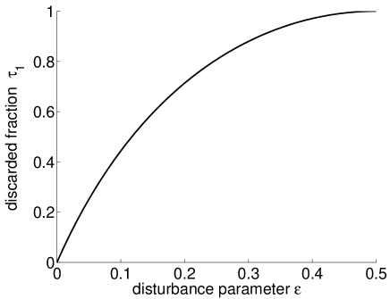
FIG. 2.: The fraction $\tau_{1}$ has to be discarded during privacy amplification as a function of the disturbance per correctly received element of the generalized sifted key if errors are discarded. This result is a sharp estimate in the sense that Eve can reach the level of collision probability on which the estimate is based.

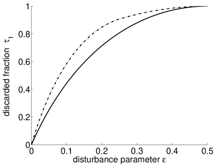
FIG. 3.: The fraction $\tau_{1}$ has to be discarded during privacy amplification as a function of the disturbance per element of the generalized sifted key if one corrects errors. If no information about the position of errors leaked to the eavesdropper, we find for $\tau_{1}$ the dash-dotted curve, for leaked error positions we find the solid curve.

Since we can not give an estimate for $\overline{\epsilon}$ from measured quantities the case of discarded errors, we concentrate on reconciliation methods which correct errors. From the results of this section we see that this is the better methods anyway, since discarding errors leads to a smaller $n_{\rm rec}$ than correcting errors. This number would have to be reduced further during privacy amplification than in the case of corrected errors, as can be seen by comparison of the estimates for $\tau_{1}$ as a function of $e$. Therefore the final key will be shorter and with that the protocol less efficient.

From the estimates we find that the direct estimate for $\tau_{1}$ gives higher values if the information about error positions has not leaked to the eavesdropper during reconciliation. We can regard the information of error positions as spoiling information [7] and thus use the estimate (85) even in the case of uni-lateral error correction. Spoiling information is any information which increases Eve’s Shannon information but decreases her expected collision probability on the key leading to a decreased value of $\tau_{1}$. We conclude that from the point of privacy amplification and reconciliation, the best known way to give a high rate of secure bits would be to use bi-lateral reconciliation methods.

V Analysis of the efficiency of key growing

The process of quantum key growing depends on physical parameters and on the security parameters of the final key. In this section we will bring together the essential formulas about the security statements concerning an accepted key and about the average key growing rate we can expect. This analysis is presented only for error correction reconciliation methods.

A Security needs

The first thing a potential user has to fix is the tolerated change of Shannon entropy $\Delta_{\rm tol}$ an eavesdropper might obtain on the key without posing a security hazard to the application in mind. Since this limit can not be guaranteed with absolute certainty, the user has to limit the tolerated probability $\alpha_{\rm tol}$ that Eve’s knowledge exceeds $\Delta_{\rm tol}$. Authentication may fail to detect errors leaving Alice and Bob with a key neither safe nor shared. The tolerated probability for this has to be specified as $\gamma_{\rm tol}$.

Given $I_{\rm tol}$, $\alpha_{\rm tol}$ and $\gamma_{\rm tol}$ and having in view a particular physical implementation of the quantum channel, Alice and Bob fix a value of the tolerated disturbance $\overline{\epsilon}_{\rm max}$ and of the security bits $n_{S}$ used in privacy amplification, as well as the length $n_{\rm sif}$ of the sifted key and the number of secure bits $N_{\rm aut}$ used for authentication such that for an accepted key the security target set by $I_{\rm tol},\alpha_{\rm tol}$ and $\gamma_{\rm tol}$ is met and that the rate of secure bits generated, given below, is optimized.

B Security statement

The following security statement holds if the key growing is performed by extracting a key of length

$$n_{\rm fin}=n_{\rm sif}\left[1-\tau_{1}(\overline{\epsilon}_{\rm max})\right]-n_{S}$$ (86)

from the reconciled key during privacy amplification. Here $\tau_{1}$ is given by by the functional dependence of equations (84) and (85) respectively. From the previous calculations we find that the bits generated in a run of the key growing process are secure in the sense that Eve achieves a change of Shannon entropy on the accepted key of less than $\Delta_{\rm tol}$ with probability $\alpha$. The contributions to $\alpha$ are the probability of failure of the estimation of the average disturbance given by $\alpha_{1}$ in equation (14), the probability to estimate the Shannon information in a specific run from the average information, given by $\alpha_{2}$ in equation (16) and the probability of faked authentication, given by $\alpha_{3}$ in equation (17). Since all those quantities are expected to be small, the estimate

$$\alpha \leq \alpha_{1}+\alpha_{2}+\alpha_{3}$$ (88)

$$=\exp(-2n_{\rm sif}\delta^{2})+\frac{\ln(2^{-n_{S}}+1)}{\Delta_{\rm tol}}+2^{-N_{\rm aut}+1}$$

$$\approx \exp(-2n_{\rm sif}\delta^{2})+\frac{2^{-n_{S}}}{\Delta_{\rm tol}\ln 2}+2^{-N_{\rm aut}+1}$$ (89)

with $\delta=\overline{\epsilon}_{\rm max}-\epsilon_{\rm meas}$ is sufficient for practical purposes.

The failure to establish a key in a specific run is due to the failure of authentication. Here two contributions can be distinguished. One is the failure of reconciliation, which happens with probability $\beta_{1}$, the other is the failure to reach the target of $\alpha_{\rm tol}$ in that run, which is signaled by making the authentication fail. This happens with a probability $\beta_{2}$. In the design of the set-up and the choice of parameters we would need to estimate $\beta$ so that at least in the absence of an eavesdropper we will find a net gain of secure bits according to the formula given below. Miscalculation of $\beta$ does not affect the security of the key, it only affects the efficiency of key generation. We omit therefore detailed examinations of values for $\beta$.

The last quantity concerning the security of the key is $\gamma$, which is the probability that authentication succeeds although Alice and Bob do not share a key. This probability can be estimated by $\gamma=2^{-N_{\rm aut}+1}$.

C Gain

In the previous subsection we described the influence of the chosen basic parameters on the acceptance and security of a run of key growing. Since we need secret bits as an input for the key generation we have to make sure that on average we will gain more secret bits than we put in. The important quantities are here the success probability $p_{\rm succ}=1-\beta$ that a run of the key expansion leads to accepted new secure bits, the number $N_{\rm out}=n_{\rm rec}\;[1-\tau_{1}(\overline{\epsilon}_{\rm max})]-n_{S}$ of secret bits gained in that instance and the average number $\overline{N}_{\rm in}=\overline{N}_{\rm rec}+N_{\rm aut}$ of input secret bits. Then the condition for an overall gain on average is to have a positive value of $\overline{N}_{\rm gain}=p_{\rm succ}N_{\rm out}-\overline{N}_{\rm in}$ resulting in

$$\overline{N}_{\rm gain} = (1-\beta)\left\{n_{\rm sif}\left[1-\tau_{1}(\overline{\epsilon}_{\rm max})\right]-n_{S}\right\}$$ (91)

$$-N_{\rm aut}-N_{\rm rec}\;.$$

To explore the implications of this condition we go to the limit of large sample sizes. Then we can neglect the number of secret bits used for authentication and and the safety parameter $n_{S}$. The remaining contribution of $\overline{N}_{\rm in}$ now comes from the error correction part. For ideal error correction we can set $\beta=0$ and can use the Shannon limit which gives $\overline{N}_{\rm in}=n_{\rm sif}(1-I_{AB}(\epsilon_{\rm meas}))$ with the Shannon information shared between Alice and Bob given by

$$I_{AB}(\epsilon_{\rm meas})=$$ (93)

$$1+\epsilon_{\rm meas}\log\epsilon_{\rm meas}+(1-\epsilon_{\rm meas})\log(1-\epsilon_{\rm meas})\;.$$

With these preparations we find

$$N_{\rm gain}=n_{\rm sif}\left[1-\tau_{1}(\epsilon_{\rm meas})\right]-n_{\rm sif}(1-I_{AB}(\epsilon_{\rm meas}))\;.$$

In the limit of $n_{\rm sif}\to\infty$ we can assume that $\delta\to 0$ still satisfies any confidence limits put on $\alpha$. Therefore the condition $\overline{N}_{\rm gain}\geq 0$ is now equivalent to

$$I_{AB}(\epsilon_{\rm meas})\geq\tau_{1}(\epsilon_{\rm meas})\;.$$ (94)

As we see from figure 4 this means that the protocol in the presented form will be able to grow secret keys only for set-ups operating at an error rate of less than $11.5\%$ for error correction. However, making use of the concept of spoiling information and of improved estimates of $p_{c}^{(1)}$ might result in lower estimates for $\tau_{1}$. A lower bound is, however, the Shannon information $I_{AE}$ shared by Alice and Eve in this scenario. Fuchs et al. give in [15] a sharp bound for $I_{AE}$, which is shown in figure 4 as dotted line. The difference between $\tau_{1}$ and $I_{AE}$ represent the average gain $G$ in a run of the key growing protocol in the limit of ideal error correction and infinite sample sizes. The gain

$$G=I_{AB}(\epsilon_{\rm meas})-\tau_{1}(\epsilon_{\rm meas})$$ (95)

gives the length of the final key as a fraction of the generalized sifted key.

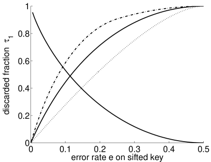
FIG. 4.: Shortening during privacy amplification, represented by $\tau_{1}$ (uni-lateral scenario in dash-dotted curve, bi-lateral scenario as solid curve), in balance with the loss during reconciliation, represented by $I_{AB}$ (falling solid line). The intersections between two lines limits the tolerable error rate in the generalized sifted key in the case of corrected errors. A lower limit of potentially improved bounds for $\tau_{1}$ is $I_{AE}$ (dotted line).

VI Concluding Remarks

In this paper I have given estimates needed in quantum cryptography which are closely oriented towards practical experiments. I do not deal with security against all possible attacks in quantum mechanics, but I deal with all attacks on individual signals. This allows me to include issues related to practical implementation of quantum cryptography which still can not be treated in the general scenario. One of these issues is the question of signals which, for example, triggered simultaneously two detectors monitoring orthogonal polarization modes. (This is the question of multi-photon signals resent by Eve, leading to ambiguous signals.) The other important question is that of an efficient key reconciliation prior to privacy amplification. As seen in this paper it is possible to use the efficient bi-lateral error correction scheme of Brassard and Salvail [14] without compromising security.

In the statistical analysis I showed that it is possible to limit in this scenario the knowledge of the eavesdropper on the final key in a individual realization from measured quantities for parameters which seem to be reachable in experiments. As measure of the eavesdropper’s knowledge I used the change between a-priori and a-posteriori Shannon entropy associated with the corresponding probability distributions over all possible keys from Eve’s point of view. One has to take into account that single photon signals states are not used in today’s experiments. However, this theory can be extended to signal states containing multi-photon components. A first approach for that is to estimate $p_{c}^{x}=1$ for each bit of the reconciled key on which Eve could have performed successfully a splitting operation with subsequent delayed measurement. Denote by $n_{m}$ the total number of these bits, then we need to reduce the key during privacy amplification by

$$\tau_{1}^{(mult)}(\overline{\epsilon})=\frac{n_{m}}{n_{\rm rec}}+\left(1-\frac{n_{m}}{n_{\rm rec}}\right)\tau_{1}\left(\overline{\epsilon}\frac{n_{\rm rec}}{n_{\rm rec}-n_{m}}\right)\;.$$ (96)

The statistics, however, becomes more complicated this way and it seems to be better to include the dim coherent states directly as signal states and to solve the problem in a clean way. Work in that direction is currently under progress.

The estimates for $\tau_{1}$ are not necessarily sharp in the case of error correction, and even in the case of discarding errors this limit could be lowered using spoiling information [7]. However, the possible improvement of efficiency of the key growing process is limited and this fine-tuning might be postponed until the experimental relevant situation for dim coherent signal states is solved.

A Cauchy inequality

In this appendix we prove the inequality (60) starting from the expression

$$p_{c}^{(1)} = \frac{1}{8p_{\rm rec}^{(1)}}\sum_{k\in K^{(1)}}\frac{(A^{k}_{00})^{4}+(A^{k}_{11})^{4}}{(A^{k}_{00})^{2}+(A^{k}_{11})^{2}}$$ (A2)

$$+\frac{1}{8p_{\rm rec}^{(1)}}\sum_{k^{\prime}\in K^{\prime(1)}}\frac{(\tilde{B}^{k^{\prime}}_{00})^{4}+(\tilde{B}^{k^{\prime}}_{11})^{4}}{(\tilde{B}^{k^{\prime}}_{00})^{2}+(\tilde{B}^{k^{\prime}}_{11})^{2}}\;.$$

We rewrite the first sum as

$$\sum_{k}\left((A^{k}_{00})^{2}+(A^{k}_{11})^{2}-2\frac{\left(A^{k}_{00}A^{k}_{11}\right)^{2}}{(A^{k}_{00})^{2}+(A^{k}_{11})^{2}}\right)\;$$ (A3)

and use the Cauchy inequality, given as

$$\left(\sum_{k}x_{k}y_{k}\right)^{2}\leq\left(\sum_{k}x_{k}^{2}\right)\left(\sum_{k}y_{k}^{2}\right)$$ (A4)

or

$$\sum_{k}x_{k}^{2}\geq\frac{\left(\sum_{k}x_{k}y_{k}\right)^{2}}{\sum_{k}y_{k}^{2}\;.}$$ (A5)

We set $x_{k}=\frac{\left(A^{k}_{00}A^{k}_{11}\right)}{\sqrt{(A^{k}_{00})^{2}+(A^{k}_{11})^{2}}}$ and $y_{k}=\sqrt{(A^{k}_{00})^{2}+(A^{k}_{11})^{2}}$ to obtain the inequality

$$\sum_{k}\frac{(A^{k}_{00})^{4}+(A^{k}_{11})^{4}}{(A^{k}_{00})^{2}+(A^{k}_{11})^{2}}\leq$$ (A7)

$$\sum_{k}\left((A^{k}_{00})^{2}+(A^{k}_{11})^{2}\right)-2\frac{\left(\sum_{k}A^{k}_{00}A^{k}_{11}\right)^{2}}{\sum_{k}(A^{k}_{00})^{2}+(A^{k}_{11})^{2}}\;.$$

This can be used to estimate the first part in (A2) while the second part can be estimated similarly so that, with the help of eqn. (57), we find the result

$$p_{c}^{(1)}\leq 1$$ (A9)

$$-\frac{1}{4p_{\rm rec}}\frac{\left({\bf A}_{00}{\bf A}_{11}\right)^{2}}{|{\bf A}_{00}|^{2}+|{\bf A}_{11}|^{2}}-\frac{1}{4p_{\rm rec}}\frac{\left({\bf\tilde{B}}_{00}{\bf\tilde{B}}_{11}\right)^{2}}{|{\bf\tilde{B}}_{00}|^{2}+|{\bf\tilde{B}}_{11}|^{2}}\;.$$

B Maximizing $p_{c}^{(1)}$ for discarded errors

To optimize the expression (60) we first note that we can assume that $|{\bf A}_{00}|=|{\bf A}_{11}|$. If Eve starts with a strategy defined by operators $A_{k}$ not satisfying this condition, then she could use the A-operators $\overline{A}_{k}=\left(\begin{array}[]{cc}0&1\\ 1&0\end{array}\right)A_{k}\left(\begin{array}[]{cc}0&1\\ 1&0\end{array}\right)$ without a change in the obtained collision probability or disturbance. When we combine the two strategies we find that the resulting vectors satisfy $|{\bf A}_{00}|=|{\bf A}_{11}|$ and $|{\bf A}_{01}|=|{\bf A}_{10}|$. This then gives the estimate $|{\bf A}_{01}+{\bf A}_{10}|^{2}\leq 4|{\bf A}_{01}|^{2}$. Another observation is that we can always choose $|{\bf A}_{00}|+|{\bf A}_{11}|\geq|{\bf\tilde{B}}_{00}|+|{\bf\tilde{B}}_{11}|$ which means that there are less or equal errors in the sifted key coming from the use of the polarization basis ’+’ than from the basis ’$\times$’. This can be always satisfied, since both polarization basis could be interchanged. Using $|{\bf A}_{00}|=|{\bf A}_{11}|$ and the definition of $|{\bf\tilde{B}}_{00}|$ and $|{\bf\tilde{B}}_{11}|$ this results in $2|{\bf A}_{00}|^{2}(1-\cos\phi_{00}^{11})\geq|{\bf A}_{01}+{\bf A}_{10}|^{2}$ with the angle $\phi_{00}^{11}$ between ${\bf A}_{00}$ and ${\bf A}_{11}$.

The three relevant relations now become after elimination of $p_{\rm rec}^{(1)}$ according to (43) and the use of the relations (49)

$$p_{c}^{(1)} \leq 1-\frac{(1+\overline{\epsilon}^{(1)})|{\bf A}_{00}|^{2}(\cos\phi_{00}^{11})^{2}}{8p_{\rm sif}}-\frac{(1+\overline{\epsilon}^{(1)})\left(2|{\bf A}_{00}|^{2}(1+\cos\phi_{00}^{11})-|{\bf A}_{01}+{\bf A}_{10}|^{2}\right)^{2}}{32p_{\rm sif}\left(2|{\bf A}_{00}|^{2}(1+\cos\phi_{00}^{11})+|{\bf A}_{01}+{\bf A}_{10}|^{2}\right)}$$ (B1)

$$\frac{p_{\rm sif}}{(1+\overline{\epsilon}^{(1)})} = \frac{1}{8}\left(|{\bf A}_{00}|^{2}(3+\cos\phi_{00}^{11})+\frac{1}{2}|{\bf A}_{01}+{\bf A}_{10}|^{2}\right)$$ (B2)

$$p_{\rm sif} = \frac{1}{2}\left(|{\bf A}_{00}|^{2}+|{\bf A}_{01}|^{2}\right)$$ (B3)

Our next step is to show that we can estimate the optimal value of $p_{c}^{(1)}$ by replacing $|{\bf A}_{01}+{\bf A}_{10}|^{2}$ by $4|{\bf A}_{01}|^{2}$. To see that we observe that this would allow to decrease $(1+\overline{\epsilon}^{(1)})$ by eqn (B2), meaning a lower error rate. At the same time $p_{c}^{(1)}$ grows indirectly from the falling value of $(1+\overline{\epsilon}^{(1)})$ and directly, since $\frac{d}{dD}p_{c}^{(1)}\geq 0$ with $D:=|{\bf A}_{01}+{\bf A}_{10}|^{2}$. To prove the last point we calculate

$$\frac{d}{dD}p_{c}^{(1)} = \frac{(1+\overline{\epsilon}^{(1)}){\cal A}}{32p_{\rm sif}\left(2|{\bf A}_{00}|^{2}+D+2|{\bf A}_{00}|^{2}\cos\phi_{00}^{11}\right)^{2}}$$ (B4)

$${\cal A} = 12|{\bf A}_{00}|^{4}-4|{\bf A}_{00}|^{2}D-D^{2}+24|{\bf A}_{00}|^{4}\cos\phi_{00}^{11}-4|{\bf A}_{00}|^{2}D\cos\phi_{00}^{11}+12|{\bf A}_{00}|^{4}(\cos\phi_{00}^{11})^{2}\;.$$ (B5)

This is positive, if ${\cal A}$ is positive. This is, indeed, the case since

$$\frac{d}{dD}{\cal A}=-4|{\bf A}_{00}|^{2}-2D-4|{\bf A}_{00}|^{2}\cos\phi_{00}^{11}\leq 0$$ (B6)

allows us to evaluate ${\cal A}$ at the maximal value of $D_{\rm max}=2|{\bf A}_{00}|^{2}(1-\cos\phi_{00}^{11})$ where it gives zero. This proves that ${\cal A}\geq 0$ and with that $\frac{d}{dD}p_{c}^{(1)}\geq 0$. Therefore, three relevant equations become

$$p_{c}^{(1)} \leq 1-\frac{(1+\overline{\epsilon}^{(1)})|{\bf A}_{00}|^{2}(\cos\phi_{00}^{11})^{2}}{8p_{\rm sif}}-\frac{(1+\overline{\epsilon}^{(1)})\left(|{\bf A}_{00}|^{2}(1+\cos\phi_{00}^{11})-2|{\bf A}_{01}|^{2}\right)^{2}}{16p_{\rm sif}\left(|{\bf A}_{00}|^{2}(1+\cos\phi_{00}^{11})+2|{\bf A}_{01}|^{2}\right)}$$ (B7)

$$\frac{p_{\rm sif}}{(1+\overline{\epsilon}^{(1)})} = \frac{1}{8}\left(|{\bf A}_{00}|^{2}(3+\cos\phi_{00}^{11})+2|{\bf A}_{01}|^{2}\right)$$ (B8)

$$p_{\rm sif} = \frac{1}{2}\left(|{\bf A}_{00}|^{2}+|{\bf A}_{01}|^{2}\right)$$ (B9)

We solve (B8) and (B9) for $|{\bf A}_{01}|$ and $\cos\phi_{00}^{11}$ and insert these into (B7). The maximum over $|{\bf A}_{00}|$ is then taken and we find

$$p_{c}^{(1)}\leq\frac{1}{2}\left(1+4\overline{\epsilon}^{(1)}-4\left(\overline{\epsilon}^{(1)}\right)^{2}\right)\;.$$ (B10)

The strategy resulting in this collision probability is described by

$$|{\bf A}_{00}|^{2} = |{\bf A}_{11}|^{2}=\frac{2p_{\rm sif}}{1+\overline{\epsilon}^{(1)}}$$ (B11)

$$|{\bf A}_{01}|^{2} = |{\bf A}_{10}|^{2}=\frac{2p_{\rm sif}\overline{\epsilon}^{(1)}}{1+\overline{\epsilon}^{(1)}}$$ (B12)

$$\cos\phi_{00}^{11} = 1-2\overline{\epsilon}^{(1)}$$ (B13)

$$\cos\phi_{01}^{10} = 1\;.$$ (B14)

In the derivation we have chosen $2|{\bf A}_{00}|^{2}(1-\cos\phi_{00}^{11})\geq|{\bf A}_{01}+{\bf A}_{10}|^{2}$ and find the optimal solution respects this choice for $\overline{\epsilon}^{(1)}\leq\frac{1}{2}$. For $\overline{\epsilon}^{(1)}=\frac{1}{2}$ we find $p_{c}^{(1)}=1$ so that we conclude that

$$p_{c}^{(1)}\leq\left\{\begin{array}[]{ll}\frac{1}{2}\left(1+4\overline{\epsilon}^{(1)}-4\left(\overline{\epsilon}^{(1)}\right)^{2}\right)&\mbox{for $\overline{\epsilon}^{(1)}\leq 1/2$}\\ 1&\mbox{for $\overline{\epsilon}^{(1)}\geq 1/2$}\end{array}\;.\right.$$ (B15)

C Maximizing $p_{c}^{(1)}$ for corrected errors

We start from equation (65) and use the Cauchy inequality in a similar way as in appendix B. We obtain the bound

$$p_{c}^{(1)} \leq 1-\frac{\left({\bf A}_{00}{\bf A}_{10}\right)^{2}+\left({\bf A}_{00}{\bf A}_{11}\right)^{2}+\left({\bf A}_{01}{\bf A}_{10}\right)^{2}+\left({\bf A}_{01}{\bf A}_{11}\right)^{2}}{\left(\left|{\bf A}_{00}\right|^{2}+\left|{\bf A}_{01}\right|^{2}+\left|{\bf A}_{10}\right|^{2}+\left|{\bf A}_{11}\right|^{2}\right)^{2}}$$ (C2)

$$-\frac{\left({\bf\tilde{B}}_{00}{\bf\tilde{B}}_{10}\right)^{2}+\left({\bf\tilde{B}}_{00}{\bf\tilde{B}}_{11}\right)^{2}+\left({\bf\tilde{B}}_{01}{\bf\tilde{B}}_{10}\right)^{2}+\left({\bf\tilde{B}}_{01}{\bf\tilde{B}}_{11}\right)^{2}}{\left(\left|{\bf\tilde{B}}_{00}\right|^{2}+\left|{\bf\tilde{B}}_{01}\right|^{2}+\left|{\bf\tilde{B}}_{10}\right|^{2}+\left|{\bf\tilde{B}}_{11}\right|^{2}\right)^{2}}\;.$$

Next we introduce the angles $\varphi_{00}^{11},\varphi_{00}^{10},\varphi_{01}^{10}$ between the corresponding vectors ${\bf A}_{00},{\bf A}_{10},{\bf A}_{01},{\bf A}_{11}$, make use of the relations (49) and (53), use the symmetry argument as in appendix B and find after some transformation the set of equations

$$p_{c}^{(1)}\leq\frac{3}{4}$$ (C5)

$$+\frac{\left|{\bf A}_{00}\right|^{4}(1-3\cos^{2}\varphi_{00}^{11})+\left|{\bf A}_{01}\right|^{4}(1-3\cos^{2}\varphi_{01}^{10})}{8(\left|{\bf A}_{00}\right|^{2}+\left|{\bf A}_{01}\right|^{2})^{2}}$$

$$+\left|{\bf A}_{00}\right|^{2}\left|{\bf A}_{01}\right|^{2}\frac{3+\cos\varphi_{00}^{11}\cos\varphi_{01}^{10}-2\cos^{2}\varphi_{00}^{10}}{4(\left|{\bf A}_{00}\right|^{2}+\left|{\bf A}_{01}\right|^{2})^{2}}$$

$$\overline{\epsilon}^{(1)} = \frac{\left|{\bf A}_{00}\right|^{2}(1-\cos\varphi_{00}^{11})+\left|{\bf A}_{01}\right|^{2}(3-\cos\varphi_{01}^{10})}{4(\left|{\bf A}_{00}\right|^{2}+\left|{\bf A}_{01}\right|^{2})}$$ (C6)

The first observation is that it is optimal to choose $\cos\varphi_{00}^{10}=0$ since this choice optimizes $p_{c}^{(1)}$ while it leaves $\overline{\epsilon}^{(1)}$ unchanged. The second observation is that the choice of

$$\left|{\bf A}_{00}\right|^{2}\cos\varphi_{00}^{11}=\left|{\bf A}_{01}\right|^{2}\cos\varphi_{01}^{10}$$ (C7)

within the subspace defined by

$$\left|{\bf A}_{00}\right|^{2}\cos\varphi_{00}^{11}+\left|{\bf A}_{01}\right|^{2}\cos\varphi_{01}^{10}=const$$

and fixed values of $\left|{\bf A}_{00}\right|$ and $\left|{\bf A}_{01}\right|$ is optimal if this choice is possible. In this case we are left with the equations

$$p_{c}^{(1)}\leq\frac{3}{4}$$ (C9)

$$+\frac{\left|{\bf A}_{00}\right|^{4}(1-4\cos^{2}\varphi_{00}^{11})+\left|{\bf A}_{01}\right|^{4}+6\left|{\bf A}_{00}\right|^{2}\left|{\bf A}_{01}\right|^{2}}{8(\left|{\bf A}_{00}\right|^{2}+\left|{\bf A}_{01}\right|^{2})^{2}}$$

$$\overline{\epsilon}^{(1)} = \frac{\left|{\bf A}_{00}\right|^{2}(1-2\cos\varphi_{00}^{11})+3\left|{\bf A}_{01}\right|^{2}}{4(\left|{\bf A}_{00}\right|^{2}+\left|{\bf A}_{01}\right|^{2})}\;.$$ (C10)

At the end of a short maximization calculation we find a solution consistent with symmetry condition (C7) for $\frac{1}{4}\leq\overline{\epsilon}^{(1)}\leq\frac{1}{2}$. It is given by

$$p_{c}^{(1)}\leq\frac{3}{4}+\overline{\epsilon}^{(1)}-\left(\overline{\epsilon}^{(1)}\right)^{2}\;.$$ (C11)

This maximum is obtained by choosing the values $\cos\varphi_{00}^{11}=\frac{1-2\overline{\epsilon}^{(1)}}{2(1-\overline{\epsilon}^{(1)})}$ and $\left|{\bf A}_{01}\right|=\left|{\bf A}_{00}\right|\sqrt{\frac{\overline{\epsilon}^{(1)}}{1-\overline{\epsilon}^{(1)}}}$. The symmetry condition (C7) then gives $\cos\varphi_{01}^{10}=\frac{1-2\overline{\epsilon}^{(1)}}{2\overline{\epsilon}^{(1)}}$ which limits the range of validity to $\frac{1}{4}\leq\overline{\epsilon}^{(1)}$. For $\frac{1}{4}\geq\overline{\epsilon}^{(1)}$ we find the optimal solution by selecting $\cos\varphi_{01}^{10}=1$. A short maximization calculation then gives the bound

$$p_{c}^{(1)}\leq\frac{1}{2}+3\overline{\epsilon}^{(1)}-5\left(\overline{\epsilon}^{(1)}\right)^{2}$$ (C12)

for the choice of parameters $\cos\varphi_{00}^{11}=\frac{1-3\overline{\epsilon}^{(1)}}{1-\overline{\epsilon}^{(1)}}$ and $\left|{\bf A}_{01}\right|=\left|{\bf A}_{00}\right|\sqrt{\frac{\overline{\epsilon}^{(1)}}{1-\overline{\epsilon}^{(1)}}}$.

D Maximizing $p_{c}^{(1)}$ for corrected errors with leaked error positions

We apply Cauchy inequalities to equation (75) and use the vector notations ${\bf A}$, ${\bf\tilde{B}}$, ${\bf C}$, and ${\bf\tilde{D}}$ to find

$$p_{c}^{(1)}\leq 1$$ (D3)

$$-\frac{1}{4p_{\rm sif}}\frac{\left|{\bf A}_{00}{\bf A}_{11}\right|^{2}}{|{\bf A}_{00}|^{2}+|{\bf A}_{11}|^{2}}-\frac{1}{4p_{\rm sif}}\frac{\left|{\bf C}_{01}{\bf C}_{10}\right|^{2}}{|{\bf C}_{01}|^{2}+|{\bf C}_{10}|^{2}}$$

$$-\frac{1}{4p_{\rm sif}}\frac{\left|{\bf\tilde{B}}_{00}{\bf\tilde{B}}_{11}\right|^{2}}{|{\bf\tilde{B}}_{00}|^{2}+|{\bf\tilde{B}}_{11}|^{2}}-\frac{1}{4p_{\rm sif}}\frac{\left|{\bf\tilde{D}}_{01}{\bf\tilde{D}}_{10}\right|^{2}}{|{\bf\tilde{D}}_{01}|^{2}+|{\bf\tilde{D}}_{10}|^{2}}\;.$$

It becomes clear immediately that we can replace ${\bf C}$ by ${\bf A}$ and ${\bf\tilde{D}}$ by ${\bf\tilde{B}}$ because of relations similar to (53). Similar to the calculations in appendices B and C we introduce the angles $\varphi_{00}^{11},\varphi_{00}^{10},\varphi_{01}^{10}$ and use the relations (49) and (53) and the symmetry argument introduced in appendix B to find the new form of (D3) as

$$p_{c}^{(1)} \leq \frac{3}{4}-\frac{|{\bf A}_{00}|^{2}\cos^{2}\varphi_{00}^{11}+|{\bf A}_{01}|^{2}\cos^{2}\varphi_{01}^{10}}{4(|{\bf A}_{00}|^{2}+|{\bf A}_{01}|^{2})}$$ (D6)

$$+\frac{|{\bf A}_{00}|^{2}|{\bf A}_{01}|^{2}}{2(|{\bf A}_{00}|^{2}+|{\bf A}_{01}|^{2})}\left[\frac{(1+\cos\varphi_{00}^{11})(1+\cos\varphi_{01}^{10})}{|{\bf A}_{00}|^{2}(1+\cos\varphi_{00}^{11})+|{\bf A}_{01}|^{2}(1+\cos\varphi_{01}^{10})}+\right.$$

$$\mbox{\hskip 56.9055pt}\left.\frac{(1-\cos\varphi_{00}^{11})(1-\cos\varphi_{01}^{10})}{|{\bf A}_{00}|^{2}(1-\cos\varphi_{00}^{11})+|{\bf A}_{01}|^{2}(1-\cos\varphi_{01}^{10})}\right]$$

while we take from appendix C the expression for $\overline{\epsilon}^{(1)}$ as

$$\overline{\epsilon}^{(1)}=\frac{\left|{\bf A}_{00}\right|^{2}(1-\cos\varphi_{00}^{11})+\left|{\bf A}_{01}\right|^{2}(3-\cos\varphi_{01}^{10})}{4(\left|{\bf A}_{00}\right|^{2}+\left|{\bf A}_{01}\right|^{2})}\;.$$ (D7)

We next perform a variation along the path defined by $\left|{\bf A}_{00}\right|^{2}\cos\varphi_{00}^{11}+\left|{\bf A}_{01}\right|^{2}\cos\varphi_{01}^{10}=const$ and find that $p_{c}^{(1)}$ is optimized for the choice $\cos\varphi_{00}^{11}=\cos\varphi_{01}^{10}$. An optimization calculation for the remaining parameters leads to the estimate

$$p_{c}^{(1)}\leq\frac{1}{2}+2\overline{\epsilon}^{(1)}-2\left(\overline{\epsilon}^{(1)}\right)^{2}$$ (D8)

for a disturbance $\overline{\epsilon}^{(1)}\leq 1/2$. This optimum is obtained by choosing $\cos\varphi_{00}^{11}=1-2\overline{\epsilon}^{(1)}$ and $|{\bf A}_{00}|=|{\bf A}_{01}|\sqrt{\frac{1-\overline{\epsilon}^{(1)}}{\overline{\epsilon}^{(1)}}}$.

REFERENCES

- [1] C. H. Bennett and G. Brassard, In Proceedings of IEEE International Conference on Computers, Systems, and Signal Processing, Bangalore, India, (IEEE, New York, 1984) pp. 175–179.
- [2] B. Huttner and A. K. Ekert, J. Mod. Opt. 41, 2455–2466 (1994).
- [3] C. Marand and P. T. Townsend, Opt. Lett. 20, 1695–1697 (1995).
- [4] H. Zbinden, N. Gisin, B. Huttner, A. Muller, J. Cryptol. 11, 1–14 (1998).
- [5] J. D. Franson and H. Ilves, J. Mod. Opt. 41, 2391–2396 (1994).
- [6] W. T. Buttler, R. J. Hughes, P. G. Kwiat, G. G. Luther, G. L. Morgan, J. E. Nordholt, C. G. Peterson, and C. M. Simmons, Phys. Rev. A 57, 2379–2382 (1998).
- [7] C. H. Bennett, G. Brassard, C. Crépeau, and U. M. Maurer, IEEE Trans. Inf. Theo. 41, 1915 (1995).
- [8] C. K. Law and H. J. Kimble, J. Mod. Opt. 44, 2067–2074 (1997).
- [9] H. P. Yuen, Quantum. Semicl. Opt. 8, 939–949 (1996).
- [10] B. Huttner and N. Imoto and N. Gisin and T. Mor, Phys. Rev. A 51, 1863–1869 (1995).
- [11] D. Mayers, Report quant-ph/9802025, (1998).
- [12] E. Biham, M. Boyer, G. Brassard, J. van de Graaf, and T. Mor, Report quant-ph/9801022, (1998).
- [13] C. Cachin and U. M. Maurer, J. Crypt. 10, 97–110 (1997).
- [14] G. Brassard and L. Salvail, In Proceedings of Eurocrypt ’93, held in Lofthus, Norway, 1993,
- [15] C. A. Fuchs, N. Gisin, R. B. Griffiths, C.-S. Niu, and A. Peres, Phys. Rev. A 56, 1163–1176 (1997).
- [16] N. Lütkenhaus, Phys. Rev. A 54, 97 (1996).
- [17] W. Hoeffding, J. Amer. Stat. Ass 58, 13–30 (1963).
- [18] In an earlier version of this paper I omitted the authentication of this step. I am grateful to Miloslav Dušek for pointed out to me the danger arising from that.
- [19] M. N. Wegman and J. L. Carter, J. Comp. Syst. Sci. 22, 265–279 (1981).
- [20] E. B. Davies, Quantum Theory of Open Systems (Academic Press, London, New York, San Francisco, 1976).
- [21] K. Kraus, in States, Effects, and Operations, No. 190 in Lecture Notes in Physics, A. Böhm, J. D. Dollard, and W. Wooters, eds., (Springer, Berlin, 1983).
- [22] B. Yurke, Phys. Rev. A 32, 311–323 (1985).
- [23] N. Lütkenhaus, Ph.D. thesis, University of Strathclyde, Glasgow, Scotland, 1996.
- [24] N. Lütkenhaus and S. M. Barnett, In Proceedings of an International Workshop on Quantum Communication, Computing, and Measurement, held September 25-30 in Shizuoka, Japan, O. Hirota, A. S. Holevo, and C. M. Caves, eds., (Plenum Press, New York, 1997).
- [25] B. Slutsky, P. C. Sun, Y. Mazurenko, R. Rao, and Y. Fainman, J. Mod. Opt. 44, 953–961 (1997).
- [26] B. Slutsky, R. Rao, P. C. Sun, and Y. Fainman, Phys. Rev. A 57, 2383–2398 (1998).