Optimal Copying of One Quantum Bit

Abstract

A quantum copying machine producing two (in general non-identical) copies of an arbitrary input state of a two-dimensional Hilbert space (qubit) is studied using a quality measure based on distinguishability of states, rather than fidelity. The problem of producing optimal copies is investigated with the help of a Bloch sphere representation, and shown to have a well-defined solution, including cases in which the two copies have unequal quality, or the quality depends upon the input state (is “anisotropic” in Bloch sphere language), or both. A simple quantum circuit yields the optimal copying machine. With a suitable choice of parameters it becomes an optimal eavesdropping machine for some versions of quantum cryptography, or reproduces the Bužek and Hillery result for isotropic copies.

I Introduction

The no-cloning theorem [1, 2] is one of the most important features which distinguishes quantum from classical information theories. There is no difficulty making an arbitrary number of copies of any type of information which arrives over a classical channel. However, to copy or “clone” the information which arrives over a quantum channel is not possible without producing errors if it is encoded in terms of nonorthogonal quantum states. This fact is the basis for various schemes of quantum cryptography [3], since the attempt of an eavesdropper to tap into a quantum channel and duplicate the information in it will result in errors detectable by the legitimate users.

Even in cases in which perfect copies are excluded because of the no-cloning theorem, it is possible to produce imperfect copies which are better than random noise. An optimal copying machine is one in which, by means of a suitable unitary transformation, a certain number of copies of the original information are produced with the smallest number of errors, or minimal amount of noise. Optimality in this sense will obviously depend upon the ensemble of input states, the number of copies, and the measure employed for noise or error rate. Obtaining quantitative estimates of what is possible for optimal copying is a significant problem in quantum information theory, and it is to this problem that the present paper is addressed.

A number of previous studies have used various input ensembles and measures of quality or of noise. Bužek and Hillery discussed an “isotropic”, or “universal”, copying machine [4], which produces two identical copies from one qubit (two-state system), with copy quality independent of the input state. This copying machine was later proved by Bruß et al. [5] to be optimal among all possible isotropic machines, if the measure of quality is the fidelity between the input and the output: that is, the probability that the output will be measured to be in the same state as the input. Gisin and Massar [6] considered a case in which $M$ identical copies are generated from $N$ identical qubits $(M>N)$, and found that the average fidelity reaches its maximum when the machine is isotropic. Bruß, Ekert, and Macchiavello [7] found an interesting connection between the optimal isotropic copying process and quantum state estimation by measurement. Later, the optimal $M$-to-$N$ problem was generalized by Werner [8] to systems of arbitrary dimension. Various quantum circuits implementing some of the isotropic copying machines mentioned above are presented in [9, 10]. Brußet al. [5] also considered an input ensemble of two non-orthogonal states, and found that the optimal copying process requires no ancillary qubits, unlike the case of isotropic copying.

In contrast to the work just discussed, we will use a quality measure based upon the distinguishability of the output states, rather than the fidelity, and will consider non-identical and anisotropic copies for which the copying quality can depend upon the input state. This is motivated by a study of eavesdropping in quantum cryptography [11]. Eavesdropping is, in essence, a matter of producing imperfect “copies” of the input signal in some channel in a way which enables the eavesdropper to distinguish the different states in the original information, while at the same time perturbing it as little as possible. Thus distinguishability is more important to the eavesdropper than whether his copies resemble the original states. In addition, the amount of information obtained by the legitimate receiver and by the eavesdropper are generally different, and can depend on the input states. Since the problem of optimizing a copy machine for completely general inputs and outputs is quite difficult, we restrict ourselves to the case of only two copies of one qubit. Even with this restriction, the mathematical structure is nontrivial. Recently Cerf [12] explored this problem by investigating a family of “Pauli cloning machines.” He derived a no-cloning inequality for isotropic copies, and established a bound for the quantum capacity of the corresponding “Pauli channel.”

We introduce the background material needed for later sections in Sec. II, including a formalism for the general interaction of one qubit with another quantum system, a set of superoperators, and the Bloch sphere representation. In Sec. III, the quality function of an output qubit is defined, and it is expressed using the Bloch sphere representation; this is the measure we employ to define optimal copying. Given the quality of one copy, the best quality for the other is determined by a map $G$, which is derived in Sec. IV for a special case. However, this special case is as good or better than any other copying scheme, as shown in Sec. V. Section VI discusses a number of properties of the map $G$, the conditions under which a pair of copies produced are actually optimal, and particular examples that are useful in revealing relations between the copying qualities. In Sec. VII we introduce two quantum circuits implementing the optimal copying process, and show how they can be turned into an eavesdropping machine or a universal copying machine. Finally, the results are summarized and some open questions are noted in Sec. VIII. Various mathematical details are placed in Appendices A–D.

II General formulation of the copying problem

We define the copying problem in the following way. The qubit which is to be copied is a state in a two-dimensional Hilbert space ${\cal A}$ with orthogonal basis $|0{\rangle}$ and $|1{\rangle}$. The copy machine corresponds to a unitary transformation $U$ on

$${\cal H}={\cal A}\otimes{\cal E}={\cal B}\otimes{\cal E}\ ={\cal B}\otimes{\cal C}\otimes{\cal D},$$ (1)

where we suppose that the copies lie in the two dimensional spaces ${\cal B}$ and ${\cal C}$ after the action of $U$, and the space ${\cal E}={\cal C}\otimes{\cal D}$ can have an arbitrarily large but finite (even) dimension. The identical spaces ${\cal A}$ and ${\cal B}$ are denoted differently in order to distinguish the input space from the output. In particular,

$$U(|j{\rangle}\otimes|\epsilon{\rangle})=\sum_{l=0}^{1}|l{\rangle}\otimes|\epsilon^{j}_{l}{\rangle},$$ (2)

where $|\epsilon{\rangle}$ is a normalized state of ${\cal E}$, and therefore the states $|\epsilon^{j}_{l}{\rangle}$ of ${\cal E}$ satisfy

$$\sum_{l}{\langle}\epsilon^{j}_{l}|\epsilon^{k}_{l}{\rangle}=\delta_{jk}.$$ (3)

There is no loss of generality in assuming a pure state $|\epsilon{\rangle}$ rather than a density matrix for ${\cal E}$, since a density matrix can always be thought of as arising from a partial trace on a space of higher dimension, and the dimension of ${\cal E}$ is arbitrary.

With $|\epsilon{\rangle}$ fixed, define the linear map $V:{\cal A}{\rightarrow}{\cal B}\otimes{\cal E}$ through

$$V|\alpha{\rangle}=U(|\alpha{\rangle}\otimes|\epsilon{\rangle})=\sum_{l=0}^{3}(\sigma_{l}|\alpha{\rangle})\otimes|e_{l}{\rangle},$$ (4)

where $\sigma_{0}$ is the identity, and $\sigma_{1}$, $\sigma_{2}$, and $\sigma_{3}$ are the usual Pauli matrices $\sigma_{x}$, $\sigma_{y}$, and $\sigma_{z}$, which in (4) should be thought of as maps from ${\cal A}$ to ${\cal B}$, assuming some basis $|0{\rangle},\,|1{\rangle}$ for the latter; here $|0{\rangle}$ and $|1{\rangle}$ correspond to $S_{z}$ equal to $+1/2$ and $-1/2$, respectively, and $(|0{\rangle}+|1{\rangle})/\sqrt{2}$ to $S_{x}=+1/2$ in the usual spin half notation. Thus if (4) is written out explicitly, it takes the form:

$$V|0{\rangle} = |0{\rangle}|e_{0}{\rangle}+|1{\rangle}|e_{1}{\rangle}+i|1{\rangle}|e_{2}{\rangle}+|0{\rangle}|e_{3}{\rangle},$$ (5)

$$V|1{\rangle} = |1{\rangle}|e_{0}{\rangle}+|0{\rangle}|e_{1}{\rangle}-i|0{\rangle}|e_{2}{\rangle}-|1{\rangle}|e_{3}{\rangle},$$ (6)

where, following the usual convention, we omit $\otimes$ if this causes no confusion. The four $|e_{l}{\rangle}$ are vectors in ${\cal E}$ which are linear combinations of the $|\epsilon^{j}_{k}{\rangle}$, and whose inner products form a $4\times 4$ positive (i.e., non-negative eigenvalues) Hermitian matrix $E$:

$$E_{lm}={\langle}e_{l}|e_{m}{\rangle}=E^{*}_{ml}.$$ (7)

Note that given a positive Hermitian matrix $E$, it is always possible to find a set of four vectors $|e_{l}{\rangle}$ such that $E_{lm}$ takes the form (7), and this set is unique up to an arbitrary unitary transformation on ${\cal E}$.

The condition (3) implied by the unitarity of $U$ is equivalent to the requirement that $V$ be an isometry, or that

$$V^{\dagger}V=\sum_{lm}E_{lm}\sigma_{l}\sigma_{m}=\sigma_{0},$$ (8)

the identity on ${\cal A}$, and thus to

$$\sum_{l=0}^{3}E_{ll} = 1,$$ (9)

$$\hbox{Re}(E_{0q}) = \hbox{Im}(E_{q^{\prime}q^{\prime\prime}}),$$ (10)

where Re and Im refer to real and imaginary parts, and (10) employs a notation which we will use again and again:

$$(q,q^{\prime},q^{\prime\prime})=(1,2,3)\mbox{ or }(2,3,1)\mbox{ or }(3,1,2).$$ (11)

That is, the triple $(q,q^{\prime},q^{\prime\prime})$ is an even permutation of the integers 1, 2, and 3. Thus, for example, $\hbox{Re}[E_{02}]=\hbox{Im}[E_{31}].$

Given $V$, the corresponding superoperator $\hat{V}$ which maps operators on ${\cal A}$ to operators on ${\cal H}$ takes the form

$$\hat{V}(\kappa)=V\kappa V^{\dagger}=\sum_{jk}\sigma_{j}\kappa\sigma_{k}\otimes|e_{j}{\rangle}{\langle}e_{k}|.$$ (12)

In particular, for $l=0,1,2,3,$

$$\hat{V}(\sigma_{l})=\sum_{jkm}L(jk;lm)\,\sigma_{m}\otimes|e_{j}{\rangle}{\langle}e_{k}|=\sum_{m}\sigma_{m}\otimes\hat{F}_{lm},$$ (13)

where the $\hat{F}_{lm}$ are a collection of 16 Hermitian operators on ${\cal E}$ defined by

$$\hat{F}_{lm}=\sum_{jk}L(jk;lm)\,|e_{j}{\rangle}{\langle}e_{k}|,$$ (14)

and

$$L(jk;lm)={\textstyle{1\over 2}}\hbox{Tr}[\sigma_{j}\sigma_{l}\sigma_{k}\sigma_{m}]$$ (15)

can be thought of as a $16\times 16$ matrix, with rows labeled by $jk$ and columns by $lm$. Its properties are discussed in App. A. In particular, ${\textstyle{1\over 2}}L$ is its own inverse. When $j=k$ or when $l=m$, $L(jk;lm)$ vanishes unless the other pair is also equal:

$$L(jk;ll)=\delta_{jk}\Lambda(j,l),\quad L(jj,lm)=\delta_{lm}\Lambda(j,l),$$ (16)

where $\Lambda(j,l)$ is a $4\times 4$ real matrix, (A8), whose square is 4 times the identity.

The superoperators $\hat{V}_{\cal B},$ $\hat{V}_{\cal C}$, and $\hat{V}_{\cal E}$, which play a central role in the following discussion, map operators on ${\cal A}$ to operators on ${\cal B}$, ${\cal C}$, and ${\cal E}$, respectively and are defined using partial traces of $\hat{V}$:

$$\hat{V}_{\cal B}(\kappa)=\hbox{Tr}_{\cal E}[\hat{V}(\kappa)],\quad\hat{V}_{\cal E}(\kappa)=\hbox{Tr}_{\cal B}[\hat{V}(\kappa)],$$ (17)

$$\hat{V}_{\cal C}(\kappa)=\hbox{Tr}_{{\cal B}\otimes{\cal D}}[\hat{V}(\kappa)]=\hbox{Tr}_{\cal D}[\hat{V}_{\cal E}(\kappa)]$$ (18)

The isometry condition (8) implies that $\hat{V}$ preserves the trace,

$$\hbox{Tr}_{\cal H}[\hat{V}(\kappa)]=\hbox{Tr}_{\cal A}[\kappa],$$ (19)

and this property is inherited by each of the superoperators $\hat{V}_{\cal B},$ $\hat{V}_{\cal C}$, and $\hat{V}_{\cal E}$, with the trace over ${\cal H}$ in (19) replaced by a trace over ${\cal B}$, ${\cal C}$, and ${\cal E}$, respectively. (Henceforth we shall not always indicate explicitly the space over which a trace is to be taken if it is obvious from the context.) In addition, it is obvious from (12) that $\hat{V}$ maps Hermitian operators to Hermitian operators, and this property is also inherited by $\hat{V}_{\cal B},$ $\hat{V}_{\cal C}$, and $\hat{V}_{\cal E}$.

It is convenient to write

$$\hat{V}_{\cal B}(\sigma_{l})=\sum_{m}B_{lm}\sigma_{m},$$ (20)

where

$$B_{lm}=\hbox{Tr}_{\cal E}[\hat{F}_{lm}]=\sum_{jk}L(lm;jk)\,E_{jk}$$ (21)

is a real $4\times 4$ matrix of the form:

$$B=\left(\matrix{1&\delta^{B}_{1}&\delta^{B}_{2}&\delta^{B}_{3}\cr 0&&&\cr 0&&\mbox{\boldmath$B$}&\cr 0&&&}\right),$$ (22)

where columns and rows are in the order $0,1,2,3$, and $B$ is a real $3\times 3$ matrix. The form of the first (left-most) column of $B$ is equivalent to the isometry condition (8), that is, to (9) plus (10), as can be shown by inserting in (21) the matrix elements for the $L$ given in App. A. It implies that the superoperator in (20) preserves the trace. The inverse of (21), see (A10), is

$$E_{jk}={\textstyle{1\over 4}}\sum_{lm}L(jk;lm)\,B_{lm}.$$ (23)

The vector $\mbox{\boldmath$\delta$}^{B}=(\delta^{B}_{1},\delta^{B}_{2},\delta^{B}_{3})$ and the matrix $B$ in (22) can be given a geometrical interpretation using the well-known Bloch sphere representation

$$\rho={\textstyle{1\over 2}}(I+\mbox{\boldmath$r\cdot\sigma$})={\textstyle{1\over 2}}(\sigma_{0}+\sum_{j=1}^{3}r_{j}\sigma_{j})$$ (24)

of a density matrix $\rho$ in a two-dimensional Hilbert space, where $\mbox{\boldmath$r$}=(r_{1},r_{2},r_{3})$ is any real vector of length less than 1 for a mixed state, or equal to 1 for a pure state, and $\mbox{\boldmath$\sigma$}=(\sigma_{1},\sigma_{2},\sigma_{3})$. Then (20) and (22) tell us that

$$\hat{V}_{\cal B}(\rho)=\rho^{\prime}={\textstyle{1\over 2}}(\sigma_{0}+\mbox{\boldmath$s\cdot\sigma$}),$$ (25)

where [13]

$$\mbox{\boldmath$s$}=\mbox{\boldmath$\delta$}^{B}+\mbox{\boldmath$r\cdot B$}=\mbox{\boldmath$\delta$}^{B}+\mbox{\boldmath$B^{\top}\cdot r$},$$ (26)

and $B^{\top}$ is the transpose of $B$. In particular, if (26) is applied to the collection of pure states, $|\mbox{\boldmath$r$}|=1$, which form the unit Bloch sphere of ${\cal A}$, the resulting collection of $s$ vectors forms an ellipsoid in the Bloch sphere of ${\cal B}$, which we shall call the ${\cal B}$ ellipsoid, or simply ellipsoid, with center at $\mbox{\boldmath$\delta$}^{B}$.

The polar decomposition [14] of $B$ takes the form

$$\mbox{\boldmath$B$}=\mbox{\boldmath$P\cdot B^{s}$},$$ (27)

where $P$ is a proper rotation, a real orthogonal $3\times 3$ matrix with determinant 1, and $B^{s}$ is a real symmetric matrix. By diagonalizing $B^{s}$, one can always write $B$ in the form

$$\mbox{\boldmath$B$}=\mbox{\boldmath$P^{\prime}\cdot B^{d}\cdot P^{\prime\prime}$},$$ (28)

where $P^{\prime}$ and $P^{\prime\prime}$ are proper rotations, and $B^{d}$ is a diagonal matrix with (real) eigenvalues $b_{1},b_{2},b_{3}$. The rotations $P^{\prime}$ and $P^{\prime\prime}$ correspond to unitary transformations on ${\cal A}$ and ${\cal B}$, respectively. Consequently, by adopting suitable orthonormal bases for ${\cal A}$ and ${\cal B}$, we can, assuming $U$ to be given, always arrange to have the matrix $B$ in the form

$$B=\left(\matrix{1&\delta^{B}_{1}&\delta^{B}_{2}&\delta^{B}_{3}\cr 0&b_{1}&0&0\cr 0&0&b_{2}&0\cr 0&0&0&b_{3}}\right),$$ (29)

parameterized by $\mbox{\boldmath$\delta$}^{B}=(\delta^{B}_{1},\delta^{B}_{2},\delta^{B}_{3})$ and $\mbox{\boldmath$b$}=(b_{1},b_{2},b_{3})$. (Note that in the process of diagonalizing the general form (22) to obtain the diagonal form (29), the values of the $\delta^{B}_{j}$ will, in general, change.)

Two vectors corresponding to an orthonormal basis or mode for ${\cal A}$ are represented by opposite poles $\mbox{\boldmath$\hat{m}$}=(m_{1},m_{2},m_{3})$ and $-\mbox{\boldmath$\hat{m}$}$ of the Bloch sphere of ${\cal A}$, where we use a hat to indicate a unit vector. Under (26) these map to opposite points of the ${\cal B}$ ellipsoid; that is, the line connecting them passes through the center $\mbox{\boldmath$\delta$}^{B}$ of the ellipsoid. The three principal axes of the ${\cal B}$ ellipsoid correspond to three principal modes of ${\cal A}$, represented in the Bloch sphere of ${\cal A}$ by mutually perpendicular unit vectors (and their negations) $\mbox{\boldmath$\hat{M}$}_{1}$, $\mbox{\boldmath$\hat{M}$}_{2}$, and $\mbox{\boldmath$\hat{M}$}_{3}$. If bases are chosen such that $B$ has the form (29), the mode vectors $\mbox{\boldmath$\hat{M}$}_{j}$ are along the Cartesian axes, and correspond, in the language of spin half, to a value of $+1/2$ for $S_{x}$, $S_{y}$, and $S_{z}$, respectively. (It is, of course, important to distinguish “orthogonal” with reference to the complex Hilbert spaces ${\cal A}$ or ${\cal B}$, from “perpendicular” as it refers to real three-dimensional vectors in the Bloch sphere representation!) Also, $|b_{j}|$ is the length of the $j^{\prime}$th principal semi-axis of the ellipsoid.

Because $P^{\prime}$ and $P^{\prime\prime}$ are proper rotations (each has determinant 1), it is not always possible to make all the $b_{j}$, $j=1,2,3$, in (29) positive (non-negative). If an even number of the $b_{j}$ are negative, then $P^{\prime}$ and $P^{\prime\prime}$ can be chosen so they are all positive, but if an odd number are negative, the best one can do is to have two positive and one negative. Which of these situations occurs depends upon $U$, and turns out to be of some significance for optimal copying.

Since ${\cal C}$ is also a two-dimensional space, we can use a Bloch sphere representation for $\hat{V}_{\cal C}$ and write the counterpart of (25) as

$$\hat{V}_{\cal C}(\rho)=\rho^{\prime\prime}={\textstyle{1\over 2}}(\sigma_{0}+\mbox{\boldmath$t\cdot\sigma$}),$$ (30)

where

$$\mbox{\boldmath$t$}=\mbox{\boldmath$\delta$}^{C}+\mbox{\boldmath$r\cdot C$}=\mbox{\boldmath$\delta$}^{C}+\mbox{\boldmath$C^{\top}\cdot r$}.$$ (31)

The counterpart of (22) is a $4\times 4$ matrix

$$C=\left(\matrix{1&\delta^{C}_{1}&\delta^{C}_{2}&\delta^{C}_{3}\cr 0&&&\cr 0&&\mbox{\boldmath$C$}&\cr 0&&&}\right),$$ (32)

where $C$ is a $3\times 3$ matrix which can be diagonalized by the same strategy employed earlier in the case of $B$, though the principal modes of ${\cal A}$ singled out by this construction will, in general, not be the same as those corresponding to the ${\cal B}$ ellipsoid, so we label the perpendicular unit vectors with a prime: $\mbox{\boldmath$\hat{M}$}^{\prime}_{1}$, $\mbox{\boldmath$\hat{M}$}^{\prime}_{2}$, and $\mbox{\boldmath$\hat{M}$}^{\prime}_{3}$. We shall denote by $\mbox{\boldmath$c$}=(c_{1},c_{2},c_{3})$ the values on the diagonal when $C$ is diagonalized; hence $|c_{j}|$ is the length of the $j^{\prime}$th principal semi-axis of the ${\cal C}$ ellipsoid.

The possible values of $b$ and $\mbox{\boldmath$\delta$}^{B}$ are constrained by the fact that, whatever $U$ may be, the matrix $E$, which determines $B$ through (21), and is determined by $B$ through the inverse relationship (23), satisfies the isometry condition (9) and (10) and has non-negative eigenvalues. One consequence is the fact that the ${\cal B}$ ellipsoid must always lie inside the unit Bloch sphere of ${\cal B}$. These constraints are found explicity for the case $\mbox{\boldmath$\delta$}^{B}=\mbox{\boldmath$0$}$ in Sec. IV below, but we do not know their form in general. There are, of course, identical constraints on the possible values of $c$ and $\mbox{\boldmath$\delta$}^{C}$

III Error rates and quality function

Consider the problem of a general channel of the type introduced in Sec. II, from a qubit ${\cal A}$ to a Hilbert space ${\cal F}$ (which could be ${\cal B}$ or ${\cal C}$ or ${\cal E}$), described by a superoperator $\hat{V}_{\cal F}$. Suppose that symbols $a_{1}$ and $a_{2}$ are encoded in basis states $\hat{m}$ and $-\mbox{\boldmath$\hat{m}$}$ in the Bloch sphere representation of ${\cal A}$, and the corresponding states are mapped by $\hat{V}_{\cal F}$ to the two density matrices $\rho_{\cal F}^{1}$ and $\rho_{\cal F}^{2}$ in ${\cal F}$. Now suppose that every time a signal $a_{1}$ or $a_{2}$ is sent, a measurement is carried out on ${\cal F}$ corresponding to a decomposition of the identity

$$I_{\cal F}=\sum_{k}F_{k},$$ (33)

where the $\{F_{k}\}$ are projectors, or, more generally, positive operators [15]. Further suppose that if the result of this measurement is $f_{k}$ corresponding to $F_{k}$, an estimate of the original symbol is made according to a fixed guessing function $g(a_{j}|f_{k})$ which is either 0 or 1, and satisfies

$$\sum_{j}g(a_{j}|f_{k})=1.$$ (34)

That is, if $g(a_{2}|f_{1})=1$, then if $f_{1}$ is measured, one guesses that $a_{2}$ was sent. If $a_{j}$ is sent with probability $p_{j}$, one can show that the average error rate (guessing $a_{1}$ when $a_{2}$ was sent, or vice versa) using this procedure is bounded below, see [16], by the (achievable) minimum error rate

$$\epsilon_{min}={\textstyle{1\over 2}}\left[1-\hbox{Tr}\Bigl{(}|p_{1}\rho_{\cal F}^{1}-p_{2}\rho_{\cal F}^{2}|\Bigr{)}\right],$$ (35)

where the absolute value $|C|$ of a Hermitian operator $C$ is the operator obtained by replacing the eigenvalues of $C$ with their absolute values in its spectral decomposition. Motivated by (35), we define the quality factor ${\cal Q}_{\cal F}(\mbox{\boldmath$\hat{m}$})$ or “distinguishability” for mode $\hat{m}$ as

$${\cal Q}_{\cal F}(\mbox{\boldmath$\hat{m}$})={\textstyle{1\over 2}}\hbox{Tr}\left(|\rho_{\cal F}^{1}-\rho_{\cal F}^{2}|\right)=\hbox{Tr}\Bigl{(}|\Omega_{\cal F}(\mbox{\boldmath$\hat{m}$})|\Bigr{)},$$ (36)

where

$$\Omega_{\cal F}(\mbox{\boldmath$\hat{m}$})=\hat{V}_{\cal F}({\textstyle{1\over 2}}\mbox{\boldmath$\hat{m}\cdot\sigma$})={\textstyle{1\over 2}}\mbox{\boldmath$\hat{m}\cdot$}\hat{V}_{\cal F}(\mbox{\boldmath$\sigma$}).$$ (37)

Thus ${\cal Q}_{\cal F}(\mbox{\boldmath$\hat{m}$})$ is a number between 0 and 1, equal to $1-2\epsilon_{min}$ in the case in which $p_{1}=p_{2}=1/2$. A quality factor of 1 means the two signals can be perfectly distinguished, while 0 means that measurements are no more effective than random guesses.

The quality factor as a function of mode, ${\cal Q}_{\cal F}(\mbox{\boldmath$\hat{m}$})$, will be called the quality function. Knowledge of this function provides a general measure of “distinguishability” for pairs of non-orthogonal as well as orthogonal signals in ${\cal A}$, for if $a_{1}$ and $a_{2}$ correspond to density matrices

$$a_{j}\leftrightarrow\rho_{\cal A}^{j}={\textstyle{1\over 2}}\left(I+\mbox{\boldmath$x$}^{j}\mbox{\boldmath$\cdot\sigma$}\right)$$ (38)

in ${\cal A}$, the distinguishability of the corresponding signals in ${\cal F}$, compare (36), is

$${\textstyle{1\over 2}}\hbox{Tr}\Bigl{(}|\hat{V}_{\cal F}(\rho_{\cal A}^{1})-\hat{V}_{\cal F}(\rho_{\cal A}^{2})|\Bigr{)}={\textstyle{1\over 4}}\,x\,\hbox{Tr}\Bigl{(}|\mbox{\boldmath$x\cdot$}\hat{V}_{\cal F}(\mbox{\boldmath$\sigma$})|\Bigr{)}={\textstyle{1\over 2}}\,x\,{\cal Q}_{\cal F}(\mbox{\boldmath$\hat{x}$}),$$ (39)

where $\hat{x}$ is a unit vector in the direction of $\mbox{\boldmath$x$}^{1}-\mbox{\boldmath$x$}^{2}$, and $x=|\mbox{\boldmath$x$}^{1}-\mbox{\boldmath$x$}^{2}|$.

The quality factor ${\cal Q}_{\cal F}(\mbox{\boldmath$\hat{m}$})$ for mode $\hat{m}$ is, (36), the sum of the absolute values of the eigenvalues of $\Omega_{\cal F}(\mbox{\boldmath$\hat{m}$})$. When ${\cal F}={\cal H}$, $\hat{V}_{\cal F}=\hat{V}$, and since $\hat{V}$ is an isometry, $\hat{V}({\textstyle{1\over 2}}\mbox{\boldmath$\hat{m}\cdot\sigma$})$ has two non-zero eigenvalues, $+1/2$ and $-1/2$, the same as those of ${\textstyle{1\over 2}}\mbox{\boldmath$\hat{m}\cdot\sigma$}$. Hence ${\cal Q}_{\cal H}(\mbox{\boldmath$\hat{m}$})=1$, independent of $\hat{m}$. When ${\cal F}={\cal B}$ or ${\cal E}$, it is helpful to note that $\Omega_{\cal B}$ and $\Omega_{\cal E}$ can be obtained from partial traces of

$$\Omega_{\cal H}(\mbox{\boldmath$\hat{m}$})={\textstyle{1\over 2}}\sum_{q=1}^{3}m_{q}\sum_{l=0}^{3}\sigma_{l}\otimes\hat{F}_{ql},$$ (40)

see (13). In particular, one has

$$\Omega_{\cal B}(\mbox{\boldmath$\hat{m}$})=\hbox{Tr}_{\cal E}[\Omega_{\cal H}(\mbox{\boldmath$\hat{m}$})]={\textstyle{1\over 2}}\mbox{\boldmath$\hat{m}\cdot B\cdot\sigma$},$$ (41)

since $B_{lm}$, (21), is the trace of $\hat{F}_{lm}$, and $B_{q0}=0$, see (22). The eigenvalues of $\Omega_{\cal B}(\mbox{\boldmath$\hat{m}$})$ are $\pm{\textstyle{1\over 2}}|\mbox{\boldmath$\hat{m}\cdot B$}|$, where $\hat{m}\cdot B$ (see the discussion in Sec. II) is the vector from the center of the ellipsoid to the point on its surface which is the image, under $\hat{V}_{\cal B}$, of $\hat{m}$, and $|\mbox{\boldmath$\hat{m}\cdot B$}|$ is its length. The same argument applies when ${\cal F}$ is ${\cal C}$, and thus we have

$${\cal Q}_{\cal B}(\mbox{\boldmath$\hat{m}$})=|\mbox{\boldmath$\hat{m}\cdot B$}|,\quad{\cal Q}_{\cal C}(\mbox{\boldmath$\hat{m}$})=|\mbox{\boldmath$\hat{m}\cdot C$}|.$$ (42)

If we write $\hat{m}$ in terms of the principal modes of ${\cal A}$ relative to the ${\cal B}$ and ${\cal C}$ ellipsoids,

$$\mbox{\boldmath$\hat{m}$}=\sum_{j=1}^{3}\mu_{j}\mbox{\boldmath$\hat{M}$}_{j}=\sum_{j=1}^{3}\mu^{\prime}_{j}\mbox{\boldmath$\hat{M}$}^{\prime}_{j},$$ (43)

respectively, the two quality functions can be written explicitly as:

$${\cal Q}_{\cal B}(\mbox{\boldmath$\hat{m}$})=\surd\bigl{\{}\sum_{j=1}^{3}(b_{j}\mu_{j})^{2}\bigr{\}},\quad{\cal Q}_{\cal C}(\mbox{\boldmath$\hat{m}$})=\surd\bigl{\{}\sum_{j=1}^{3}(c_{j}\mu^{\prime}_{j})^{2}\bigr{\}},$$ (44)

where the $b_{j}$ and the $c_{j}$ are the diagonal elements of the diagonalized matrices $B$ and $C$, and represent in each case the length of the $j^{\prime}$th principal semi-axis of the ellipsoid.

In the case ${\cal F}={\cal E}$, we have

$$\Omega_{\cal E}(\mbox{\boldmath$\hat{m}$})=\sum_{q=1}^{3}m_{q}\hat{F}_{q0}$$ (45)

upon tracing (40) over ${\cal B}$. There is no simple expression (known to us) for the spectrum of $\Omega_{\cal E}(\mbox{\boldmath$\hat{m}$})$, and we cannot represent the quality function ${\cal Q}_{\cal E}(\mbox{\boldmath$\hat{m}$})$ using a Bloch sphere. Nonetheless, it is worth noting that ${\cal Q}_{\cal E}(\mbox{\boldmath$\hat{m}$})$ is completely determined if the superoperator $\hat{V}_{\cal B}$, or, equivalently, the matrix $B$, is given. That is because $B$ determines $E$, (23), and as noted below Eq. (7), it thus determines $\hat{F}_{lm}$, see (14), up to a unitary transformation on ${\cal E}$. As a consequence, this transformation cannot change ${\cal Q}_{\cal E}(\mbox{\boldmath$\hat{m}$})$ since it leaves the spectrum of $\Omega_{\cal E}(\mbox{\boldmath$\hat{m}$})$ the same. On the other hand, ${\cal Q}_{\cal C}(\mbox{\boldmath$\hat{m}$})$ is not uniquely determined by $\hat{V}_{\cal B}$, because there are many ways in which ${\cal E}$ can be expressed as a tensor product ${\cal C}\otimes{\cal D}$. Nonetheless, it is clear that

$${\cal Q}_{\cal C}(\mbox{\boldmath$\hat{m}$})\leq{\cal Q}_{\cal E}(\mbox{\boldmath$\hat{m}$}),$$ (46)

because measurements on ${\cal C}$ alone clearly cannot do better at distinguishing signals than those carried out on the full space ${\cal E}$. A formal proof of (46) is obtained by noting that

$$\Omega_{\cal C}(\mbox{\boldmath$\hat{m}$})=\hbox{Tr}_{\cal D}[\Omega_{\cal E}(\mbox{\boldmath$\hat{m}$})],$$ (47)

and using theorem 3 of App. B.

IV Optimal Copying: Centered Ellipsoid

We approach the problem of optimal copying in the following way. Suppose a copying machine produces one copy in the ${\cal B}$ output channel characterized by a quality function ${\cal Q}_{\cal B}(\mbox{\boldmath$\hat{m}$})$ which, as noted in Sec. III, is completely specified by a set of principal modes in ${\cal A}$ together with the semi-axes of the corresponding ellipsoid in the ${\cal B}$ Bloch sphere, the absolute values of $b_{1}$, $b_{2}$, and $b_{3}$. We then ask, given $\mbox{\boldmath$b$}=(b_{1},b_{2},b_{3})$, what is the best possible copy which can be produced in a separate one qubit (two-dimensional) output channel ${\cal C}$; that is, what is the best or largest quality function ${\cal Q}_{\cal C}(\mbox{\boldmath$\hat{m}$})$?

It is not obvious at the outset that this question has a well-defined answer, for one can certainly imagine that with a fixed $b$, one type of copy machine might produce an optimal quality in ${\cal C}$ for mode $\hat{m}$, and a different machine would be needed to make the best copies for a different mode $\mbox{\boldmath$\hat{m}$}^{\prime}$. But we will show that for a given $b$ there is, indeed, a single machine which produces the best possible copies in ${\cal C}$, as measured by ${\cal Q}_{\cal C}$, for every $\hat{m}$. That is, given $b$, there is a largest ellipsoid in the Bloch sphere of ${\cal C}$, characterized by semi-axes $c_{1}$, $c_{2}$, and $c_{3}$, with

$$\mbox{\boldmath$c$}=(c_{1},c_{2},c_{3})=G(\mbox{\boldmath$b$}),$$ (48)

a well-defined function of $b$. The construction, incidentally, yields non-negative $c_{j}$.

In the present section, the optimization map $G$ will be derived by considering the special case of an ellipsoid centered in the Bloch sphere of ${\cal B}$, that is, $\mbox{\boldmath$\delta$}^{B}=0$ in (29). That considering this special case is actually sufficient will be shown in Sec. V, where we use a concavity property of the quality function to show that the quality cannot be further improved by using an ellipsoid which is not centered in the Bloch sphere of ${\cal B}$. However, given the pair $b$ and $\mbox{\boldmath$c$}=G(\mbox{\boldmath$b$})$, it is not at all obvious that the corresponding copy machine is optimal, since there might be a machine which produces better copies both in the ${\cal B}$ channel and in the ${\cal C}$ channel. This possibility is studied below in Sec. VI, where we also work out certain properties of $G$.

If the $|e_{l}{\rangle}$ in (4) are mutually orthogonal, the matrix $E_{lm}$ of inner products, (7) is diagonal, and can be written in the form

$$E_{lm}=\beta^{2}_{l}\delta_{lm},$$ (49)

where the $\beta_{l}$ are non-negative numbers. Further, we can choose an orthonormal basis $\{|\hat{e}_{l}{\rangle}\}$ in ${\cal E}$ such that

$$|e_{l}{\rangle}=\beta_{l}|\hat{e}_{l}{\rangle},$$ (50)

The symbol $\beta$ without a subscript will be used to denote the four vector $(\beta_{0},\beta_{1},\beta_{2},\beta_{3})$. Because of (16), if $E$ is diagonal, the matrix $B$, (21), is also diagonal,

$$B_{lm}=b_{l}\delta_{lm},$$ (51)

and we will use $b$ without a subscript for the four vector of diagonal elements:

$$b=(b_{0},b_{1},b_{2},b_{3})=(1,\mbox{\boldmath$b$}).$$ (52)

Using (21), (16), and (49), we can express the elements of $b$ in terms of the $\beta_{j}$ through

$$b=\Lambda\cdot\beta^{2},\quad\beta^{2}={\textstyle{1\over 4}}\Lambda\cdot b,$$ (53)

where the dot denotes matrix multiplication, and

$$\beta^{2}=(\beta_{0}^{2},\beta_{1}^{2},\beta_{2}^{2},\beta_{3}^{2})$$ (54)

is a four vector whose components are the squares of those of $\beta$. If (53) is written out explicitly one finds:

$$b_{0}=1=\sum_{j=0}^{3}\beta_{j}^{2}$$ (55)

$$b_{q}=\beta_{0}^{2}+\beta_{q}^{2}-\beta_{q^{\prime}}^{2}-\beta_{q^{\prime\prime}}^{2}\hbox{ for }q=1,2,3.$$ (56)

Since the off-diagonal $\mbox{\boldmath$\delta$}^{B}$ in (22) is zero, (51), the ellipsoid is centered, and the fact that $B$ is diagonal means that the principal axes of the ellipsoid coincide with the Cartesian axes of the Bloch sphere. Note that the property last mentioned can always be achieved by choosing an appropriate orthonormal basis in ${\cal B}$, so that there is no loss of generality in assuming, if the ellipsoid is centered, that the $B$ matrix is diagonal, of the form (51). But in that case (23)—note (16)—tells us that the matrix $E$ is diagonal, so that the $|e_{l}{\rangle}$ must be mutually orthogonal. Thus by considering all mutually orthogonal sets of $|e_{l}{\rangle}$, we take care of all cases in which the ${\cal B}$ ellipsoid is centered. The fact that each component of $\beta^{2}$ in (53) is non-negative, together with $b_{0}=1$, places a set of four constraints on the components of $b$:

$$\sum_{p=1}^{3}b_{p}\geq-1;\quad b_{q}+b_{q^{\prime}}\leq 1+b_{q^{\prime\prime}}\hbox{ for }q=1,2,3.$$ (57)

These are the necessary and sufficient conditions for $b$ to be physically possible when $\mbox{\boldmath$\delta$}^{B}=0$, and they specify that it lies within a tetrahedron with vertices

$$(1,-1,-1),\ (-1,1,-1),\ (-1,-1,1),\ (1,1,1).$$ (58)

As noted at the end of Sec. III, $b$ in (56) determines ${\cal Q}_{\cal E}(\mbox{\boldmath$\hat{m}$})$ but not ${\cal Q}_{\cal C}(\mbox{\boldmath$\hat{m}$})$, which depends on the tensor product structure ${\cal C}\otimes{\cal D}$ of ${\cal E}$. One choice that maximizes ${\cal Q}_{\cal C}(\mbox{\boldmath$\hat{m}$})$ is the set of basis vectors $|\hat{e}_{l}{\rangle}$ with

$$\sqrt{2}|\hat{e}_{0}{\rangle}=|00{\rangle}+|11{\rangle}, \sqrt{2}|\hat{e}_{1}{\rangle}=|01{\rangle}+|10{\rangle},$$ (59)

$$\sqrt{2}|\hat{e}_{2}{\rangle}=-i|01{\rangle}+i|10{\rangle}, \sqrt{2}|\hat{e}_{3}{\rangle}=|00{\rangle}-|11{\rangle},$$ (60)

where orthonormal basis vectors for the two-dimensional space ${\cal C}$ are denoted by $|0{\rangle}$ and $|1{\rangle}$, the same notation is used for the basis of ${\cal D}$, and in the kets on the right sides in (60) the ${\cal C}$ label is to the left of the ${\cal D}$ label, thus $|cd{\rangle}$. The space ${\cal D}$ is two-dimensional, but could be higher-dimensional with additional basis vectors $|2{\rangle}$, $|3{\rangle}$, …etc., which do not appear in (60). Substituting (60) into (50), and (50) into (6), we obtain the explicit expressions

$$\sqrt{2}V|0{\rangle} = (\beta_{0}+\beta_{3})|000{\rangle}+(\beta_{0}-\beta_{3})|011{\rangle}+(\beta_{1}+\beta_{2})|101{\rangle}+(\beta_{1}-\beta_{2})|110{\rangle},$$ (61)

$$\sqrt{2}V|1{\rangle} = (\beta_{0}-\beta_{3})|100{\rangle}+(\beta_{0}+\beta_{3})|111{\rangle}+(\beta_{1}-\beta_{2})|001{\rangle}+(\beta_{1}+\beta_{2})|010{\rangle},$$ (62)

where the labels in the kets on the right side are in the order ${\cal B}$, ${\cal C}$, ${\cal D}$, that is to say, $|bcd{\rangle}$. Note that in Bloch sphere notation, (24), $|0{\rangle}$ corresponds to $\mbox{\boldmath$r$}=(0,0,1)$, $|1{\rangle}$ to $\mbox{\boldmath$r$}=(0,0,-1)$, $(|0{\rangle}+|1{\rangle})/\sqrt{2}$ to $\mbox{\boldmath$r$}=(1,0,0)$, etc. Keeping this correspondence in mind, it is easy to check that the superoperator $\hat{V}_{\cal B}$ based upon (62) maps $\mbox{\boldmath$r$}=(1,0,0)$, $(0,1,0)$, and $(0,0,1)$ to $\mbox{\boldmath$s$}=(b_{1},0,0)$, $(0,b_{2},0)$, and $(0,0,b_{3})$, respectively, where the $b_{q}$ are given by (56).

We now define a four vector $\gamma=(\gamma_{0},\gamma_{1},\gamma_{2},\gamma_{3})$ in terms of $\beta$ through:

$$\gamma={\textstyle{1\over 2}}\Lambda\cdot\beta,\quad\beta={\textstyle{1\over 2}}\Lambda\cdot\gamma,$$ (63)

and rewrite (62) in terms of the $\gamma_{j}$ as:

$$\sqrt{2}V|0{\rangle} = (\gamma_{0}+\gamma_{3})|000{\rangle}+(\gamma_{1}+\gamma_{2})|011{\rangle}+(\gamma_{0}-\gamma_{3})|101{\rangle}+(\gamma_{1}-\gamma_{2})|110{\rangle},$$ (64)

$$\sqrt{2}V|1{\rangle} = (\gamma_{1}+\gamma_{2})|100{\rangle}+(\gamma_{0}+\gamma_{3})|111{\rangle}+(\gamma_{1}-\gamma_{2})|001{\rangle}+(\gamma_{0}-\gamma_{3})|010{\rangle}.$$ (65)

Note that if the first two labels, the ${\cal B}$ and ${\cal C}$ bits, are interchanged on the right side of (62) and, at the same time, each $\beta_{j}$ is replaced by $\gamma_{j}$, the result is (65); that is to say, the $\gamma_{j}$ play precisely the same role for the space ${\cal C}$ as the $\beta_{j}$ for the space ${\cal B}$. Consequently, we can immediately conclude that the ellipsoid in the Bloch sphere of the ${\cal C}$ channel, produced by the action of $\hat{V}_{\cal C}$, is centered and has principal semi-axes $c_{1}$, $c_{2}$, and $c_{3}$ lying parallel to the three Cartesian axes, with

$$c=(c_{0},c_{1},c_{2},c_{3})=(1,\mbox{\boldmath$c$})=\Lambda\cdot\gamma^{2},\quad\gamma^{2}={\textstyle{1\over 4}}\Lambda\cdot c,$$ (66)

the counterpart of (53), and $\gamma^{2}$ the four vector whose $j^{\prime}$th component is $\gamma_{j}^{2}$. Inserting (63) in (66), one obtains explicit expressions for the $c_{q}$ with $q>0$:

$$c_{q}=2(\beta_{0}\beta_{q}+\beta_{q^{\prime}}\beta_{q^{\prime\prime}}),$$ (67)

where $q^{\prime}$ and $q^{\prime\prime}$ follow the notation of (11). In addition, since the principal axes of the ellipsoids in the ${\cal B}$ and ${\cal C}$ Bloch spheres correspond to the same principal modes in ${\cal A}$, we can omit the primes in (43) and (44). Thus, in particular, the quality function for ${\cal C}$ is given by

$${\cal Q}_{\cal C}(\mbox{\boldmath$\hat{m}$})=\surd\bigl{\{}\sum_{j=1}^{3}(c_{j}\mu_{j})^{2}\bigr{\}}.$$ (68)

The next step is to show that (68) is, indeed, the optimal quality function, given $b_{1}$, $b_{2}$, and $b_{3}$. To demonstrate that this is the case, we shall show that (46) is satisfied as an equality: ${\cal Q}_{\cal C}(\mbox{\boldmath$\hat{m}$})={\cal Q}_{\cal E}(\mbox{\boldmath$\hat{m}$})$. In order to evaluate ${\cal Q}_{\cal E}(\mbox{\boldmath$\hat{m}$})$, one needs to find the eigenvalues of the Hermitian operator $\Omega_{\cal E}(\mbox{\boldmath$\hat{m}$})=\hat{V}_{\cal E}({\textstyle{1\over 2}}\mbox{\boldmath$\hat{m}\cdot\sigma$})$, whose matrix

$${\langle}\hat{e}_{l}|\Omega_{\cal E}(\mbox{\boldmath$\hat{m}$})|\hat{e}_{m}{\rangle}=\sum_{j=1}^{3}\mu_{j}L(lm;j0)\beta_{l}\beta_{m},$$ (69)

when written out explicitly using (45) and (14), takes the form:

$$\Omega_{\cal E}=\left(\matrix{0&\mu_{1}\beta_{0}\beta_{1}&\mu_{2}\beta_{0}\beta_{2}&\mu_{3}\beta_{0}\beta_{3}\cr\mu_{1}\beta_{0}\beta_{1}&0&i\mu_{3}\beta_{1}\beta_{2}&-i\mu_{2}\beta_{1}\beta_{3}\cr\mu_{2}\beta_{0}\beta_{2}&-i\mu_{3}\beta_{1}\beta_{2}&0&i\mu_{1}\beta_{2}\beta_{3}\cr\mu_{3}\beta_{0}\beta_{3}&i\mu_{2}\beta_{1}\beta_{3}&-i\mu_{1}\beta_{2}\beta_{3}&0}\right).$$ (70)

In (69) and (70) we have replaced each component $m_{q}$ of $\hat{m}$ by the corresponding $\mu_{q}$, since—see (43)—the principal modes $\mbox{\boldmath$\hat{M}$}_{j}$ are along the coordinate axes.

The characteristic polynomial of (70) is

$$\det(\Omega_{\cal E}-\lambda I)=\lambda^{4}-\Gamma\lambda^{2}+\Delta^{2},$$ (71)

where—once again employing the notation in (11)—

$$\Gamma=\sum_{q=1}^{3}\mu_{q}^{2}(\beta_{0}^{2}\beta_{q}^{2}+\beta_{q^{\prime}}^{2}\beta_{q^{\prime\prime}}^{2}),\quad\Delta=\beta_{0}\beta_{1}\beta_{2}\beta_{3}(\sum_{q=1}^{3}\mu_{q}^{2}).$$ (72)

Evidently, the eigenvalues of ${\cal Q}_{\cal E}$ occur in pairs $\pm\lambda_{1}$, $\pm\lambda_{2}$, where we assume that $\lambda_{1}$ and $\lambda_{2}$ are positive. Thus $\hbox{Tr}(|\Omega_{\cal E}|)$ is $2(\lambda_{1}+\lambda_{2})$, and one finds, after a bit of algebra, that

$${\cal Q}_{\cal E}(\mbox{\boldmath$\hat{m}$})=\hbox{Tr}\Bigl{(}|\Omega_{\cal E}(\mbox{\boldmath$\hat{m}$})|\Bigr{)}=\sqrt{\Gamma+2|\Delta|}=\surd\bigl{\{}\sum_{j=1}^{3}\left(\breve{c}_{j}\mu_{j}\right)^{2}\bigr{\}}$$ (73)

where

$$\breve{c}_{q}=2(|\beta_{0}\beta_{q}|+|\beta_{q^{\prime}}\beta_{q^{\prime\prime}}|).$$ (74)

Absolute value signs have been inserted because even though we have assumed that $\beta_{j}$ are non-negative in (49), we could use negative values in (69) or (70), and it is clear from (71) and (72) that the spectrum of $\Omega_{\cal E}$ depends only on the squares of the $\beta_{j}$. On the other hand, as long as the $\beta_{j}$ are non-negative, one sees, by comparing (67) with (74), and (68) with (73), that ${\cal Q}_{\cal C}(\mbox{\boldmath$\hat{m}$})$ and ${\cal Q}_{\cal E}(\mbox{\boldmath$\hat{m}$})$ are, indeed, identical. Hence, if the ellipsoid is centered in the ${\cal B}$ Bloch sphere, and the values $b_{1}$, $b_{2}$, and $b_{3}$ are specified, the construction associated with (60) or, equivalently, (62), with the $\beta_{j}$ assumed to be non-negative, yields copies in the ${\cal C}$ channel of the highest possible quality, whatever mode is chosen; see the discussion associated with (46).

V Non-Centered Case: Symmetry and Concavity

A Centered Case is Optimal

The problem of optimal copying has been solved in Sec. IV in the sense that if the ellipsoid is centered in the ${\cal B}$ channel and has principal semi-axes $\mbox{\boldmath$b$}=(b_{1},b_{2},b_{3})$, then the optimal quality for copies in the ${\cal C}$ channel can be achieved using a centered ellipsoid with principal semi-axes $\mbox{\boldmath$c$}=(c_{1},c_{2},c_{3})=G(\mbox{\boldmath$b$})$. Could the copies in ${\cal C}$ be be further improved by employing a copy machine for which the ${\cal B}$ ellipsoid is not centered in the Bloch sphere? That it cannot follows from the argument given below, which is based upon some properties of of ${\cal Q}_{\cal E}(\mbox{\boldmath$\hat{m}$})$ which are themselves not without interest, and are derived in Sec. V B and Sec. V C below.

As noted at the end of Sec. III, ${\cal Q}_{\cal E}(\mbox{\boldmath$\hat{m}$})$ for a fixed mode $\hat{m}$ is completely determined by the $4\times 4$ matrix $B$ of (22). Since for the following argument we can assume that $\hat{m}$ is held fixed, it will be convenient to denote the dependence of ${\cal Q}_{\cal E}(\mbox{\boldmath$\hat{m}$})$ on $B$ by ${\cal Q}_{\cal E}[B]$ or, when B has the diagonal form (29), by ${\cal Q}_{\cal E}[\mbox{\boldmath$b$},\mbox{\boldmath$\delta$}^{B}]$, suppressing the reference to $\hat{m}$. Here $b$ is the set of ellipsoid semi-axes and $\mbox{\boldmath$\delta$}^{B}$ is the displacement of the ellipsoid from the center of the Bloch sphere.

The first property of ${\cal Q}_{\cal E}[B]$ which is of interest is the symmetry

$${\cal Q}_{\cal E}[\mbox{\boldmath$b$},\mbox{\boldmath$\delta$}^{B}]={\cal Q}_{\cal E}[\mbox{\boldmath$b$},-\mbox{\boldmath$\delta$}^{B}]$$ (75)

proved in Sec. V B. The second, proved in Sec. V C, is that ${\cal Q}_{\cal E}[B]$ is a concave function in the sense that, whenever $B^{1}$ and $B^{2}$ are acceptable $B$ matrices, that is, generated by isometries of the form (4), and $p_{1}$ and $p_{2}$ are positive numbers summing to 1, $p_{1}B^{1}+p_{2}B^{2}$ is also an acceptable matrix, and

$${\cal Q}_{\cal E}[p_{1}B^{1}+p_{2}B^{2}]\geq p_{1}{\cal Q}_{\cal E}[B^{1}]+p_{2}{\cal Q}_{\cal E}[B^{2}].$$ (76)

Given the symmetry and concavity properties just mentioned, the fact that an “off center” copying machine cannot improve upon the “centered” version of Sec. IV can be shown in the follow way. Let the copy machine produce an ellipsoid $[\mbox{\boldmath$b$},\mbox{\boldmath$\delta$}^{B}]$ in the ${\cal B}$ channel, and consider a particular mode $\hat{m}$ for which this machine produces a copy quality ${\cal Q}_{\cal C}(\mbox{\boldmath$\hat{m}$})$ in the ${\cal C}$ channel; of course, ${\cal Q}_{\cal C}(\mbox{\boldmath$\hat{m}$})$ cannot, (46), exceed ${\cal Q}_{\cal E}(\mbox{\boldmath$\hat{m}$})$, which we denote by ${\cal Q}_{\cal E}[\mbox{\boldmath$b$},\mbox{\boldmath$\delta$}^{B}]$. Then, with an obvious choice for $B^{1}$ and $B^{2}$, and with $p_{1}=p_{2}=1/2$, (76) tells us that

$${\cal Q}_{\cal E}[\mbox{\boldmath$b$},0]\geq({\cal Q}_{\cal E}[\mbox{\boldmath$b$},\mbox{\boldmath$\delta$}^{B}]+{\cal Q}_{\cal E}[\mbox{\boldmath$b$},-\mbox{\boldmath$\delta$}^{B}])/2={\cal Q}_{\cal E}[\mbox{\boldmath$b$},\mbox{\boldmath$\delta$}^{B}],$$ (77)

where we have made use of the symmetry (75). In Sec. IV we showed that for a centered ellipsoid $[\mbox{\boldmath$b$},0]$ it is possible to construct an optimal copying machine which in the ${\cal C}$ channel produces copies of quality

$${\cal Q}_{\cal C}^{opt}(\mbox{\boldmath$\hat{m}$})={\cal Q}_{\cal E}[\mbox{\boldmath$b$},0],$$ (78)

and, consequently, the ${\cal C}$ quality for the “off center” machine is bounded by

$${\cal Q}_{\cal C}(\mbox{\boldmath$\hat{m}$})\leq{\cal Q}_{\cal C}^{opt}(\mbox{\boldmath$\hat{m}$}).$$ (79)

Since this is true for any mode $\hat{m}$, no improvement over the “centered” machine of Sec. IV is possible.

B Proof of the Symmetry Property

The result (75) can be established as follows. Let $V$ in (4) be the isometry which gives rise to an ellipsoid $[\mbox{\boldmath$b$},\mbox{\boldmath$\delta$}^{B}]$, and define a second isometry

$$V^{\prime}|\alpha{\rangle}=U(|\alpha{\rangle}\otimes|\epsilon{\rangle})=\sum_{l=0}^{3}(\sigma_{l}|\alpha{\rangle})\otimes|e^{\prime}_{l}{\rangle},$$ (80)

where the $|e^{\prime}_{l}{\rangle}$ are obtained from the $|e_{l}{\rangle}$ by an anti-linear operation (“time reversal”) as explained below.

Choose a reference orthonormal basis $\{|r_{j}{\rangle}\}$ for ${\cal E}$, and for any $|e{\rangle}$ in ${\cal E}$, define its “complex conjugate” $|e^{*}{\rangle}$ as the vector with components

$${\langle}r_{j}|e^{*}{\rangle}={\langle}r_{j}|e{\rangle}^{*}.$$ (81)

Likewise, if $F$ is any operator on ${\cal E}$, the operator $F^{*}$ is defined by the matrix elements

$${\langle}r_{j}|F^{*}|r_{k}{\rangle}={\langle}r_{j}|F|r_{k}{\rangle}^{*},$$ (82)

that is, the matrix of $F^{*}$ in this basis is the complex conjugate of that of $F$. Of course, both $|e^{*}{\rangle}$ and $F^{*}$ depend upon which reference basis is used, but that is immaterial as long as the latter is held fixed throughout the following argument. For later reference, note the relationships

$${\langle}e^{*}|f^{*}{\rangle}={\langle}e|f{\rangle}^{*},\quad\hbox{Tr}[F^{*}]=(\hbox{Tr}[F])^{*}.$$ (83)

Now define the $|e^{\prime}_{l}{\rangle}$ introduced in (80) by

$$|e^{\prime}_{0}{\rangle}=|e^{*}_{0}{\rangle};\quad|e^{\prime}_{q}{\rangle}=-|e^{*}_{q}{\rangle}\hbox{ for }q=1,2,3.$$ (84)

It is easy to check that (9) and (10) are satisfied by the matrix elements

$$E^{\prime}_{lm}={\langle}e^{\prime}_{l}|e^{\prime}_{m}{\rangle}$$ (85)

if they are satisfied by the $E_{lm}$, so $V^{\prime}$ with the $|e^{\prime}_{l}{\rangle}$ defined in (84) is, indeed, an isometry. The corresponding superoperator $\hat{V}^{\prime}$, see (12) to (14), can be written as

$$\hat{V}^{\prime}(\sigma_{l})=\sum_{m}\sigma_{m}\otimes\hat{F}^{\prime}_{lm}$$ (86)

with

$$\hat{F}^{\prime}_{lm}=\sum_{jk}L(jk;lm)|e^{\prime}_{j}{\rangle}{\langle}e^{\prime}_{k}|.$$ (87)

It is then a straightforward exercise to show, using the properties of $L(jk;lm)$ given in App. A, that

$$\hat{F}^{\prime}_{lm}=\pm\hat{F}^{*}_{lm},$$ (88)

where the sign is $-$ for $l=0,m>0$ and for $l>0,m=0$; and is $+$ in all other cases. Consequently, the elements of the $B^{\prime}$ matrix corresponding to $V^{\prime}$, see (21), are given by

$$B^{\prime}_{lm}=\hbox{Tr}[\hat{F}^{\prime}_{lm}]=\pm B_{lm}$$ (89)

with the sign following the same rule as in (88); note that the complex conjugate can be ignored when we use the trace formula in (83), because the $B_{lm}$ are real. Therefore $B^{\prime}$ is the same as $B$, except that

$$B^{\prime}_{0q}=-B_{0q}\hbox{ for }q=1,2,3;$$ (90)

we need not concern ourselves with the $B_{q0}$, because they vanish. That is, $B^{\prime}$ is obtained from $B$ by reversing the sign of $\mbox{\boldmath$\delta$}^{B}$, precisely what we need in order to investigate (75).

The final step in proving (75) is to use (45) for both $V^{\prime}$ and $V$ to show that

$$\Omega^{\prime}_{\cal E}(\mbox{\boldmath$\hat{m}$})=\sum_{q=1}^{3}m_{q}\hat{F}^{\prime}_{0q}=-\sum_{q=1}^{3}m_{q}\hat{F}^{*}_{0q}=-\Omega^{*}_{\cal E}(\mbox{\boldmath$\hat{m}$}).$$ (91)

Since $\Omega_{\cal E}(\mbox{\boldmath$\hat{m}$})$ is a Hermitian operator, its eigenvalues are the same as those of $\Omega^{*}_{\cal E}(\mbox{\boldmath$\hat{m}$})$, and since the quality factor is the sum of the absolute values of the eigenvalues, we conclude that

$${\cal Q}^{\prime}_{\cal E}(\mbox{\boldmath$\hat{m}$})=\hbox{Tr}(|\Omega^{\prime}_{\cal E}(\mbox{\boldmath$\hat{m}$})|)=\hbox{Tr}(|\Omega_{\cal E}(\mbox{\boldmath$\hat{m}$})|)={\cal Q}_{\cal E}(\mbox{\boldmath$\hat{m}$}),$$ (92)

which is (75).

C Proof of the Concavity Property

To establish (76) we proceed as follows. Let $V^{1}$ and $V^{2}$ be any two isometries of the type (4):

$$r=1,2:\quad V^{r}|\alpha{\rangle}=\sum_{l=0}^{3}(\sigma_{l}|\alpha{\rangle})\otimes|e_{l}^{r}{\rangle}.$$ (93)

Since there is no constraint upon the dimension of the space ${\cal E}$, we can assume that the vectors $|e_{l}^{r}{\rangle}$ are chosen in such a way that

$${\langle}e_{l}^{1}|e_{m}^{2}{\rangle}=0$$ (94)

for all $l$ and $m$; in other words, the subspace of ${\cal E}$ containing the vectors $\{|e_{l}^{1}{\rangle}\}$ is orthogonal to that containing the vectors $\{|e_{l}^{2}{\rangle}\}$. This, of course, places no restriction upon the matrices

$$E_{lm}^{r}={\langle}e_{l}^{r}|e_{m}^{r}{\rangle},$$ (95)

aside from the isometry conditions (9) and (10), which must be satisfied separately for $r=1$ and $2$.

Now construct a third isometry

$$V=\sqrt{p_{1}}V^{1}+\sqrt{p_{2}}V^{2},$$ (96)

where $p_{1}$ and $p_{2}$ are non-negative numbers whose sum is $1$. That this $V$ is an isometry satisfying (8) is a consequence of the fact that both $V^{1}$ and $V^{2}$ are isometries, along with (94), which implies that $(V^{1})^{\dagger}V^{2}$ and $(V^{2})^{\dagger}V^{1}$ both vanish. The superoperator corresponding to (96) takes the form

$$\hat{V}(\kappa)=V\kappa V^{\dagger}=p_{1}\hat{V}^{1}(\kappa)+p_{2}\hat{V}^{2}(\kappa)+\sqrt{p_{1}p_{2}}\,\hat{W}(\kappa),$$ (97)

where $\hat{V}^{r}$ is the superoperator corresponding to $V^{r}$, and

$$\hat{W}(\kappa)=V^{1}\kappa(V^{2})^{\dagger}+V^{2}\kappa(V^{1})^{\dagger}$$ (98)

has the property that

$$\hbox{Tr}_{\cal E}[\hat{W}(\kappa)]=0.$$ (99)

To see that (99) is the case, note that (94) implies that we can choose an orthonormal basis $\{|\epsilon_{k}^{r}{\rangle}\}$ for ${\cal E}$, with $r=1$ or $2$, and $k$ taking on as many values as necessary, such that

$${\langle}e_{l}^{1}|\epsilon_{k}^{2}{\rangle}=0={\langle}e_{l}^{2}|\epsilon_{k}^{1}{\rangle}$$ (100)

whatever the values of $l$ and $k$. Evaluating the trace (99) in this basis shows that it is zero.

Hence the partial trace of (97) over ${\cal E}$ yields

$$\hat{V}_{\cal B}(\kappa)=p_{1}\hat{V}_{\cal B}^{1}(\kappa)+p_{2}\hat{V}_{\cal B}^{2}(\kappa),$$ (101)

and, as a consequence of (20), the corresponding $4\times 4$ $B$ matrices of Sec. II are related by

$$B=p_{1}B^{1}+p_{2}B^{2}.$$ (102)

Since $B^{1}$ and $B^{2}$ can be any two $B$ matrices which are physically possible—the isometries $V^{1}$ and $V^{2}$ are arbitrary—and $p_{1}$ and $p_{2}$ any positive numbers whose sum is one, (102) shows that the set of physically possible $B$ matrices generated by isometries of the type (4) is convex.

Tracing (97) over ${\cal B}$ yields

$$\hat{V}_{\cal E}(\kappa)=p_{1}\hat{V}_{\cal E}^{1}(\kappa)+p_{2}\hat{V}_{\cal E}^{2}(\kappa)+\sqrt{p_{1}p_{2}}\,\hat{W}_{\cal E}(\kappa),$$ (103)

and $\hat{W}_{\cal E}(\kappa)$ does not (in general) vanish. If we write the identity on ${\cal E}$ in the form

$$I_{\cal E}=P^{1}+P^{2}$$ (104)

where

$$P^{r}=\sum_{j}|\epsilon_{j}^{r}{\rangle}{\langle}\epsilon_{j}^{r}|$$ (105)

is a projector onto the subspace containing the $\{|e_{l}^{r}{\rangle}\}$, then

$$P^{1}\hat{V}_{\cal E}(\kappa)P^{1}=p_{1}\hat{V}_{\cal E}^{1}(\kappa),\quad P^{2}\hat{V}_{\cal E}(\kappa)P^{2}=p_{2}\hat{V}_{\cal E}^{2}(\kappa),$$ (106)

and theorem 2 in App. B tell us that

$$\hbox{Tr}(|\hat{V}_{\cal E}(\kappa)|)\geq p_{1}\hbox{Tr}(|\hat{V}_{\cal E}^{1}(\kappa)|)+p_{2}\hbox{Tr}(|\hat{V}_{\cal E}^{2}(\kappa)|).$$ (107)

Substituting $\kappa={\textstyle{1\over 2}}\mbox{\boldmath$\hat{m}\cdot\sigma$}$ into this expression yields (76).

VI Optimal Pairs and Optimization Map

A General Conditions

In Sec. IV we showed that if $b$ is the three vector of principal axes for the ellipsoid of the ${\cal B}$ channel, there is a largest ellipsoid for the ${\cal C}$ channel, characterized by principal axes $c$ and given by the function $G(\mbox{\boldmath$b$})$, (48), which represents the best possible copy in ${\cal C}$ if $b$ is held fixed. Note that the components of $\mbox{\boldmath$c$}=G(\mbox{\boldmath$b$})$ are all positive, whereas those of $b$ may be either positive or negative. In this section we examine the optimization function $G(\mbox{\boldmath$b$})$ in a bit more detail, and deduce necessary and sufficient conditions for an optimal pair $(\mbox{\boldmath$b$},\mbox{\boldmath$c$})$ of copies.

If $\mbox{\boldmath$f$}=(f_{1},f_{2},f_{3})$ is a three vector with real components, we define its absolute value to be

$$\mbox{\boldmath$f$}^{+}=(|f_{1}|,|f_{2}|,|f_{3}|).$$ (108)

We shall write $\mbox{\boldmath$f$}\geq 0$ provided each $f_{p}$, $1\leq p\leq 3$, is non-negative, and $\mbox{\boldmath$f$}>0$ if, in addition, at least one $f_{p}$ is strictly positive. The relationship $\mbox{\boldmath$f$}\geq\mbox{\boldmath$g$}$ means $\mbox{\boldmath$f$}-\mbox{\boldmath$g$}\geq 0$, or $f_{p}\geq g_{p}$ for $1\leq p\leq 3$, whereas $\mbox{\boldmath$f$}>\mbox{\boldmath$g$}$ means $\mbox{\boldmath$f$}-\mbox{\boldmath$g$}>0.$ The same notation will be used for a four vector such as $\beta=(\beta_{0},\beta_{1},\beta_{2},\beta_{3})$; $\beta^{+}$ is its absolute value in the sense of (108), and $\beta>0$ means that at least one component is strictly positive and the rest are non-negative.

A three vector $b$ will be said to be possible provided it satisfies (57) and is thus a possible collection of semi-axes (some of which may be negative) for the ellipsoid in ${\cal B}$, while a possible pair $(\mbox{\boldmath$b$},\mbox{\boldmath$c$})$ is one that corresponds to some conceivable copying machine, i.e., is allowed by the laws of quantum mechanics. The pair $(\mbox{\boldmath$\breve{b}$},\mbox{\boldmath$\breve{c}$})$ will be said to be better (in quality) than $(\mbox{\boldmath$b$},\mbox{\boldmath$c$})$ provided

$$\mbox{\boldmath$b$}{\vphantom{\mbox{\boldmath$\breve{b}$}}}^{+}\leq\mbox{\boldmath$\breve{b}$}^{+},\quad\mbox{\boldmath$c$}^{+}\leq\mbox{\boldmath$\breve{c}$}^{+},$$ (109)

and at least one of these inequalities is strict, e.g., $\mbox{\boldmath$c$}^{+}<\mbox{\boldmath$\breve{c}$}^{+}$. If both inequalities are equalities, the pairs are equivalent (in quality). We use absolute values in (109) because they alone enter the quality function, see (44). Finally, an optimal pair $(\mbox{\boldmath$b$},\mbox{\boldmath$c$})$ is one for which no other possible pair can be found which is better. Note that if $(\mbox{\boldmath$b$},\mbox{\boldmath$c$})$ is optimal, so also is $(\mbox{\boldmath$c$},\mbox{\boldmath$b$})$, for it obviously does not matter which output channel is labeled ${\cal B}$ and which is labeled ${\cal C}$.

For any possible $b$, the argument in Sec. IV, supplemented by the results in Sec. V, tells us that $(\mbox{\boldmath$b$},G(\mbox{\boldmath$b$}))$ is a possible pair, and for any other possible pair of the form $(\mbox{\boldmath$b$},\mbox{\boldmath$\breve{c}$})$ it is the case that

$$\mbox{\boldmath$\breve{c}$}^{+}\leq G(\mbox{\boldmath$b$});$$ (110)

recall that, by construction, $G(\mbox{\boldmath$b$})\geq 0$, so it is not necessary to take the absolute value on the right side. This does not mean that given any possible $b$, $(\mbox{\boldmath$b$},G(\mbox{\boldmath$b$}))$ is an optimal pair in the sense defined above, because there might very well be a positive optimal pair $(\mbox{\boldmath$b$}^{\prime},\mbox{\boldmath$c$}^{\prime})$ with $\mbox{\boldmath$b$}^{+}<\mbox{\boldmath$b$}^{\prime}$ and $G(\mbox{\boldmath$b$})\leq\mbox{\boldmath$c$}^{\prime}$. Indeed, this can occur even in cases in which $\mbox{\boldmath$b$}=\mbox{\boldmath$b$}^{+}$ has all positive components. However, if $(\mbox{\boldmath$b$},\mbox{\boldmath$c$})$ is an optimal pair, then so is $(\mbox{\boldmath$b$},G(\mbox{\boldmath$b$}))$, and

$$\mbox{\boldmath$c$}^{+}=G(\mbox{\boldmath$b$}).$$ (111)

The reason is that the pair $(\mbox{\boldmath$b$},G(\mbox{\boldmath$b$}))$ is possible, and were it better than $(\mbox{\boldmath$b$},\mbox{\boldmath$c$})$, that is, were (111) the inequality allowed by (110), then $(\mbox{\boldmath$b$},\mbox{\boldmath$c$})$ would not be an optimal pair. Thus we see that if $(\mbox{\boldmath$b$},\mbox{\boldmath$c$})$ is optimal, so is $(\mbox{\boldmath$b$},\mbox{\boldmath$c$}^{+})$, and, by the same sort of argument, $(\mbox{\boldmath$b$}^{+},\mbox{\boldmath$c$})$ and $(\mbox{\boldmath$b$}^{+},\mbox{\boldmath$c$}^{+})$ are also optimal pairs.

An optimal pair $(\mbox{\boldmath$b$},\mbox{\boldmath$c$})$ with $\mbox{\boldmath$b$}\geq 0$ and $\mbox{\boldmath$c$}\geq 0$ will be called a positive optimal pair. Note that if we reverse the signs of some of the components of $b$ or $c$, or both, the resulting pair will also be optimal provided it is possible. Thus the task of characterizing optimal pairs can be divided into two parts: finding necessary and sufficient conditions for positive optimal pairs, and conditions under which reversing some of the signs in a positive optimal pair results in a possible, and therefore optimal pair.

The optimization map $G(\mbox{\boldmath$b$})$ described in Sec. IV is obtained through a series of steps which can be represented schematically in the form:

$$b\longleftrightarrow\beta^{2}\longleftarrow\beta\longleftrightarrow\gamma\longrightarrow\gamma^{2}\longleftrightarrow c$$ (112)

in terms of the four-vectors introduced in Sec. IV; see, e.g., (52) and (66). Here $\longleftrightarrow$ stands for the reversible transformation obtained by multiplying a four vector by the matrix $\Lambda$ and perhaps a positive constant: see the explicit expressions in (53), (63), and (66). The single arrow means taking the square of each component; thus $\beta^{2}$ is $(\beta_{0}^{2},\beta_{1}^{2},\beta_{2}^{2},\beta_{3}^{2})$. This operation is not reversible because it is many to one or, equivalently, because the square root can be either positive or negative. (Note that $\beta^{2}>0$ is a consequence of the positivity of the matrix $E_{lm}$, see (7) and (49), so we do not have to worry about imaginary roots.) Thus in going from the left side to the right side of (112) we have to specify the square root of $\beta^{2}$. The map $G(\mbox{\boldmath$b$})$ defined in Sec. IV employs the positive root, $\beta>0$.

As a consequence, whereas one or more of the components of $b$ may be negative (recall that $b_{0}=1=c_{0}$), the components of $c$, which can be expressed in terms of those of $\beta$ using (67), are always non-negative: $G(\mbox{\boldmath$b$})\geq 0$. On the other hand, $\beta>0$ does not imply that the components of $\gamma$ in (112) are positive; indeed, the counterpart of (67),

$$b_{q}=2(\gamma_{0}\gamma_{q}+\gamma_{q^{\prime}}\gamma_{q^{\prime\prime}})$$ (113)

for $1\leq q\leq 3$, shows that if some $b_{q}$ is negative, some of the $\gamma_{j}$ must be negative as well.

If in (113) we replace every component of $\gamma$ by its absolute value, the result will be a vector $\mbox{\boldmath$b$}^{\prime}$ with, obviously,

$$\mbox{\boldmath$b$}^{+}\leq\mbox{\boldmath$b$}^{\prime}=G(\mbox{\boldmath$c$}),$$ (114)

since $G(\mbox{\boldmath$c$})$ results from following the chain in (112) from right to left with $\gamma$ replaced by the positive square root of $\gamma^{2}$.

By examining (113) for each $p$ in turn, and noting that $\gamma_{0}$ must be strictly positive (half the sum of the $\beta_{j}$), it is easy to show that a necessary and sufficient condition for equality between $\mbox{\boldmath$b$}^{+}$ and $\mbox{\boldmath$b$}^{\prime}$ in (114) is that

$$\gamma_{4}:=\gamma_{0}\gamma_{1}\gamma_{2}\gamma_{3}\geq 0.$$ (115)

Consequently, if $\gamma_{4}$ is negative, $(\mbox{\boldmath$b$},\mbox{\boldmath$c$})$ with $\mbox{\boldmath$c$}=G(\mbox{\boldmath$b$})$ cannot be an optimal pair, since $(\mbox{\boldmath$b$}^{\prime},\mbox{\boldmath$c$})$ with $\mbox{\boldmath$b$}^{\prime}=G(\mbox{\boldmath$c$})$ is possible, and better. In addition,

$$b_{1}b_{2}b_{3}/8=\gamma_{0}^{2}\gamma_{1}^{2}\gamma_{2}^{2}+\gamma_{0}^{2}\gamma_{1}^{2}\gamma_{3}^{2}+\gamma_{0}^{2}\gamma_{2}^{2}\gamma_{3}^{2}$$ (116)

$$\quad+\gamma_{1}^{2}\gamma_{2}^{2}\gamma_{3}^{2}+\gamma_{4}(\gamma_{0}^{2}+\gamma_{1}^{2}+\gamma_{2}^{2}+\gamma_{3}^{2}),$$ (117)

a consequence of (113), tells us that if $(\mbox{\boldmath$b$},\mbox{\boldmath$c$})$ is an optimal pair, then

$$b_{1}b_{2}b_{3}\geq 0.$$ (118)

The reason is that if (118) is violated, so is (115), which would mean that (114) is a strict inequality, and $(G(\mbox{\boldmath$c$}),\mbox{\boldmath$c$})$ is better than $(\mbox{\boldmath$b$},\mbox{\boldmath$c$})$. But this is not possible if $(\mbox{\boldmath$b$},\mbox{\boldmath$c$})$ is optimal. Note that (115) is stronger than (118), so even if (118) is satisfied, $(\mbox{\boldmath$b$},G(\mbox{\boldmath$b$}))$ need not be optimal. Of course, (118) with $b$ replaced by $c$ must also hold for any optimal pair $(\mbox{\boldmath$b$},\mbox{\boldmath$c$})$.

However, (118) is enough to settle the question of whether, given a positive optimal pair $(\mbox{\boldmath$b$},\mbox{\boldmath$c$})$, a pair $(\mbox{\boldmath$b$}^{\prime},\mbox{\boldmath$c$}^{\prime})$ obtained by reversing the signs of one or more components of $b$ or $c$ (or both) is possible, and hence optimal. The answer is that $\mbox{\boldmath$b$}^{\prime}$ is either $b$ itself, or obtained from $b$ by reversing the signs of precisely two components of $b$, leaving the sign of the other component fixed. If $b$ has a component equal to zero, this can, but need not be counted among the two whose sign is reversed, and thus any or all of the non-zero components can be changed in sign without violating (118) or the two component rule just mentioned. The same relationship must hold between $\mbox{\boldmath$c$}^{\prime}$ and $c$. Now since reversing the sign of two of the components of $b$ can be achieved using a suitable unitary transformation on ${\cal B}$, see the discussion in the paragraph preceding (30), and a similar comment applies to $c$, a $(\mbox{\boldmath$b$}^{\prime},\mbox{\boldmath$c$}^{\prime})$ obtained in this way is surely possible, and therefore optimal. On the other hand, reversing the sign of just one component of $b$, assuming all three components are non-zero, will violate (118), and thus the resulting pair is not possible, since if it were possible it would be optimal. And the same comment applies to $c$ when its three components are all positive.

In summary, the task of identifying all optimal pairs $(\mbox{\boldmath$b$},\mbox{\boldmath$c$})$ reduces to that of identifying all positive optimal pairs. All others are obtained from these by changing the signs of two components of $b$ and/or two components of $c$, since this operation always yields an optimal pair, and any optimal pair which is non-positive is the result of such an operation. In addition, if $(\mbox{\boldmath$b$},\mbox{\boldmath$c$})$ is a positive optimal pair, it follows from the definition of optimality and the properties of the map $G$, see (111), that

$$\mbox{\boldmath$c$}=G(\mbox{\boldmath$b$}),\quad\mbox{\boldmath$b$}=G(\mbox{\boldmath$c$}),$$ (119)

that is, the chain (112) will work in either direction, and, therefore,

$$\beta>0,\quad\gamma={\textstyle{1\over 2}}\Lambda\cdot\beta>0.$$ (120)

However (119), or the equivalent (120), while it implies (115) and the corresponding condition for $\beta$, and is thus stronger than (118) or the corresponding condition on $c$, is a necessary, but not sufficient condition for $(\mbox{\boldmath$b$},\mbox{\boldmath$c$})$ to be a positive optimal pair, because (as noted following (110)) there might be a pair $(\mbox{\boldmath$b$}^{\prime},\mbox{\boldmath$c$}^{\prime})$ for which $\mbox{\boldmath$c$}^{\prime}=G(\mbox{\boldmath$b$}^{\prime})$ and $\mbox{\boldmath$b$}^{\prime}=G(\mbox{\boldmath$c$}^{\prime})$, with $\mbox{\boldmath$b$}<\mbox{\boldmath$b$}^{\prime}$ and $\mbox{\boldmath$c$}<\mbox{\boldmath$c$}^{\prime}$. To examine this possibility, it is useful to study the Jacobian matrix of the map $G$. As shown in App. C, one can relate the differentials of $b$ and $c$ through

$$d\mbox{\boldmath$c$}=(16\beta_{4})^{-1}\mbox{\boldmath$J$}\mbox{\boldmath$\cdot$}\,d\mbox{\boldmath$b$}$$ (121)

or its inverse

$$d\mbox{\boldmath$b$}=(16\gamma_{4})^{-1}\mbox{\boldmath$K$}\mbox{\boldmath$\cdot$}\,d\mbox{\boldmath$c$},$$ (122)

where $\gamma_{4}$ is defined in (115), and $\beta_{4}$ is the corresponding quantity for $\beta$. The $3\times 3$ matrix $J$ has components

$$J_{qq}=h_{q^{\prime}}h_{q^{\prime\prime}},\quad J_{qq^{\prime}}=-h_{q^{\prime}}c_{q^{\prime\prime}},\quad J_{q^{\prime}q}=-h_{q}c_{q^{\prime\prime}},$$ (123)

while those of $K$ are

$$K_{qq}=h_{q^{\prime}}h_{q^{\prime\prime}},\quad K_{qq^{\prime}}=-h_{q^{\prime}}b_{q^{\prime\prime}},\quad K_{q^{\prime}q}=-h_{q}b_{q^{\prime\prime}},$$ (124)

and $\mbox{\boldmath$h$}=(h_{1},h_{2},h_{3})$ is a vector whose components are defined by

$$h_{q}=2(\beta_{0}\beta_{q}-\beta_{q^{\prime}}\beta_{q^{\prime\prime}})=2(\gamma_{0}\gamma_{q}-\gamma_{q^{\prime}}\gamma_{q^{\prime\prime}}).$$ (125)

Let us assume that $\gamma_{4}>0$, as will be the case except on the boundaries of the region (120); note that this implies, (113), that each component of $b$ is strictly positive. If we can find a $d\mbox{\boldmath$c$}$ whose components are all positive and which, inserted in (121), yields a $d\mbox{\boldmath$b$}$ whose components are also positive, then it is clear that $(\mbox{\boldmath$b$},\mbox{\boldmath$c$})$ cannot be a positive optimal pair, for there is a better $(\mbox{\boldmath$b$}^{\prime},\mbox{\boldmath$c$}^{\prime})$ in its immediate vicinity. It turns out, see App. D, that under the conditions (120), at most one of the $h_{q}$ can be negative. If we suppose that

$$h_{1}<0,\quad h_{2}>0,\quad h_{3}>0,$$ (126)

the elements $K_{q1}$ of the first column of the $K$ matrix are all strictly positive, and therefore if $d\mbox{\boldmath$c$}=(1,0,0)$ is inserted in (122), the resulting $d\mbox{\boldmath$b$}$ will have all three components strictly positive. Clearly the same will be true for a $d\mbox{\boldmath$c$}$ with all positive components which is sufficiently close to the one we have just considered, and, consequently, (126), or any other case in which two components of $h$ are positive and one is negative, is inconsistent with $(\mbox{\boldmath$b$},\mbox{\boldmath$c$})$ being a positive optimal pair, as long as $\gamma_{4}>0$.

What this suggests is that in addition to (119) or (120), we need the condition

$$\mbox{\boldmath$h$}\geq 0,$$ (127)

in order to ensure that $(\mbox{\boldmath$b$},\mbox{\boldmath$c$})$ is a positive optimal pair. Note that we have not established with complete mathematical rigor that (127) is a necessary condition for a positive optimal pair, since the argument given above no longer works (at least in any simple form) if, for example, $h_{2}>0$ in (126) is replaced by $h_{2}=0$. Such “boundary cases” require additional study, which we have carried through in some simple cases, but not in complete detail. In addition, even if (127) is necessary, it does not follow that it is sufficient, in conjunction with (119), to guarantee that $(\mbox{\boldmath$b$},\mbox{\boldmath$c$})$ is a positive optimal pair, because it refers only to local properties of the $G$ map. While the region defined by (127) along with (120) is connected, we know of no obvious reason why a given $(\mbox{\boldmath$b$},\mbox{\boldmath$c$})$ in this region must be connected to a better $(\mbox{\boldmath$\breve{b}$},\mbox{\boldmath$\breve{c}$})$, assuming one exists, through some path along which each component changes monotonically. Such a path can be ruled out by a minor extension of the above analysis as long as everywhere on it all the components of $h$, together with $\gamma_{4}$ are strictly positive. But paths along which some components of $b$ or $c$ increase while others decrease, followed later by increases and decreases of other components, the final result being an increase in all components, are easy to imagine.

Having not succeeded in supplying an analytical argument, we attacked the problem numerically in the following way. Vectors $b$ were chosen at random in the “good” region defined by (120) and (127), and, for each such $b$, further vectors $\breve{b}$ lying in the “good” region and also satisfying $\mbox{\boldmath$\breve{b}$}>\mbox{\boldmath$b$}$ were chosen at random, and we checked to see whether

$$G(\mbox{\boldmath$\breve{b}$})\geq G(\mbox{\boldmath$b$}).$$ (128)

With some 4000 choices of $b$, and for each of these 100,000 choices of $\breve{b}$, we found no cases in which (128) was satisfied, whereas if we made a similar test using $b$ vectors lying outside the “good” region, a random search turned up many examples of vectors $\mbox{\boldmath$\breve{b}$}>\mbox{\boldmath$b$}$ satisfying (128).

Consequently, we believe that the necessary and sufficient condition for $(\mbox{\boldmath$b$},\mbox{\boldmath$c$})$ to be a positive optimal pair is that $b$ and $c$ are both generated using (112) from a four vector $\beta$ satisfying the conditions

$$0\leq\beta_{q}\leq\beta_{0},\quad\beta_{0}\beta_{q}\geq\beta_{q^{\prime}}\beta_{q^{\prime\prime}}$$ (129)

for $q=1,2$ and $3$—note that the second inequality is equivalent to (127)—along with the normalization condition (55).

Let us define the class $P$ to be the collection of all four-vectors which satisfy the two conditions in (129) for all $q$ between 1 and 3, whatever the value of $\sum_{j}\beta_{j}^{2}$. Also, we shall say that any two vectors $\xi$ and $\eta$ belonging to class $P$ are in (or have) the same order provided, for $1\leq p\leq 3$ and $1\leq q\leq 3$,

$$\hbox{sign}(\xi_{p}-\xi_{q})=\hbox{sign}(\eta_{p}-\eta_{q}),$$ (130)

where $\hbox{sign}(x)$ is $+1$, $0$ or $-1$ for $x$ positive, zero, or negative. For example, if $\xi_{1}\leq\xi_{2}\leq\xi_{3}$, then $\eta_{1}\leq\eta_{2}\leq\eta_{3}$, and vice versa; $\xi_{1}=\xi_{2}$ if and only if $\eta_{1}=\eta_{2}$. These definitions lead to the following useful result:

Theorem. If $\xi$ is a four vector in class $P$, and $\eta$ another four vector obtained from $\xi$ by one of the three operations (a), (b), and (c) given below, or by the application of any combination of these operations carried out in succession, then $\eta$ is also in class $P$, and $\eta$ has the same order as $\xi$. The three operations are:

(a) $\eta=k\xi=(k\xi_{0},k\xi_{1},k\xi_{2},k\xi_{3})$ for a constant $k>0$.

(b) $\eta=\xi^{a}=(\xi_{0}^{a},\xi_{1}^{a},\xi_{2}^{a},\xi_{3}^{a})$ for an exponent $a>0$.

(c) $\eta=\Lambda\cdot\xi$.

The proof is straightforward, except for (c), for which see App. D.

The theorem is useful when applied to (112), because each step on the way from $b$ to $c$ is one of the operations (a), (b) or (c), or a combination of (a) and (c). Consequently, if $\beta$ satisfies the conditions (129), they are also satisfied by $\gamma$, and also by $b$ and $c$. In particular, if $\beta$ is normalized,

$$\sum_{j=0}^{3}\beta_{j}^{2}=1,$$ (131)

then for $1\leq q\leq 3$,

$$0\leq b_{q}\leq b_{0}=1,\quad b_{q}\geq b_{q^{\prime}}b_{q^{\prime\prime}}.$$ (132)

Note that (132) is not only implied by (129) together with the normalization (131), it also implies (129) and (131), and also the set of conditions for $c=(1,\mbox{\boldmath$c$})$ which correspond to (132).

Indeed, (132) is a necessary and sufficient condition for a triple of numbers $\mbox{\boldmath$b$}=(b_{1},b_{2},b_{3})$ to belong to a positive optimal pair, assuming that the latter can be characterized by (120) and (127). The reason is that (132) tells us that $b=(1,\mbox{\boldmath$b$})$ belongs to class $P$, and therefore the four vector $\beta^{2}$ belongs to class $P$ and has non-negative components. This, together with the normalization (131) corresponding to $b_{0}=1$ in (132) means that $b$ is physically possible. Hence the pair $(\mbox{\boldmath$b$},G(\mbox{\boldmath$b$}))$ is also possible, it is obviously positive, and it is optimal, since (129), thus (127), is satisfied.

In addition, the theorem tells us that if (132) holds and the semi-axes are in the order

$$b_{1}\leq b_{2}\leq b_{3},$$ (133)

then the $\beta_{q}$, $\gamma_{q}$ are in the same order, and likewise

$$c_{1}\leq c_{2}\leq c_{3},$$ (134)

for $\mbox{\boldmath$c$}=G(\mbox{\boldmath$b$})$, the other member of the optimal pair. In addition, if two of the ${\cal B}$ semi-axes are equal to each other, say $b_{1}=b_{2}$, then the corresponding ${\cal C}$ semi-axes are also equal, $c_{1}=c_{2}$. Note, however, that there is no reason to expect $b_{1}$ to be equal to $c_{1}$; one ellipsoid can be small and the other large.

In summary, a necessary and sufficient condition that $(\mbox{\boldmath$b$},\mbox{\boldmath$c$})$ be a positive optimal pair is that one member of the pair satisfy (132) and the other member be obtained by applying the optimization map $G$ to the first. The second member will then also satisfy the conditions (132), and $b$ and $c$ will have the same order. All optimal pairs which are not positive optimal pairs are obtained from some positive optimal pair by reversing the signs of two components of the first member of the pair, and/or two components of the second member.

B Particular Examples

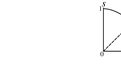
Isotropic copies in which

$$b_{1}=b_{2}=b_{3}=r,\quad c_{1}=c_{2}=c_{3}=s,$$ (135)

that is, the Bloch ellipsoids for ${\cal B}$ and ${\cal C}$ are spheres of radii $r$ and $s$, are obtained by letting

$$\beta_{1}=\beta_{2}=\beta_{3}=\sqrt{(1-\beta_{0}^{2})/3}.$$ (136)

Using (56) and (67), one can show that

$$s={\textstyle{1\over 2}}\left[1-r+\sqrt{(1-r)(1+3r)}\right],$$ (137)

and, by symmetry, $r$ as a function of $s$ is given by precisely the same functional form. The relationship between the two is shown in Fig. 1. Since $r$ is between 0 and 1, the condition (132) for optimal pairs is satisfied. In other words, any point that lies outside the region enclosed by this curve and the two axes is prohibited; this is identical to the no-cloning bound in [12].

FIG. 1.: The relationship between the radii ($s$ and $r$) of the two output Bloch spheres in the case of isotropic copying. Identical copies occur when $r=s=2/3$.

As one might expect, there is a certain “complementarity” between the quality of the copies emerging in the ${\cal B}$ and ${\cal C}$ channels: as $r$ increases, $s$ decreases. Additional insight into the source of this complementarity comes from studying anisotropic situations. Consider, in particular, the extremely anisotropic case in which

$$\beta_{1}=\beta_{2}=0,\quad 0\leq\beta_{3}\leq 1/\sqrt{2};$$ (138)

the upper bound on $\beta_{3}$ ensures that (129) is satisfied. The corresponding $b$ and $c$ for optimal copies are given by

$$b_{1}=b_{2}=1-2\beta_{3}^{2},\quad b_{3}=1,$$ (139)

$$c_{1}=c_{2}=0,\quad c_{3}=2\beta_{3}\sqrt{1-\beta_{3}^{2}}.$$ (140)

Note that as $\beta_{3}$ increases, the quality factor $c_{3}$ for the third principal mode of the ${\cal C}$ copy increases whereas the factor for the same mode of ${\cal B}$ remains perfect, $b_{3}=1$. On the other hand, the quality factors for modes 1 and 2 of ${\cal B}$ decrease as $\beta_{3}$ increases. Thus improving the quality of a particular mode in one channel leads to a decrease in optimal quality of all the “perpendicular” modes of the other channel. In particular, $c_{1}$ and $c_{2}$ are 0 (worthless copies) in this case because of the perfect quality for mode 3 of ${\cal B}$.

VII Quantum Circuit

A complicated unitary transformation can often be decomposed into several simpler transformations and expressed in a pictorial fashion by using a quantum circuit. This is helpful both for understanding the transformation and for implementing it in a systematic way. It is worth noting that any unitary transformation can be produced by a circuit which only uses two-qubit XOR gates along with an appropriate collection of one-qubit gates [17].

From Sec. IV, the optimal copying procedure corresponding to $\mbox{\boldmath$c$}=G(\mbox{\boldmath$b$})$ can always be achieved, for any given $b$, by using a transformation which generates the isometry (62). One example is given by the circuit in Fig. 2(a), where the input state is a tensor product $|\alpha{\rangle}\otimes|\epsilon{\rangle}$, with $|\alpha{\rangle}$ arbitrary, and

$$|\epsilon{\rangle}=\beta_{0}|00{\rangle}+\beta_{1}|01{\rangle}+\beta_{2}|11{\rangle}+\beta_{3}|10{\rangle}.$$ (141)

Since $|\epsilon{\rangle}$ involves only real coefficients, it can be produced by a preparation circuit as shown in [10]. The three horizontal lines represent the three qubits going from left to right, as time increases, through four quantum gates. The order of the qubits from top to bottom is the same as the left-to-right order in (62).

FIG. 2.: (a) Optimal copy circuit. The qubit to be copied enters the circuit as $|\alpha{\rangle}$ on the left, and the copies emerge in $b$ and $c$ on the right. (b) Alternative circuit, see discussion in text.

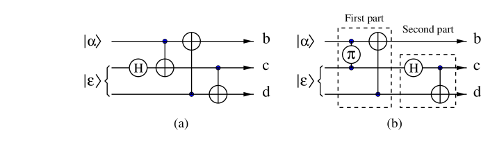
The first gate in Fig. 2(a) produces the Hadamard transform

$$|0{\rangle}\mapsto|\!+\!{\rangle}=(|0{\rangle}+|1{\rangle})/\sqrt{2},$$ (142)

$$|1{\rangle}\mapsto|\!-\!{\rangle}=(|0{\rangle}-|1{\rangle})/\sqrt{2},$$ (143)

on a single qubit. The remaining three gates are XOR gates acting on different pairs of qubits; each corresponds to the transformation

$$|00{\rangle}\mapsto|00{\rangle}, |10{\rangle}\mapsto|11{\rangle},$$ (144)

$$|01{\rangle}\mapsto|01{\rangle}, |11{\rangle}\mapsto|10{\rangle},$$ (145)

in which the left qubit in this formula is the “controlling” and the right qubit the “controlled” qubit. If the controlling qubit is $|0{\rangle}$, the controlled qubit is left unchanged; if the controlling qubit is $|1{\rangle}$, the controlled qubit is flipped from $|0{\rangle}$ to $|1{\rangle}$, or $|1{\rangle}$ to $|0{\rangle}$, which is known as “amplitude-flipping”. In Fig. 2(a) the controlling qubit is indicated by a solid dot, and the corresponding controlled qubit by a plus inside a circle. Thus the controlling qubit is the top, bottom, and middle qubit in the first, second, and third XOR gates.

The transformation produced by the circuit in Fig. 2(a) can be more easily understood if one uses the alternative circuit in Fig. 2(b), which produces exactly the same overall unitary transformation. It employs another gate, indicated by $\pi$ inside a circle connecting two black dots, which produces the transformation

$$|00{\rangle}\mapsto|00{\rangle}, |10{\rangle}\mapsto|10{\rangle},$$ (146)

$$|01{\rangle}\mapsto|01{\rangle}, |11{\rangle}\mapsto-|11{\rangle},$$ (147)

where the phase of $|11{\rangle}$ is multiplied by a factor of $e^{i\pi}=-1$. It flips one qubit between $|\!+\!{\rangle}$ and $|\!-\!{\rangle}$, see (143), if the other qubit is $|1{\rangle}$. This is known as a “phase flip”, in contrast to the “amplitude flip” produced by an XOR gate. Note that in this case either qubit can be regarded as controlling the other.

Both circuits in Fig. 2 carry out the transformation

$$|\alpha{\rangle}\otimes|\epsilon{\rangle}\mapsto\sum_{l}(\sigma_{l}|\alpha{\rangle})\otimes\beta_{l}|\hat{e}_{l}{\rangle}$$ (148)

corresponding to (4) combined with (50), and thus the isometry (62) on the input qubit $|\alpha{\rangle}$. But Fig. 2(b) is a bit easier to interpret. In the first part of the circuit, the lower two qubits control the top qubit: the middle qubit, if it is $|1{\rangle}$, flips the phase, and the bottom qubit, if $|1{\rangle}$, flips the amplitude. Thus this part of the circuit results in

$$|\alpha{\rangle}\otimes|00{\rangle} \mapsto (\sigma_{0}|\alpha{\rangle})\otimes|00{\rangle},$$ (149)

$$|\alpha{\rangle}\otimes|01{\rangle} \mapsto (\sigma_{1}|\alpha{\rangle})\otimes|01{\rangle},$$ (150)

$$|\alpha{\rangle}\otimes|11{\rangle} \mapsto (\sigma_{1}\sigma_{3}|\alpha{\rangle})\otimes|11{\rangle}=(-i\sigma_{2}|\alpha{\rangle})\otimes|11{\rangle},$$ (151)

$$|\alpha{\rangle}\otimes|10{\rangle} \mapsto (\sigma_{3}|\alpha{\rangle})\otimes|10{\rangle},$$ (152)

where $\sigma_{0}$ is the identity, $\sigma_{1}$ flips the amplitude, $\sigma_{3}$ flips the phase, and $\sigma_{1}\sigma_{3}$ flips the phase and then the amplitude. Consequently, a linear superposition of the maps in (152) results in

$$|\alpha{\rangle}\otimes|\epsilon{\rangle}\mapsto\sum_{l}(\sigma_{l}|\alpha{\rangle})\otimes\beta_{l}|\hat{\epsilon}_{l}{\rangle},$$ (153)

where

$$|\hat{\epsilon}_{0}{\rangle}=|00{\rangle},\ |\hat{\epsilon}_{1}{\rangle}=|01{\rangle},\ |\hat{\epsilon}_{2}{\rangle}=-i|11{\rangle},\ |\hat{\epsilon}_{3}{\rangle}=|10{\rangle}.$$ (154)

The second part of the circuit in Fig. 2(b) is a unitary transformation on the lower two qubits which maps each $|\hat{\epsilon}_{l}{\rangle}$ into $|\hat{e}_{l}{\rangle}$, so that the effect of the two parts combined is (148).

This perspective also provides an intuitive meaning for the $\beta_{l}$’s. The action of the superoperator $\hat{V}_{\cal B}$, (18), on the input state

$$\alpha=|\alpha{\rangle}{\langle}\alpha|,$$ (155)

given by

$$\hat{V}_{\cal B}(\alpha)=\sum_{l}\beta^{2}_{l}(\sigma_{l}\alpha\sigma_{l}),$$ (156)

is determined by the first part of the circuit in Fig. 2(b), thus by (153). One can think of (156) as a probabilistic mixture of states obtained by applying the unitary transformation $\sigma_{l}$ with probability $\beta^{2}_{l}$ to the input state $|\alpha{\rangle}$. In other words, $\beta^{2}_{l}$ for $l\neq 0$ is the probability of producing a noise of type $l$ (amplitude or phase flipping, or the combination) in the ${\cal A}{\cal B}$ channel. This defines a Pauli channel, in the notation of [12], and since the ${\cal A}{\cal C}$ channel is of the same type—by the symmetry between (62) and (65)—the corresponding transformation constitutes a Pauli cloning machine as defined in [12]. It is worth mention that even though this Pauli machine is optimal, there exist optimal machines that are not Pauli machines [18].

Finally, note that if $|\epsilon{\rangle}$ is of the tensor product form

$$\left(\sqrt{1-D_{xy}}|0{\rangle}+\sqrt{D_{xy}}|1{\rangle}\right)\otimes\left(\sqrt{1-D_{uv}}|0{\rangle}+\sqrt{D_{uv}}|1{\rangle}\right),$$ (157)

this circuit carries out the optimal eavesdropping in [11] for the case of the BB84 cryptographic system [19]. Here $D_{xy}$ and $D_{uv}$ are the error rates defined in [11]. With $\beta_{1}=\beta_{2}=\beta_{3}=1/\sqrt{12}$ in (141), this circuit carries out Bužek and Hillery’s universal cloning. It is an alternative to the circuit given in [10].

VIII Conclusion

We have shown how to produce two optimal copies of one qubit in the cases in which the quality of the copies can be different, and can depend upon which input mode (orthogonal basis) is employed. The measure of quality of the copies is a distinguishability measure on quantum states, and differs from the fidelity measures used in previous published work. In particular, it uses a geometrical representation in which the output possibilities correspond to ellipsoids in the respective Bloch spheres, with a larger ellipsoid corresponding to higher quality. The copy qualities are “complementary” in the sense that improving the quality of one copy for a particular input mode tends to degrade the quality of the other copy for a different set of input modes. Optimal copies can be achieved by means of a relatively simple quantum circuit.

This represents significant progress towards quantifying the no-cloning theorem of quantum information theory. It is useful in applications to quantum cryptography, in which the “copies” go to the eavesdropper and to the legitimate receiver, and also to quantum decoherence processes, in which one “copy” disappears into the environment. In both of these applications, the copies need not be identical, and their qualities can depend upon the input signal.

There are several respects in which one might hope to extend the results presented here. Producing more than two copies of one qubit with (in general) different qualities for the different copies, and qualities which depend upon the input mode remains to be studied. Extending our results to higher-dimensional Hilbert spaces is a significant challenge, because there seems to be no convenient geometrical representations analogous to a Bloch sphere, nor an analytic form of distinguishability measure for more than two states. Nonetheless, recent progress by Zanardi [20] and Cerf [12] in characterizing anisotropic higher-dimensional copies is encouraging. In addition, one could study optimization using other measures of quality or information [21], including Shannon’s mutual information. Of course it would be extremely interesting to find some general point of view which unifies all the results on quantum copying obtained up to the present.

A Properties of $L(jk;lm)$

The complex conjugate of

$$L(jk;lm)={\textstyle{1\over 2}}\hbox{Tr}[\sigma_{j}\sigma_{l}\sigma_{k}\sigma_{m}]$$ (A1)

is the trace of the $\sigma$’s in reverse order. Invariance of the trace under cyclic permutation then shows that

$$L(kj;lm)=L(jk;ml)=L(lm;jk)=L^{*}(jk;lm).$$ (A2)

That is, interchanging $j$ and $k$, or interchanging $l$ and $m$, or interchanging $jk$ with $lm$ turns $L(jk;lm)$ into its complex conjugate. Suppose that two $4\times 4$ matrices $P$ and $Q$ are related by

$$P_{jk}=\sum_{lm}L(jk;lm)Q_{lm}.$$ (A3)

Then (A2) implies that if $Q$ is real, $P$ is Hermitian, and if $Q$ is Hermitian, $P$ is real.

Explicit values for $L(jk;lm)$ can be obtained in the following way. Suppose that $\zeta$ is the number of the four indices $j$, $k$, $l$, and $m$ that are zero. It is obvious that if $\zeta=4$, $L=1$, and if $\zeta=3$, $L=0$. When $\zeta=2$, $L$ will vanish unless the non-zero indices are equal, in which case

$$L(00;qq)=L(0q;0q)=1.$$ (A4)

If $\zeta=1$, $L$ will vanish unless all the indices are unequal, and by explicit calculation,

$$L(0q;q^{\prime}q^{\prime\prime})=-i,$$ (A5)

using the convention (11). If $\zeta=0$, two of the indices must be equal, and $L$ vanishes unless the other two are also equal to each other. So $L$ is zero except for

$$L(qq;qq)=L(qq^{\prime};qq^{\prime})=1,\quad L(qq;q^{\prime}q^{\prime})=-1,$$ (A6)

with $q^{\prime}\neq q$. The other non-zero elements of $L$ can be obtained from (A4)–(A6) by permuting the indices, using (A2).

Regarded as a map, (A3), $L$ carries certain subspaces of the 16-dimensional space of $4\times 4$ matrices into themselves. Thus if $Q_{jk}=0$ except when $jk$ is equal to 00, 11, 22, and 33, then $P_{jk}$ has the same character, and one can write, see (16),

$$P_{jj}=\sum_{k}\Lambda(j,k)Q_{kk},$$ (A7)

where

$$\Lambda=\left(\matrix{1&\hphantom{-}1&\hphantom{-}1&\hphantom{-}1\cr 1&\hphantom{-}1&-1&-1\cr 1&-1&\hphantom{-}1&-1\cr 1&-1&-1&\hphantom{-}1}\right)$$ (A8)

is its own inverse, apart from a factor of 4:

$$\sum_{k}\Lambda(j,k)\Lambda(k,l)=4\delta_{jl}.$$ (A9)

The other invariant subspaces of $L$ correspond to $jk$ of the form $0q$, $q0$, $q^{\prime}q^{\prime\prime}$, $q^{\prime\prime}q^{\prime}$ in the notation of (11). Hence, thought of as a $16\times 16$ matrix, $L$ is block diagonal with four $4\times 4$ matrices as diagonal blocks. One of these matrices is (A8), and the others can be written down explicitly using (A4) to (A6). In each case the square of the $4\times 4$ matrix is 4 times the identity. Consequently, ${\textstyle{1\over 2}}L$ is its own inverse, or

$$\sum_{lm}L(jk;lm)\,L(lm;rs)=4\delta_{jr}\delta_{ks}.$$ (A10)

B Some Properties of $\hbox{Tr}(|A|)$

The following results hold for a finite-dimensional Hilbert space ${\cal H}$.

Theorem 1. Let $B$ and $C$ be any two positive (Hermitian with non-negative eigenvalues) operators, and let

$$A=B-C.$$ (B1)

Then

$$\hbox{Tr}(|A|)\leq\hbox{Tr}(B)+\hbox{Tr}(C).$$ (B2)

The proof consists in noting that if $\{|\alpha_{j}{\rangle}\}$ is an orthonormal basis which diagonalizes $A$,

$$A=\sum_{j}a_{j}|\alpha_{j}{\rangle}{\langle}\alpha_{j}|,$$ (B3)

then it follows from (B1) that

$$|a_{j}|=|{\langle}\alpha_{j}|A|\alpha_{j}{\rangle}|\leq|{\langle}\alpha_{j}|B|\alpha_{j}{\rangle}|+|{\langle}\alpha_{j}|C|\alpha_{j}{\rangle}|$$ (B4)

$$={\langle}\alpha_{j}|B|\alpha_{j}{\rangle}+{\langle}\alpha_{j}|C|\alpha_{j}{\rangle},$$ (B5)

where the final equality is a consequence of the fact that diagonal matrix elements of a positive operator cannot be negative. Summing (B5) over $j$ yields (B2)

Theorem 2. Let $A$ be a Hermitian operator, and let

$$I=\sum_{k}P_{k}$$ (B6)

be a decomposition of the identity as a sum of mutually orthogonal projectors. Then

$$\sum_{k}\hbox{Tr}(|P_{k}AP_{k}|)\leq\hbox{Tr}(|A|).$$ (B7)

In particular, if $\{|\beta_{k}{\rangle}\}$ is any orthonormal basis of ${\cal H}$,

$$\sum_{k}|{\langle}\beta_{k}|A|\beta_{k}{\rangle}|\leq\hbox{Tr}(|A|),$$ (B8)

since we can set $P_{k}=|\beta_{k}{\rangle}{\langle}\beta_{k}|$ in (B7).

To prove this theorem, write

$$A=A^{\prime}-A^{\prime\prime},$$ (B9)

with $A^{\prime}$ that part of the sum (B3) with $a_{j}\geq 0$, and $-A^{\prime\prime}$ the remainder. Then $A^{\prime}$ and $A^{\prime\prime}$ are positive operators, and $\hbox{Tr}(|A|)$ is the sum of their traces. Define

$$A_{k}=P_{k}AP_{k},\quad A^{\prime}_{k}=P_{k}A^{\prime}P_{k},\quad A^{\prime\prime}_{k}=P_{k}A^{\prime\prime}P_{k},$$ (B10)

and apply theorem 1 to $A_{k}=A^{\prime}_{k}-A^{\prime\prime}_{k}$, to obtain

$$\hbox{Tr}(|A_{k}|)\leq\hbox{Tr}(A^{\prime}_{k})+\hbox{Tr}(A^{\prime\prime}_{k})=\hbox{Tr}(A^{\prime}P_{k})+\hbox{Tr}(A^{\prime\prime}P_{k}),$$ (B11)

where the equality uses $P_{k}^{2}=P_{k}$. Summing (B11) over $k$, see (B6), yields (B7).

Theorem 3. Let $A$ be a Hermitian operator on ${\cal H}={\cal F}\otimes{\cal G}$, and

$$A_{\cal F}=\hbox{Tr}_{\cal G}(A).$$ (B12)

Then

$$\hbox{Tr}_{\cal F}(|A_{\cal F}|)\leq\hbox{Tr}_{\cal H}(|A|).$$ (B13)

The proof consists in writing

$$A_{\cal F}=A^{\prime}_{\cal F}-A^{\prime\prime}_{\cal F},$$ (B14)

where $A^{\prime}_{\cal F}$ and $A^{\prime\prime}_{\cal F}$ are the partial traces over ${\cal G}$ of $A^{\prime}$ and $A^{\prime\prime}$ in (B9). As these are positive operators, theorem 1 tells us that

$$\hbox{Tr}_{\cal F}(|A_{\cal F}|)\leq\hbox{Tr}_{\cal F}(A^{\prime}_{\cal F})+\hbox{Tr}_{\cal F}(A^{\prime\prime}_{\cal F})$$ (B15)

$$=\hbox{Tr}_{\cal H}(A^{\prime})+\hbox{Tr}_{\cal H}(A^{\prime\prime})=\hbox{Tr}_{\cal H}(|A|).$$ (B16)

C Differential of the Optimization Map

The differential relationship (121) can be obtained using the expressions

$$b_{q}=\beta^{2}_{0}+\beta^{2}_{q}-\beta^{2}_{q^{\prime}}-\beta^{2}_{q^{\prime\prime}},$$ (C1)

$$c_{q}=2(\beta_{0}\beta_{q}+\beta_{q^{\prime}}\beta_{q^{\prime\prime}}),$$ (C2)

from (56) and (67), together with, see (55),

$$b_{0}=c_{0}=\beta^{2}_{0}+\beta^{2}_{1}+\beta^{2}_{2}+\beta^{2}_{3}=1.$$ (C3)

Here and in what follows, $q,q^{\prime},$ and $q^{\prime\prime}$ are related using the convention in (11). Let $f$ be some function of $\beta_{0},\beta_{1},\beta_{2},\beta_{3}$ on the manifold (C3). Its differential can be written as

$$df=\sum_{j=0}^{3}(\partial f/\partial\beta_{j})d\beta_{j}=\beta^{-1}_{0}\sum_{q=1}^{3}(\Delta_{q}f)\,d\beta_{q},$$ (C4)

where $d\beta_{0}$ has been eliminated on the right side by setting the differential of (C3) equal to zero, and

$$\Delta_{q}f:=\beta_{0}\partial f/\partial\beta_{q}-\beta_{q}\partial f/\partial\beta_{0}.$$ (C5)

Using (C1), (C2) and (C4), one obtains

$$\beta_{0}\,d\mbox{\boldmath$b$}=-4\mbox{\boldmath$R\,\cdot\,$}d\mbox{\boldmath$\beta$},$$ (C6)

$$\beta_{0}\,d\mbox{\boldmath$c$}=\mbox{\boldmath$S\,\cdot\,$}d\mbox{\boldmath$\beta$},$$ (C7)

with $d\mbox{\boldmath$\beta$}=(d\beta_{1},d\beta_{2},d\beta_{3})$, and the components of the $3\times 3$ matrices $R$ and $S$ are given by:

$$R_{qq}=0,\quad R_{q^{\prime}q}=R_{q^{\prime\prime}q}=\beta_{q},$$ (C8)

$$S_{qq}=2(\beta^{2}_{0}-\beta^{2}_{q}),\quad S_{qq^{\prime}}=S_{q^{\prime}q}=c_{q^{\prime\prime}}.$$ (C9)

The inverse of $R$ is the matrix $Q$, with components

$$Q_{qq}=\beta_{q^{\prime}}\beta_{q^{\prime\prime}},\quad Q_{qq^{\prime}}=Q_{qq^{\prime\prime}}=-\beta_{q^{\prime}}\beta_{q^{\prime\prime}},$$ (C10)

in the sense that

$$\mbox{\boldmath$Q\cdot R$}=\mbox{\boldmath$R\cdot Q$}=-2\beta_{4}\mbox{\boldmath$I$},$$ (C11)

where $\beta_{4}=\beta_{0}\beta_{1}\beta_{2}\beta_{3},$ and $I$ is the identity matrix. Multiplying (C6) by $Q$, solving for $d\mbox{\boldmath$\beta$}$, and inserting the result in (C7) results in (121), with $J$ defined in (123), after some straightforward algebra. A symmetrical argument with $\gamma$ in place of $\beta$ yields (122).

D Miscellaneous results for Sec. VI

That at most one of the $h_{q}$, $q=1,2,3,$ can be negative, follows from the condition

$$0\leq\beta_{q}\leq\beta_{0}\hbox{ for }q=1,2,3,$$ (D1)

which is implied by (120), since if the $\gamma_{j}$ are non-negative, and one writes out the components of $\beta$ in terms of those of $\gamma$, (63), it is obvious that $\beta_{0}$ is at least as large as any of the $\beta_{q}$ for $q>0$. The implications of (D1) can be worked out by assuming, for convenience, the order

$$0\leq\beta_{1}\leq\beta_{2}\leq\beta_{3}\leq\beta_{0}.$$ (D2)

Then it is obvious that

$$\beta_{0}\beta_{3}\geq\beta_{2}\beta_{1},\quad\beta_{0}\beta_{2}\geq\beta_{3}\beta_{1}.$$ (D3)

so that, see (125), $h_{2}$ and $h_{3}$ are non-negative, while $h_{1}$ might be negative. Similar conclusions follow for other orderings.

The proof of the theorem in Sec. VI for the case $\eta=\Lambda\cdot\xi$ can be constructed using the explicit expressions, see (A8),

$$\eta_{0}=\xi_{0}+\xi_{1}+\xi_{2}+\xi_{3},$$ (D4)

$$\eta_{1}=\xi_{0}+\xi_{1}-\xi_{2}-\xi_{3},$$ (D5)

$$\eta_{2}=\xi_{0}-\xi_{1}+\xi_{2}-\xi_{3},$$ (D6)

$$\eta_{3}=\xi_{0}-\xi_{1}-\xi_{2}+\xi_{3}.$$ (D7)

From these it follows that

$$\eta_{q}-\eta_{q^{\prime}}=2(\xi_{q}-\xi_{q^{\prime}}),$$ (D8)

in the notational convention of (11), and this implies (130), which shows that $\eta$ has the same order as $\xi$. Next we show that if $\xi$ belongs to class $P$, that is, its components satisfy the inequalities (129), the same is true of $\eta$. Because the $\xi_{i}$ are non-negative, it follows at once from (D7) that

$$\eta_{q}\leq\eta_{0}.$$ (D9)

Next, a consequence of (D7) is

$$\eta_{0}\eta_{q}-\eta_{q^{\prime}}\eta_{q^{\prime\prime}}=4(\xi_{0}\xi_{q}-\xi_{q^{\prime}}\xi_{q^{\prime\prime}}),$$ (D10)

so that if the components of $\xi$ satisfy the second inequality in (129), so do those of $\eta$. All that remains is to show that

$$\eta_{q}\geq 0.$$ (D11)

If we choose the order of $\xi_{i}$, for convenience, to be

$$0\leq\xi_{1}\leq\xi_{2}\leq\xi_{3}\leq\xi_{0},$$ (D12)

then $\eta_{i}$ has the same order, and it suffices to show that $\eta_{1}\geq 0$. Let us assume $\eta_{1}<0$, which by (D7) implies

$$\xi_{0}-\xi_{2}<\xi_{3}-\xi_{1}.$$ (D13)

By (D12), $\xi_{2}$ is either zero or positive. If $\xi_{2}=0$, then (D12) implies that $\xi_{1}=0$, and (D13) yields $\xi_{0}<\xi_{3}$, in violation of (D12). If $\xi_{2}>0$, then (D12) and (D13) tell us that

$$\xi_{1}(\xi_{0}-\xi_{2})<\xi_{2}(\xi_{3}-\xi_{1}),$$ (D14)

or $\xi_{0}\xi_{1}<\xi_{2}\xi_{3}$, which is to say, the components of $\xi$ do not satisfy the second inequality in (129). This completes the proof.

REFERENCES

• [1] W. K. Wootters and W. H. Zurek, Nature 299, 802 (1982).
• [2] H. Barnum, C. Caves, C. Fuchs, R. Jozsa, and B. Schumacher, Phys. Rev. Lett. 76, 2818 (1996).
• [3] For an introduction to the subject, see C. Bennett, G. Brassard, and A. Ekert, Scientific American, Oct. 1992, p. 50, and R. J. Hughes, D. M. Alde, P. Dyer, G. G. Luther, G. L. Morgan, and M. Schauer, Contemporary Physics 36, 149 (1995).
• [4] V. Bužek and M. Hillery, Phys. Rev. A 54, 1844 (1996).
• [5] D. Bruß, D. P. DiVincenzo, A. Ekert, C. A. Fuchs, C. Macchiavello, and J. A. Smolin, Phys. Rev. A 57, 2368 (1998).
• [6] N. Gisin and S. Massar, Phys. Rev. Lett. 79, 2153 (1997).
• [7] D. Bruß, A. Ekert, and C. Macchiavello, quant-ph/9712019.
• [8] R. F. Werner, quant-ph/9804001.
• [9] V. Bužek and M. Hillery, quant-ph/9801009.
• [10] V. Bužek, S. L. Braunstein, M. Hillery, and D. Bruß, Phys. Rev. A 56, 3446 (1997).
• [11] C. Fuchs, N. Gisin, R. B. Griffiths, C.-S. Niu, and A. Peres, Phys. Rev. A 56, 1163 (1997).
• [12] N. J. Cerf, quant-ph/9805024.
• [13] The same expression derived from a different formalism can be found in I. L. Chuang and M. A. Nielsen, J. of Mod. Opt. 44, 2455 (1997).
• [14] R. A. Horn and C. R. Johnson, Topics in Matrix Analysis (Cambridge University Press, Cambridge, 1991).
• [15] A. Peres, Quantum Theory: Concepts and Methods (Kluwer, Dordrecht, 1993) p. 282.
• [16] C. A. Fuchs, quant-ph/9611010.
• [17] A. Barenco et al., Phys. Rev. A 52, 3457 (1995).
• [18] C.-S. Niu and R. B. Griffiths, in preparation.
• [19] C. Bennett, and G. Brassard, in Proceedings of the IEEE International Conference on Computer, System, and Signal Processing, Bangalore, India (IEEE, New York, 1984), p. 175.
• [20] P. Zanardi, quant-ph/9804011.
• [21] C. A. Fuchs, Ph.D. thesis, University of New Mexico (1995).