FSUJ TPI QO-7/98

May, 1998

Generating and monitoring Schrödinger cats in conditional measurement on a beam splitter
M. Dakna, J. Clausen, L. Knöll, D.–G. Welsch
Friedrich-Schiller-Universität Jena, Theoretisch-Physikalisches Institut

Max-Wien-Platz 1, D-07743 Jena, Germany

Abstract

Preparation of Schrödinger-cat-like states via conditional output measurement on a beam splitter is studied. In the scheme, a mode prepared in a squeezed vacuum is mixed with a mode prepared in a Fock state and photocounting is performed in one of the output channels of the beam splitter. In this way the mode in the other output channel is prepared in a Schrödinger-cat-like state that is either a photon-subtracted or a photon-added Jacobi polynomial squeezed vacuum state, depending upon the difference between the number of photons in the input Fock state and the number of photons in the output Fock state onto which it is projected. Two possible photocounting schemes are considered, and the problem of monitoring cats that are “hidden” in a statistical mixture of states is studied.

1 Introduction

The interference of probability amplitudes is one of the most specific features of quantum theory and it has been discussed since the early days of quantum mechanics. The famous Schrödinger-cat-like states are a typical example. The cat stands for a macroscopic object which may be in a superposition of states corresponding to macroscopically distinguishable beings (living and dead) [1]. However the experimental demonstration of quantum interference effects for macroscopic systems is very difficult due to the irreversible interaction of such a system with its environment [2]. Recent experimental progress has rendered it possible to generate Schrödinger-cat-like states on a mesoscopic scale, as it was successfully demonstrated in neutron interferometry [3] and atom optics in a trap [4].

Despite the large body of work, Schrödinger-cat-like states of optical fields have not been observed so far. Recently a sophisticated method for demonstrating Schrödinger-cat-like states of traveling optical fields by inferring them from noisy data has been proposed [5]. The method is based on the experimental scheme proposed in [6] (see also [7]), and it uses appropriate data processing in order to calculate the intrinsic (undistorted) state from the (distorted) state actually produced and detected.

Recently we have shown that Schrödinger-cat-like states can also be produced by conditional measurement on a beam splitter. In particular, when a mode prepared in a squeezed vacuum is mixed with an ordinary vacuum and a (nonzero) photon-number measurement is performed in one of the output channels of the beam splitter, then the mode in the other output channel is prepared in a Schrödinger-cat-like state [8]. The scheme can be extended to the more general case when the mode prepared in the squeezed vacuum is mixed with a mode prepared in an arbitrary $n$-photon Fock state and the photon-number measurement yields an arbitrary number $m$. The conditional output states are either photon-subtracted ($n$ $\!<$ $\!m$) or photon-added ($n$ $\!>$ $\!m$) Jacobi polynomial squeezed vacuum states, i.e., states that are obtained by ($|n$ $\!-$ $\!m|$ times) repeated application of either the photon destruction operator or the photon creation operator, respectively, to a Jacobi polynomial squeezed vacuum state [9]. It is worth noting that the two classes of states – similarly to the ordinary photon-subtracted ($n$ $\!=$ $\!0$) [8] and photon-added ($m$ $\!=$ $\!0$) [10] squeezed vacuum states – represent Schrödinger-cat-like states.

In this paper we study the properties of these classes of Schrödinger-cat-like states, with special emphasis on the experimental conditions. In fact, due to the extreme fragility of the quantum interferences the attempt to demonstrate them may fail if no rigorous compensation for the detection losses is performed, at least in the conditional measurement. We compare photon chopping [11] (considered in [8]) with single-detector photocounting (considered in [5]) and give an analysis of the corresponding data processing algorithms. Further, the effect of losses in homodyne detection of the states produced is addressed.

This paper is organized as follows. In Sec. 2 we outline the basic scheme for generating photon-subtracted Jacobi polynomial (PSJP) and photon-added Jacobi polynomial (PAJP) squeezed vacuum states and briefly address their properties. In Sec. 3 we compare the two photocounting schemes for conditional measurement and analyse the corresponding algorithms used for processing the experimental data. Finally, in Sec. 4 we give a summary and some concluding remarks.

2 Basis scheme for generating the Schrödinger-cat-like states

The quantum description of the input–output relations of a lossless beam splitter are well known to obey the $\rm SU(2)$ Lie algebra [12]. In the Schrödinger picture, the output-state density operator $\hat{\varrho}_{\rm out}$ can be related to the input-state density operator $\hat{\varrho}_{\rm in}$ as $\hat{\varrho}_{\rm out}\!=\!\hat{V}^{\dagger}\hat{\varrho}_{\rm in}\hat{V}$, where $\hat{V}$ can be given by [12]

$$\hat{V}=e^{-i(\varphi_{T}-\varphi_{R})\hat{L}_{3}}\,e^{-2i\theta\hat{L}_{2}}\,e^{-i(\varphi_{T}+\varphi_{R})\hat{L}_{3}},$$ (1)

with

$$\hat{L}_{2}=\textstyle\frac{1}{2i}(\hat{a}_{1}^{\dagger}\hat{a}_{2}-\hat{a}_{2}^{\dagger}\hat{a}_{1}),\quad\hat{L}_{3}=\textstyle\frac{1}{2}(\hat{a}_{1}^{\dagger}\hat{a}_{1}-\hat{a}_{2}^{\dagger}\hat{a}_{2}).$$ (2)

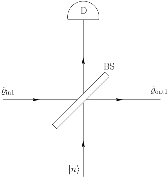
Figure 1: Experimental setup for generating the Schrödinger-cat-like states. A signal mode prepared in a state $\hat{\varrho}_{{\rm in}1}$ $\!=$ $\!\hat{S}(\xi)|0\rangle\langle 0|\hat{S}^{\dagger}(\xi)$ is mixed at the beam splitter BS with another input mode prepared in a Fock state $|n\rangle$, and $m$ photons are recorded by the detector D in one of the output channels of the beam splitter. The quantum state $\hat{\varrho}_{{\rm out}1}$ of the mode in the other output channel is found to be “collapsed” to either a PSJP ($n$ $\!<$ $\!m$) or a PAJP ($n$ $\!>$ $\!m$) squeezed vacuum state.

Let us consider the experimental setup as depicted in Fig. 1. A radiation-field mode prepared in a quantum state $\hat{\varrho}_{{\rm in}1}$ is mixed at a beam splitter with another mode prepared in a Fock state $|n\rangle$, so that the input-state density operator reads as

$$\hat{\varrho}_{\rm in}(n)=\hat{\varrho}_{{\rm in}1}\otimes|n\rangle_{2}\,{}_{2}\langle n|.$$ (3)

The output-state density operator $\hat{\varrho}_{\rm out}$ $\!\equiv$ $\!\hat{\varrho}_{\rm out}(n)$ can then be given by [9]

$$\hat{\varrho}_{\rm out}(n)=\frac{1}{|T|^{2n}}\sum_{l=0}^{\infty}\sum_{m=0}^{\infty}\sum_{k=0}^{n}\sum_{j=0}^{n}\frac{(-1)^{l+m}(R^{*})^{m+j}R^{l+k}}{\sqrt{k!j!m!l!}}\left[{n\!-\!k\!+\!m\choose m}\!{n\!-\!j\!+\!l\choose l}\right]^{\frac{1}{2}}$$ (4)

$$\hskip 12.91663pt\times\left[\!{n\choose k}\!{n\choose j}\right]^{\frac{1}{2}}T^{\hat{n}_{1}}{\hat{a}_{1}}^{m}({\hat{a}_{1}^{\dagger}})^{k}\hat{\varrho}_{{\rm in}1}\hat{a}_{1}^{j}({\hat{a}_{1}^{\dagger}})^{l}(T^{*})^{\hat{n}_{1}}\!\otimes\!|n\!-\!k\!+\!m\rangle_{2}\,{}_{2}\langle n\!-\!j\!+\!l|.$$

From Eq. (4) we see that the output modes are prepared in a highly entangled quantum state in general. When the photon number of the mode in the second output channel is measured and $m$ photons are detected, then the mode in the first output channel is prepared in a quantum state whose density operator $\hat{\varrho}_{{\rm out}1}(n,m)$ reads

$$\hat{\varrho}_{{\rm out}1}(n,m)=\frac{{}_{2}\langle m|\hat{\varrho}_{\rm out}(n)|m\rangle_{2}}{{\rm Tr}_{1}\{_{2}\langle m|\hat{\varrho}_{\rm out}(n)|m\rangle_{2}\}}\,.$$ (5)

The probability of such an event is given by

$$P(n,m)={\rm Tr}_{1}\{_{2}\langle m|\hat{\varrho}_{\rm out}{(n)}|m\rangle_{2}\}$$ (6)

$$=\!\frac{|R|^{-2\nu}n!}{|T|^{2m}m!}\sum_{j=\mu}^{n}\sum_{k=\mu}^{n}(-|R|^{2})^{j\!+\!k}\!{m\choose j\!-\!\nu}\!{m\choose k\!-\!\nu}\!\sum_{p=\delta}^{\infty}\frac{p!|T|^{2p}}{(p\!+\!\nu)!}\!{p\!+\!j\choose j}\!{p\!+\!k\choose k}\langle p|\!\hat{\varrho}_{{\rm in}1}\!|p\rangle,$$

where the abbreviations

$$\nu=n-m,\quad\mu=\max(0,\nu),\quad\delta=\mu-\nu$$ (7)

have been used.

Let us now consider the case when the first input mode is prepared in a squeezed vacuum state $\hat{\varrho}_{{\rm in}1}\!=\!\hat{S}(\xi)|0\rangle\langle 0|\hat{S}^{\dagger}(\xi)$, where

$$\hat{S}(\xi)|0\rangle=\exp\!\left\{-\textstyle\frac{1}{2}\left[\xi(\hat{a}_{1}^{\dagger}){{}^{2}}-\xi^{\ast}\hat{a}_{1}^{2}\right]\right\}|0\rangle=\,(1-|\kappa|^{2})^{\frac{1}{4}}\sum_{p=0}^{\infty}\frac{[(2p)!]^{1/2}}{2^{p}\,p!}\,\kappa^{p}|2p\rangle,$$ (8)

$\xi$ $\!=$ $\!|\xi|e^{i\varphi_{\xi}}$, $\kappa$ $\!=$ $\!-e^{i\varphi_{\xi}}\tanh|\xi|$. Combining Eqs. (4) and (5) and using Eq. (8), we find that the density operator of the output state reads [10]

$$\hat{\varrho}_{{\rm out}1}(n,m)\!=\!|\Psi_{n,m}\rangle\big{\langle}\Psi_{n,m}|,$$ (9)

where

$$|\Psi_{n,m}\rangle\sim\left\{\begin{array}[]{ll}\hat{a}^{|\nu|}\,{\rm P}_{n}^{(|\nu|,\hat{n}-m)}(2|T|^{2}\!-\!1)\hat{S}(\xi^{\prime})|0\rangle&{\rm for}\,n\!<\!m,\\[4.30554pt] (\hat{a}^{\dagger})^{\nu}{\rm P}_{m}^{(\nu,\hat{n}-m)}(2|T|^{2}\!-\!1)\hat{S}(\xi^{\prime})|0\rangle&{\rm for}\,n\!>\!m\end{array}\right.\quad$$ (12)

is a PSJP ($n$ $\!<$ $\!m$) or a PAJP ($n$ $\!>$ $\!m$) squeezed vacuum state [${\rm P}_{l}^{(\alpha,\beta)}(z)$, Jacobi polynomial; $\xi^{\prime}$ $\!=$ $\!|\xi^{\prime}|e^{i(\varphi_{\xi}+2\varphi_{T})}$; $\tanh|\xi^{\prime}|$ $\!=$ $\!|T|^{2}\tanh|\xi|$]. In the photon-number basis $|\Psi_{n,m}\rangle$ reads

$$\hskip 8.61108pt|\Psi_{n,m}\rangle={\cal N}_{n,m}^{-1/2}\sum_{k=\mu}^{n}\frac{(-|R|^{2})^{k}}{(k-\nu)!}{n\choose k}$$ (13)

$$\hskip 30.1388pt\times\,\!\sum_{p=\mu}^{\infty}\frac{(p!)^{-\frac{1}{2}}(p-\nu+k)!}{\Gamma\!\left(\frac{p-\nu}{2}+1\right)}{\textstyle\frac{1}{2}}\!\left\{1\!+\!(-1)^{p-\nu}\right\}\left({\textstyle\frac{1}{2}}\kappa^{\prime}\right)^{(p-\nu)/2}|p\rangle,$$

with $\kappa^{\prime}$ $\!=$ $\!T^{2}\kappa$. From Eq. (13) we easily see that when the difference between the number $n$ of photons in the second input channel of the beam splitter and the number $m$ of photons detected in the second output channel, i.e., the parameter $\nu$ $\!=$ $\!n$ $\!-$ $\!m$, is even (odd), then the mode in the first output channel is prepared in a PSJP or PAJP squeezed vacuum state $|\Psi_{n,m}\rangle$ that contains only Fock states with even (odd) numbers of photons. Similarly to ordinary photon-subtracted and photon-added squeezed vacuum states [8, 9], the PSJP and PAJP squeezed vacuum states are Schrödinger-cat-like states. From Eq. (13) the normalization constant ${\cal N}_{n,m}$ can be calculated to be

$${\cal N}_{n,m}=\sum_{k=\mu}^{n}\frac{(-|R|^{2})^{k}}{(k-\nu)!}{n\choose k}\sum_{j=\mu}^{n}\frac{(-|R|^{2})^{j}}{(j-\nu)!}{n\choose j}\sum_{p=\epsilon}^{\infty}\frac{(2p+k)!(2p+j)!}{(p!)^{2}(2p+\nu)!4^{p}}|\kappa^{\prime}|^{2p},$$ (14)

where $\epsilon$ $\!=$ $\!\max(0,[(1$ $\!-$ $\!\nu)/2])$, $[x]$ being the integer part of $x$. Rewriting Eq. (14) as

$${\cal N}_{n,m}=\frac{1}{|\kappa^{\prime}|^{\nu}}\sum_{k=\mu}^{n}\frac{(-|R|^{2})^{k}}{(k-\nu)!}{n\choose k}\sum_{j=\mu}^{n}\frac{(-|R|^{2})^{j}}{(j-\nu)!}{n\choose j}\frac{\partial^{j-\nu}}{\partial|\kappa^{\prime}|^{j-\nu}}|\kappa^{\prime}|^{j}\sum_{p=0}^{\infty}\frac{(2p+k)!}{(p!)^{2}4^{p}}|\kappa^{\prime}|^{2p}$$ (15)

and using the doubling formula for the gamma function $(2p+k)!$ $\!=$ $\!2^{2p+k}$ $\!\Gamma(p+\frac{k+1}{2})$ $\!\Gamma(p+\frac{k+2}{2})/\sqrt{\pi}$ and the definition of the hypergeometric function, we derive

$${\cal N}_{n,m}\!=\!\frac{1}{|\kappa^{\prime}|^{\nu}}\sum_{k=\mu}^{n}\!\frac{k!(-|R|^{2})^{k}}{(k\!-\!\nu)!}{n\choose k}\!\sum_{j=\mu}^{n}\!\frac{(-|R|^{2})^{j}}{(j\!-\!\nu)!}{n\choose j}\!\frac{\partial^{j-\nu}}{\partial|\kappa^{\prime}|^{j\!-\!\nu}}|\kappa^{\prime}|^{j}{\rm F}(\textstyle{\frac{k+1}{2},\frac{k+2}{2}},1;|\kappa^{\prime}|^{2}).$$ (16)

Note that the hypergeometric function in Eq. (16) is proportional to a Legendre polynomial, ${\rm F}(\frac{k+1}{2},\frac{k+1}{2},1,|\kappa^{\prime}|^{2})$ $\!=$ $\!(1\!-\!|\kappa^{\prime}|^{2})^{-(k+1)/2}$ $\!\rm{P}_{k}[(1\!-\!|\kappa^{\prime}|)^{-1/2}]$, so that Eq. (16) may be given by

$${\cal N}_{n,m}=\sum_{k=\mu}^{n}\frac{(-|R|^{2})^{k}}{(k-\nu)!}{n\choose k}\sum_{j=\mu}^{n}\frac{j!(-|R|^{2})^{j}}{(j-\nu)!}{n\choose j}\sum_{l=\delta}^{j-\nu}{j-\nu\choose l}\frac{(k+2l^{\prime})!|\kappa^{\prime}|^{2l^{\prime}}}{2^{2l^{\prime}-l}(l+\nu)!l^{\prime}!}$$ (17)

$$\times\frac{\Gamma(\textstyle{l^{\prime}+1/2})}{\Gamma(\textstyle{2l^{\prime}-l+1/2})}\,_{3}{\rm F}_{2}(\textstyle{l^{\prime}+\frac{k+1}{2},l^{\prime}+\frac{k+2}{2},l^{\prime}+\frac{1}{2},l^{\prime}+1,2l^{\prime}-l+1/2};|\kappa^{\prime}|^{2}),$$

where $l^{\prime}\!=\![(l+1)/2]$. The hypergeometric function ${}_{3}{\rm F}_{2}(a_{1},a_{2},a_{3},b_{1},b_{2};z)$ in Eq. (17) can be calculated using standard routines. In particular, it may be expressed in terms of the more familiar hypergeometric function ${}_{2}{\rm F}_{1}(a_{1},a_{2},b_{1};z)$ $\!\equiv$ $\!{\rm F}(a_{1},a_{2},b_{1};z)$. The probability $P(n,m)$ of producing the state $|\Psi_{n,m}\rangle$ is found from Eq. (6) to be

$$P(n,m)=\frac{m!}{n!}\frac{(1-|\kappa|^{2})^{1/2}}{|R|^{2\nu}|T|^{2m}}{\cal N}_{n,m}.$$ (18)

To illustrate the properties of $|\Psi_{n,m}\rangle$, in Fig. 2 the quadrature-component distributions and the Wigner function of a PSJP squeezed vacuum state for $n$ $\!=$ $\!1$ and $m$ $\!=$ $\!4$ are plotted [$P(n,m)$ $\!=$ $\!3.37\%$]. From an inspection of the figure, the state is seen to exhibit all the typical features of a Schrödinger-cat-like state. In particular, a more detailed analysis reveals that the Wigner function is a superposition of two quasi-Gaussian lobes with an interference structure between them. Since the corresponding formulas are rather lengthy, here we do without them and only give an explicit expression of the Husimi function, $Q(x,y)$ $\!=$ $\!|\langle\alpha|\Psi_{n,m}\rangle|^{2}/(2\pi)$, $\alpha$ $\!=$ $\!2^{-1/2}(x+iy)$, which takes the form

$$Q_{n}(x,y|m)=\frac{|R|^{4\nu}|T|^{4m}}{2\pi{\cal N}_{n,m}}|\alpha|^{2\nu}e^{-|\alpha|^{2}}\exp\!\left\{{\textstyle\frac{1}{2}}({\kappa^{\prime}}^{\ast}\alpha^{2}+\kappa^{\prime}{\alpha^{\ast}}^{2})\right\}$$ (19)

$$\hskip 43.05542pt\times\,\Bigg{|}\sum_{k=\delta}^{m}{n\choose k\!+\!\nu}\left(\frac{|R|^{2}}{|T|^{2}}\sqrt{{\textstyle\frac{1}{2}}\kappa^{\prime}{{}^{\ast}}\alpha}\right)^{k}{\rm H}_{k}\!\left(\sqrt{{\textstyle\frac{1}{2}}\kappa^{\prime}{{}^{\ast}}\alpha}\right)\Bigg{|}^{2}.$$

3 $N$-fold photon chopping versus single-detector photocounting

Among the practical problems that may be encountered in an experimental generation of the Schrödinger-cat-like states, the losses associated with nonperfect photon-number measurement may be of primordial importance. For the sake of transparency let us restrict attention to the simplest situation and assume that an ordinary vacuum enters the second input of the beam splitter [8]. In this case Eq. (13) reduces to

$$|\Psi_{0,m}\rangle\equiv|\Psi_{m}\rangle={\cal N}_{m}^{-1/2}\sum_{n=0}^{\infty}\frac{{\rm H}_{m+n}(0)}{\sqrt{n!}}\left(-{\textstyle\frac{1}{2}}\kappa^{\prime}\right)^{(n+m)/2}|n\rangle,$$ (20)

with

$${\cal N}_{m}=\frac{i^{m}m!}{|\kappa^{\prime}|}\left(\frac{|\kappa^{\prime}|^{2}}{1-|\kappa^{\prime}|^{2}}\right)^{(m+1)/2}{\rm P}_{m}\!\left(-i\sqrt{\frac{|\kappa^{\prime}|^{2}}{1-|\kappa^{\prime}|^{2}}}\right)$$ (21)

[$P_{n}(z)$, Legendre Polynomial], and the probability $P(0,m)$ $\!\equiv$ $\!P(m)$ of producing the state $|\Psi_{m}\rangle$ can be given by

$$P(m)=\frac{i^{m}|R|^{2m}|\kappa^{\prime}|^{m}\sqrt{1-|\kappa|^{2}}}{|T|^{2m}(1-|\kappa^{\prime}|^{2})^{(m+1)/2}}\,{\rm P}_{m}\!\left(-i\sqrt{\frac{|\kappa^{\prime}|^{2}}{1-|\kappa^{\prime}|^{2}}}\right),$$ (22)

which is nothing but the probability of detecting $m$ photons in the readout mode.

At present two types of highly efficient photodetectors are available: the linear-response photodiodes suitable for measuring strong signals without single-photon resolution and the avalanche photodiodes that may achieve single-event discrimination but are then saturated. It has therefore been suggested to spread a field whose photon-number statistics is desired to be detected over an array of such highly efficient avalanche photodiodes, on using passive optical multiports. Following [11], we refer to this method as photon-chopping and to the photodiodes as type $I$ detectors. For a $2N_{I}$-port apparatus the probability of recording $k$ coincident events when $m$ photons are present is given by

$$\tilde{P}_{N_{I}}(k|m)=\frac{1}{N_{I}^{m}}{N_{I}\choose k}\sum_{l=0}^{k}(-1)^{l}{k\choose l}(k-l)^{m}$$ (23)

for $k\leq m$, and $\tilde{P}_{N_{I}}(k|m)\!=\!0$ for $k\!>\!m$. Note that $\tilde{P}_{N_{I}}(k|m)\!\to\!\delta_{k,m}$ for $N_{I}\!\to\!\infty$. In Eq. (23) perfect detection is assumed. The effect of nonperfect detection may be modelled by placing an absorber in front of the signal before it enters the $2N_{I}$ port. This corresponds to a random process such that photons are excluded from detection with probability $1\!-\!\eta_{I}$, $\eta_{I}$ being the efficiency of the photodiodes (Note that typically $\eta_{I}$ $\!=$ $\!0.8\ldots 0.94$). The probability of recording $k$ coincident events then modifies to

$$\tilde{P}_{N_{I},\eta_{I}}(k|m)=\sum_{l}\tilde{P}_{N_{I}}(k|l)\,M_{l,m}(\eta_{I}),$$ (24)

where the matrix $M_{l,m}(\eta_{I})$ is given by

$${M}_{l,m}(\eta_{I})={m\choose l}\eta_{I}^{l}(1-\eta_{I})^{m-l}$$ (25)

for $l\!\leq\!m$, and ${M}_{l,m}(\eta_{I})\!=\!0$ for $l\!>\!m$. Since detection of $k$ coincident events can result from various numbers $m$ of photons, the conditional measurement yields a statistical mixture

$$\hat{\varrho}_{I}(k)=\sum_{m}P_{N_{I},\eta_{I}}(m|k)\,|\Psi_{m}\rangle\langle\Psi_{m}|$$ (26)

rather than a pure state $|\Psi_{m}\rangle$. In Eq. (26), $P_{N_{I},\eta_{I}}(m|k)$ is the probability of $m$ photons being present under the condition that $k$ coincident events are recorded. The conditional probability $P_{N_{I},\eta_{I}}(m|k)$ can be obtained using the Bayes rule,

$$P_{N_{I},\eta_{I}}(m|k)=\frac{1}{\tilde{P}_{N_{I},\eta_{I}}(k)}\tilde{P}_{N_{I},\eta_{I}}(k|m)\,P(m).$$ (27)

Here, $P(m)$ is the prior probability (22) of $m$ photons being present, and accordingly, $\tilde{P}_{N_{I},\eta_{I}}(k)$ is the prior probability of recording $k$ coincident events,

$$\tilde{P}_{N_{I},\eta_{I}}(k)=\sum_{m}\tilde{P}_{N_{I},\eta_{I}}(k|m)\ P(m).$$ (28)

Let us now consider a so-called type $II$ detector that is able to discriminate between zero, one and a few more photons, but with low detection efficiency ($\eta_{II}$ $\!\sim$ $\!0.3$). Using such a (single) detector for measuring the photon number yields

$$\hat{\varrho}_{II}(k)=\sum_{m}P_{\eta_{II}}(m|k)\,|\Psi_{m}\rangle\langle\Psi_{m}|,$$ (29)

where, according to the Bayes rule, the conditional probability $P_{\eta_{II}}(m|k)$ is now given by

$$P_{\eta_{II}}(m|k)=\frac{1}{P_{\eta_{II}}(k)}M_{k,m}(\eta_{II})P(m),$$ (30)

with

$$P_{\eta_{II}}(k)=\sum_{m}M_{k,m}(\eta_{II})P(m).$$ (31)

In order to compare the conditional output states that are produced in the two schemes of photon-number measurement, we have calculated the (dimensionless) Shannon entropy

$$S_{I(II)}=-\sum_{m}P_{I(II)}(m|k)\,\ln P_{I(II)}(m|k)$$ (32)

of the statistical mixtures of states,

$$\hat{\varrho}_{I(II)}(k)=\sum_{m}P_{I(II)}(m|k)\,|\Psi_{m}\rangle\langle\Psi_{m}|,$$ (33)

as given by Eqs. (26) and (29). The Shannon entropy is a measure of the spread of the distribution $P_{I(II)}(m|k)$, i.e., it is a measure of the deviation of $\hat{\varrho}_{I(II)}$ from a pure state. Note that for a pure state $S_{I(II)}$ $\!=$ $\!0$ is valid. From Fig. 3 we see that $S_{I}$ can always be reduced below $S_{II}$ when the number of type $I$ detectors in the photon chopping scheme is sufficiently increased. Hence photon chopping (with type $I$ detectors) may be much more suitable for preserving the quantum interference features in the conditional output state than the use of a single type $II$ detector. Photon chopping yields a mixed state that is less spread and “more pure” than the state obtained by using a single type $II$ detector for photon-number measurement. Clearly, when in the photon chopping scheme type $II$ detectors are used in order to record coincident events, then this scheme is less suitable for photon counting than a single type $II$ detector. For $\eta_{I}$ $\!=$ $\!\eta_{II}$ the two schemes yield equal conditional output states only in the limit when $N_{I}$ $\!\to$ $\!\infty$. For finite $N_{I}$ there is always a nonvanishing probability that the number of recorded coincident events is smaller than the number of photons, Eq. (23). In particular with regard to pure-state generation we have

$$\lim_{N_{I}\to\infty}\lim_{\eta_{I}\to 1}S_{I}=0,\quad\lim_{\eta_{II}\to 1}S_{II}=0.$$ (34)

The conditional output states (26) and (29) can be determined using balanced homodyne detection and measuring the quadrature-component distributions

$$p_{I(II)}(x,\varphi|k)=\sum_{m}P_{I(II)}(m|k)\,p(x,\varphi|m),$$ (35)

where [8]

$$p(x,\varphi|m)=|\langle x,\varphi|\Psi_{m}\rangle|^{2}=\frac{|\kappa^{\prime}|^{m}}{2^{m}{\cal N}_{m}\sqrt{\pi\Delta^{m+1}}}\exp\!\left(-\frac{1-|\kappa^{\prime}|^{2}}{\Delta}\,x^{2}\right)\left|{\rm H}_{m}\!\left(Kx\right)\right|^{2},$$ (36)

with $\Delta$ $\!=$ $\!1$ $\!+$ $\!|\kappa^{\prime}|^{2}$ $\!+$ $\!2|\kappa^{\prime}|\cos(2\varphi-\varphi_{\kappa^{\prime}})$ and $K$ $\!=$ $\!\sqrt{(-{\kappa^{\prime}}^{\ast}e^{i2\varphi}-|\kappa^{\prime}|^{2})/\Delta}\,$. In Fig. 4 we report the results of simulated measurements. In the case of a single type $II$ detector, Fig. 4(a), the quantum interferences are totally smeared and non-observable. Although somewhat smeared, the quantum interferences are observable in a photon-chopping scheme with type $I$ detectors, Fig. 4(b). The result obviously reflects the above mentioned fact that the conditional output state $\hat{\varrho}_{II}$, Eq. (29), is “more mixed” than the state $\hat{\varrho}_{I}$, Eq. (26), in general.

The reconstruction of the states $|\Psi_{m}\rangle$ from the mixed state $\hat{\varrho}_{II}(k)$, Eq. (29), can be achieved using the inverse Bernoulli transform [5],

$$|\Psi_{m}\rangle\langle\Psi_{m}|=\frac{1}{P(m)\eta_{II}^{m}}\sum_{k=m}^{\infty}{k\choose m}(1\!-\!\eta_{II}^{-1})^{k-m}P_{\eta_{II}}(j)\hat{\varrho}_{II}(k).$$ (37)

Similarly, inverting Eq. (26), we obtain ($N_{I}$ $\!\to$ $\!\infty$)

$$|\Psi_{m}\rangle\langle\Psi_{m}|=\frac{1}{P(m)\eta_{I}^{m}}\!\sum_{j=m}^{\infty}\!{j\choose m}(1\!-\!\eta_{I}^{-1})^{j-m}\left[\sum_{k=j}^{\infty}(\tilde{P}_{N_{I}})^{-1}_{j,k}\tilde{P}_{N_{I},\eta_{I}}(k)\hat{\varrho}_{I}(k)\right],$$ (38)

where $(\tilde{P}_{N_{I}})^{-1}_{m,k}$ is the inverse of the matrix $(\tilde{P}_{N_{I}})_{k,m}$ $\equiv$ $\!\tilde{P}_{N_{I},\eta_{I}}(k|m)$, and the following recursion relation is valid [11]:

$$(\tilde{P}_{N_{I}})^{-1}_{n,n+k}=\frac{-1}{(\tilde{P}_{N_{I}})_{n+k,n+k}}\sum_{j=0}^{k-1}(\tilde{P}_{N_{I}})^{-1}_{n,n+j}(\tilde{P}_{N_{I}})_{n+j,n+k},\quad k=0,1,2\cdots\,.$$ (39)

Note that Eq. (38) reproduces the exact components $|\Psi_{m}\rangle\langle\Psi_{m}|$ only for $N_{I}\!\to\!\infty$.

Applying Eq. (37) and Eq. (38) (for finite $N_{I}$), the states $|\Psi_{m}\rangle$ can be reconstructed from the homodyne data of the measured mixed states. Examples of reconstructed quadrature-component distributions are shown in Fig. 5. From the figure we see that processing the homodyne data according to Eqs. (37) and (38) allows us to restore the quantum interferences in the quadrature-component distributions of the component states of the produced statistical mixtures of states. It should be noted that with increasing number of measurements the Bernoulli inversion in Eq. (37) yields the almost perfect interference structure [Fig. 5(a)]. In order to realize (for the same number of measurements) a comparable accuracy on the basis of Eq. (38), a sufficiently large number $N_{I}$ of channels (type $I$detectors) in the photon-chopping scheme must be used [$N_{I}$ $\!=$ $\!50$ in place of $N_{I}$ $\!=$ $\!20$ used in Fig. 5(b)]. This is obviously due to the fact that in the photon-chopping scheme the probability that a photon impinges on an already saturated photodiode approaches zero only for $N_{I}$ $\!\to$ $\!\infty$. On the other hand, photon chopping already yields reasonable results for small amounts of data, even when the number of channels is reduced [Fig. 5(d)]. From Fig. 5(c) it is seen that the error in the single-(type-$II$-)detector scheme drastically increases with decreasing number of measurements. This result tells us that photon-chopping may be more powerful than a single-detector scheme when the produced state tends to a macroscopical one and the amount of data needed becomes great.

Finally, let us mention that with respect to the probability of producing particularly macroscopic Schrödinger-cat-like states the chopping scheme may be more suitable than the single-detector scheme. In fact, from Fig. 6 we see that the probability of recording $k$ $\!>$ $\!0$ clicks is always higher for the photon-chopping method as for the single-detector scheme. This effect can be made a bit more pronounced choosing larger $N_{I}$.

Let us briefly comment on the use of a nonperfect homodyne detector for measuring the quadrature-component distributions (35). Since in a realistic homodyne experiment the quadrature components cannot be measured exactly, we may assume that instead of $p_{I(II)}(x,\varphi|k)$ smeared distributions

$$p_{I(II)}(x,\varphi;\eta|k)=\sum_{m}P_{I(II)}(m|k)\,p(x,\varphi;\eta|m)$$ (40)

are measured, where

$$p(x,\varphi;\eta|m)=\int_{-\infty}^{\infty}dy\,f(x-y;\eta)\,p(y,\varphi|m),$$ (41)

$f(x;\eta)$ being some positive single-peaked function of $x$, such as a Gaussian,

$$f(x;\eta)=\frac{1}{\sqrt{2\pi\sigma^{2}}}\exp\!\left(-\frac{x^{2}}{2\sigma^{2}}\right),\quad\sigma=\frac{1-\eta}{2\eta}$$ (42)

($\eta$, quantum efficiency of the homodyne detector, with $\eta$ $\!\leq$ $\!1$). Combining Eqs. (41), (36), and (42) and performing the $y$-integration yields

$$p(x,\varphi;\eta|m)=\frac{|\kappa^{\prime}|^{m}|K|^{2m}}{p^{m+1/2}{\cal N}_{m}\sqrt{2\pi\Delta^{m+1}\sigma^{2}}}\exp\!\left(-\frac{1-(2p\sigma^{2})^{-1}}{2\sigma^{2}}\,x^{2}\right)$$ (43)

$$\hskip 43.05542pt\times\sum_{k=0}^{m}{m\choose k}^{2}(m-k)!\left(\frac{|p-K^{2}|}{2|K|^{2}}\right)^{k}\left|{\rm H}_{k}\!\left(\frac{Kx}{2\sigma^{2}\sqrt{p^{2}-pK^{2}}}\right)\right|^{2}\!,$$

$p$ $\!=$ $\!(1$ $\!-$ $\!|\kappa^{\prime}|^{2})/\Delta$ $\!+$ $\!1/(2\sigma)$. It can be readily seen from Eqs. (41) – (43) that $p(x,\varphi;\eta|m)$ $\!\to$ $\!p(x,\varphi|m)$ for $\eta$ $\!\to$ $\!1$. The notorious fragility of the interference structure may be directly seen by comparing the quadrature-component distributions (36) and (43). For example, for $m$ $\!=$ $\!3$ (an a mean number of photons $\langle\hat{n}\rangle$ $\!=$ $\!15$) the interference structure is completely smeared out if $\eta$ $\!<$ $\!0.94$ (Fig. 7).

It is well known that for compensating the losses of the homodyne detector one can make a detour via the density matrix in the Fock representation. The density-matrix elements are reconstructed from the noisy quadrature-component distributions using loss-compensating kernels,

$$\hat{\varrho}_{n,n^{\prime}}(m)=\langle n|\Psi_{m}\rangle\langle\Psi_{m}|n^{\prime}\rangle=\int_{2\pi}\,d\varphi\int_{-\infty}^{\infty}\,d\,x\,p(x,\varphi;\eta|m)K_{n,n^{\prime}}(x,\varphi;\eta),$$ (44)

$K_{n,n^{\prime}}(x,\varphi;\eta)$ being given in [13] (note that such a compensation is possible only for $\eta$ $\!>$ $\!0.5$). Alternatively one can first reconstruct the density-matrix elements in the Fock basis using the kernel functions for perfect detection and then apply an inverse Bernoulli transform to reconstruct the true density-matrix elements [14].

4 Summary

We have shown that quantum-state preparation via conditional output measurement on a beam splitter can be advantageously used for preparation of a great variety of Schrödinger-cat-like states. When a mode prepared in a squeezed vacuum and a mode prepared in an arbitrary Fock state are superimposed by a beam splitter and an arbitrarily chosen number of photons is recorded in one of the output channels of the beam splitter, then the mode in the other output channel is prepared in either a photon-subtracted or a photon-added Jacobi polynomial squeezed vacuum state, the latter being obtained by applying an operator-valued Jacobi polynomial to a squeezed vacuum state. All the PSJP and PAJP states represent examples of Schrödinger-cat-like states, provided that the sum of the number of incident photons and the number of detected photons is nonzero.

In order to project onto Fock states, we have studied two methods of direct photon counting which may be realized with currently available techniques: single-detector photon counting and $N$-fold photon chopping. Both methods produce statistical mixtures of Schrödinger-cat-like states rather than pure states in general, because of nonperfect detection. We found that photon chopping offers the possibility of direct observation of the quantum interferences. Moreover this method can be advantageously used to reduce the amount of data needed for reconstructing the Schrödinger-cat-like states in the produced mixed state, which can be measured by balanced homodyning. When the number of recorded data is suitably large, then the use of a single (low-efficiency) detector may be more advantageous. In this case the pure-state components of the statistical mixture of states can simply be calculated from the measured data using the inverse Bernoulli transform. To realize the same accuracy in photon chopping, the number of channels and detectors must be relatively high.

Acknowledgements This work was supported by the Deutsche Forschungsgemeinschaft.

Figure 2: Quadrature distribution (a) and the Wigner function (b) of a PSJP squeezed vacuum $|\Psi_{n,m}\rangle$ [$n\!=\!1$ and $m\!=\!4$] for $\kappa^{\prime}\!=-\!0.81$ [$|T|^{2}\!=\!0.9$, $|\kappa|\!=\!0.9$].

Figure 3: The Shannon entropies $S_{I}$ and $S_{II}$ of the mixed states (26) and (29), respectively. In (a) it is assumed that $k$ $\!=$ $\!3$ events are recorded and the quantum efficiencies are $\eta_{I}$ $\!=$ $\!0.85$ and $\eta_{II}$ $\!=$ $\!0.3$. In (b) the parameters are $k$ $\!=$ $\!5$ and $\eta_{I}\!=\!0.5$ and $\eta_{II}\!=\!0.3$. The calculations are performed for $\kappa^{\prime}$ $\!=$ $\!-0.7$ ($|T|^{2}$ $\!=$ $\!0.9$, $|\kappa|$ $\!=$ $\!0.77$).

Figure 4: The quadrature-component distributions $p_{II}(x,\varphi|k)$ (a) and $p_{I}(x,\varphi|k)$ (b), respectively, of the mixed states (29) ($\eta_{II}$ $\!=$ $\!0.3$) and (26) ($N_{I}$ $\!=$ $\!20$, $\eta_{I}$ $\!=$ $\!0.9$) are shown for $\varphi$ $\!=$ $\!0$ and $k$ $\!=$ $\!3$. The theoretical distributions (36) (solid lines) are compared with the histograms obtained from computer-simulations of $10^{6}$ measurements. The calculations are performed for $\kappa^{\prime}$ $\!=$ $\!-0.81$ ($|T|^{2}$ $\!=$ $\!0.9$, $|\kappa|$ $\!=$ $\!0.9$).

Figure 5: The quadrature-component distributions $p(x,\varphi|m)$ of $|\Psi_{m}\rangle$ reconstructed from the homodyne data, (a,c) according to Eq. (37) ($\eta_{II}$ $\!=$ $\!0.3$) and (b,d) according to Eq. (38) ($N_{I}$ $\!=$ $\!20$, $\eta_{I}$ $\!=$ $\!0.9$), are shown for $\varphi$ $\!=$ $\!0$ and $m$ $\!=$ $\!3$. The theoretical distribution (36) (solid line) is compared with the distributions reconstructed from (a,b) $5\cdot 10^{5}$ measurement, (c) $10^{4}$ measurements, and (d) $10^{3}$ measurements. The calculations are performed for $\kappa^{\prime}$ $\!=$ $\!-0.81$ ($|T|^{2}$ $\!=$ $\!0.9$, $|\kappa|$ $\!=$ $\!0.9$).

Figure 6: The prior probabilities (28) (solid bars) and (31) (dashed bars) for recording $k$ clicks in the photon-chopping scheme ($\eta_{I}$ $\!=$ $\!0.9$, $N_{I}$ $\!=$ $\!20$) and the single-detector scheme ($\eta_{II}$ $\!=$ $\!0.3$), respectively, are shown. The calculations are performed for $\kappa^{\prime}$ $\!=$ $\!-0.81$ ($|T|^{2}$ $\!=$ $\!0.9$, $|\kappa|$ $\!=$ $\!0.9$). Note that for $k\!=\!3$ the type $II$ detector only gives $12\%$ of the probability obtained by photon chopping.

Figure 7: The theoretical quadrature-component distribution (36) at the phase $\varphi$ $\!=$ $\!0$ (solid line) is compared with the quadrature-component distribution (43) obtained in nonperfect homodyne detection for $\eta$ $\!=$ $\!0.98$ (dashed line) and $\eta$ $\!=$ $\!0.94$ (dotted line). The values of the other parameters are as in Fig. 3 The calculations are performed for $\kappa^{\prime}$ $\!=$ $\!-0.81$ ($|T|^{2}$ $\!=$ $\!0.9$, $|\kappa|$ $\!=$ $\!0.9$).

References

• [1] E. Schrödinger, Naturwissenschaften 23, (1935) 807.
• [2] W.H. Zurek, Phys. Today 44, (1991) 36; 46, (1993) 81.
• [3] D.L. Jacobson, S.A. Werner, H. Rauch. Phys. Rev. A 49, (1994) 3196.
• [4] C. Monroe, D.M. Meekhof, B.E. King, D.J. Wineland, Science 272, (1996) 1131.
• [5] G.M. D’Ariano, C. Machiavello, L. Maccone, [Los Alamos e-print archive quant-ph/9804021 (1998)].
• [6] S. Song, C. M. Caves, B. Yurke, Phys. Rev. A 41, (1990) 5261.
• [7] B. Yurke, W. Schleich and D. F. Walls, Phys. Rev. A 42, (1990) 1703.
• [8] M. Dakna, T. Anhut, T. Opatrný, L. Knöll, D.–G. Welsch, Phys. Rev. A 55, (1997) 3184.
• [9] M. Dakna, L. Knöll, D.–G. Welsch, to appear in Europ. Phys. J. D [Los Alamos e-print archive quant-ph/9803077 (1998)].
• [10] M. Dakna, L. Knöll, D.–G. Welsch Opt. Commun. 145, (1998) 309.
• [11] H. Paul, P. Törmä, T. Kiss, I. Jex, Phys. Rev. Lett. 77, (1996) 2446.
• [12] R.A. Campos, B.E.A. Saleh, M.C. Teich, Phys. Rev. A 40, (1989) 1371,
• [13] G. M. D’Ariano, U. Leonhardt, H. Paul, Phys. Rev. A 52, (1995) R1801.
• [14] T. Kiss, U. Herzog, U. Leonhardt, Phys. Rev. A 52, (1995) 2433.
Refer to caption