Hydrodynamical quantum state reconstruction

Abstract

The density matrix of a nonrelativistic wave-packet in an arbitrary, one-dimensional and time-dependent potential can be reconstructed by measuring hydrodynamical moments of the Wigner distribution. An $n$-th order Taylor polynomial in the off-diagonal variable is obtained by measuring the probability distribution at $n+1$ discrete time values.

This Letter presents a new and general method for reconstructing the density matrix of a massive particle in an arbitrary, one-dimensional and time-dependent potential. Such a general method may seem called for, e.g., in the reconstruction of the quantum state of particles in anharmonic, time-dependent Paul traps. The method is based upon measuring the position probability distribution for a discrete number of time values in a short time interval. Surprisingly, the method follows almost immediately from known results.

The diagonal of the density matrix can be retrieved by observing a single probability distribution. The state reconstruction problem essentially consists in obtaining the offdiagonal elements. Decoherence and the approach to the classical regime is characterized by a vanishing of the offdiagonal elements [1]. The method presented here is constructed so that the density matrix is retrieved for increasing values of the off-diagonal variable by increasing the number of discrete time values for which the probability density is observed.

It was shown by Madelung [2] that quantum mechanics can be reformulated in a form resembling a hydrodynamical description. He reformulated the Schrödinger equation as two coupled and nonlinear equations for the “hydrodynamical” moments of probability density and probability current density. Whereas these two moments can describe a pure state [3], the situation is more complicated for mixed states.

A somewhat analogous situation is found in classical statistical mechanics. Hilbert [4] demonstrated that the phase space distribution for a system in local thermal equilibrium can be expressed as a functional of the density, the current density and the kinetic energy density. These are the three lowest order velocity moments of the phase space distribution. Thus, in thermal equilibrium the phase space distribution is equivalent to it’s three lowest order moments. This situation has sometimes been called the Hilbert paradox [5]. In general, though, an infinite set of velocity moments is equivalent to the full phase space distribution. These moments are coupled through an infinite set of differential equations. In the case of thermal equilibrium this set is truncated, and a finite and closed set of equations is obtained.

The similarity between quantum mechanics and statistical mechanics goes beyond the observation made by Madelung, which is restricted to pure states. Wigner [6] showed that quantum mechanics can be reformulated in terms of a quasi phase space distribution. This distribution, which is the Fourier transform of the density matrix, shares most of the properties of a classical phase space distribution. One important exception is that it may take on negative values. It can be shown [7] that the probability density and the probability current density are the first two velocity moments of the Wigner distribution. This is in complete analogy with classical statistical mechanics. An infinite hierarchy of velocity moments can be derived from the Wigner distribution, and they are interconnected through an infinite set of coupled equations, much like in classical statistical mechanics.

However, quantum mechanics can offer more. It has been shown [8, 9, 10, 11] that when the density matrix in position representation is expanded as a Taylor series in the offdiagonal variable, the coefficients of this expansion are velocity moments of the Wigner distribution. This in fact solves the moment problem both for classical statistical mechanics and for quantum mechanics. With “the moment problem” we here mean the problem of expressing a distribution in terms of it’s moments. This is a classical problem in statistics, and it was first raised in the context of quantum mechanics by Moyal [8]. It was further explored in Ref. [12]. Recently, the density matrix was expressed in terms of normally ordered moments [13]. It has also been shown [14] that the normally ordered moments can be calculated from the measured quadrature distribution. Since convergent expansions may be found [15], this gives a method for reconstructing the state of a radiation field or a particle in a harmonic oscillator potential.

The possibility of measuring quantum states has attracted a lot of attention in recent years. In particular, the method of homodyne tomography [16, 17] has contributed to this interest. It has been used to reconstruct the quantum state of radiation fields [18] as well as material particles propagating in free space [19]. In homodyne tomography the state is retrieved from a parameterized probability distribution. Ideally, a continuous range of parameter values should be used. In the case of optical homodyne tomography, this parameter is the value of a reference phase [17], whereas for material particles it might be a time value [20, 21]. In another recently developed reconstruction scheme, a method for the direct probing of the Wigner distribution has been found [22]. For a specific parameter value (in this case, the amplitude and phase of a probe field) a certain region of phase space is retrieved. This method has been used to reconstruct the first negative Wigner distribution [23]. Numerous other reconstruction methods have also been found [24].

Recently, it has been shown that the density matrix of a wave-packet in an arbitrary one-dimensional potential can be reconstructed by observing the time-evolution of the position probability density [21, 25]. In these methods, the eigenstates of the Schrödinger equation are first found for the potential in question. The position probability density should ideally be observed over an infinite time interval, although methods have been considered for obtaining a finite observation time [25, 26].

The density matrix is the Fourier-transform of the Wigner distribution [6]

$$\langle x+y|\,\hat{\rho}\,|x-y\rangle=\int_{-\infty}^{\infty}dp\,e^{2ipy/\hbar}\,W(x,p,t).$$ (1)

It follows that [8]

$$\left[{\partial^{(n)}\langle x+y|\,\hat{\rho}\,|x-y\rangle\over\partial y^{n}}\right]_{y=0}=\left({2i\over\hbar}\right)^{n}\,f_{n}(x,t),$$ (2)

where $f_{n}$ are “hydrodynamical” moments of the Wigner distribution [8]

$$f_{n}(x,t)=\int_{-\infty}^{\infty}dp\,p^{n}\,W(x,p,t).$$ (3)

Since the Wigner distribution is real, these moments are also real. $f_{0}$ trivially is the probability distribution in position representation, whereas $f_{1}/m$ is the probability current density [7]. Generally it is not possible to give these moments a classical hydrodynamical interpretation. Thus, e.g., the moment $f_{2}$ may take on negative values for certain negative Wigner distributions [27].

It follows that the unique Taylor expansion of the density matrix in the off-diagonal variable $y$ is [9, 10, 11]

$$\langle x+y|\,\hat{\rho}\,|x-y\rangle=\sum_{n=0}^{\infty}{f_{n}(x,t)\over n!}\,\left({2iy\over\hbar}\right)^{n}.$$ (4)

We may divide this expansion into a real and an imaginary part by

$$\langle x+y|\,\hat{\rho}\,|x-y\rangle=\sum_{n=0}^{\infty}(-1)^{n}{f_{2n}(x,t)\over(2n)!}\,\left({2y\over\hbar}\right)^{2n}$$ (5)

$$+\,i\>\sum_{n=0}^{\infty}(-1)^{n}{f_{2n+1}(x,t)\over(2n+1)!}\,\left({2y\over\hbar}\right)^{2n+1}.$$ (6)

We see that the real part contains only moments $f_{n}$ of even order $n$, whereas the imaginary part contains only moments of odd order.

Clearly, if we are able to measure the moments $f_{n}$, we have a state reconstruction scheme. To this end, we recall the equation of motion of the Wigner distribution for a particle with mass $\mu$ in a one-dimensional, time-dependent potential $V(x,t)$, [6, 11]

$${\partial\over\partial t}W(x,p,t) = \left\{-{p\over\mu}{\partial\over\partial x}+\sum_{k=0}^{\infty}\left({\hbar\over 2i}\right)^{2k}{1\over(2k+1)!}\right.$$ (7)

$$\times \left.{\partial^{2k+1}V(x,t)\over\partial x^{2k+1}}{\partial^{2k+1}\over\partial p^{2k+1}}\right\}W(x,p,t).$$ (8)

We multiply both sides with $p^{n}$ and integrate over all momentum space. In this way, we obtain the infinite set of coupled equations [10, 11]

$${\partial f_{n}\over\partial t} = -{1\over\mu}{\partial f_{n+1}\over\partial x}$$ (9)

$$- \sum_{k=0}^{[(n-1)/2]}\left({\hbar\over 2i}\right)^{2k}\left(\begin{array}[]{c}n\\ 2k+1\end{array}\right){\partial^{2k+1}V\over\partial x^{2k+1}}\>f_{n-2k-1}.$$ (12)

For $n=0$ we retrieve the well known conservation equation for probability. By integrating this conservation equation, the probability current density can be expressed in terms of the time-derivative of the cumulative position probability [28] (for one-dimensional systems, that is). The idea of the present reconstruction method is simply to generalize this procedure to arbitrary moments. This will yield an iterative scheme. We therefore integrate Eq. (12) over the position variable and obtain [29]

$$f_{n+1}(x,t) = -\mu{\partial\over\partial t}\int_{-\infty}^{x}dx^{\prime}\,f_{n}(x^{\prime},t)$$ (13)

$$- \,\mu\sum_{k=0}^{[(n-1)/2]}\left({\hbar\over 2i}\right)^{2k}\left(\begin{array}[]{c}n\\ 2k+1\end{array}\right)$$ (16)

$$\times \int_{-\infty}^{x}dx^{\prime}\,{\partial^{2k+1}V(x^{\prime},t)\over\partial x^{\prime 2k+1}}f_{n-2k-1}(x^{\prime},t).$$ (17)

The moment $f_{n+1}$ is expressed in terms of lower order moments only. Therefore an arbitrary moment can be recursively calculated from the zeroth order moment, the probability density. This recursion relation gives an algorithm for reconstructing the density matrix. The algorithm can be used directly on the experimental data. In order to find $f_{n}$, we must know the time derivative of $f_{n-1}$. Therefore, $f_{n-1}$ must be observed for at least two different time values. This again requires that $f_{n-2}$ is known for three time values. Recursively, it follows that $f_{n}$ can be found by measuring $f_{0}$ for at least $n+1$ different time values.

To illustrate the convergence of the Taylor series (4), consider the unnormalized superposition state

$$\psi(x)=e^{-[x/(2\sigma)]^{2}+ik_{0}x}+e^{-[x/(2\sigma)]^{2}-ik_{0}x}.$$ (18)

The corresponding density matrix is

$$\langle x+y|\,\hat{\rho}\,|x-y\rangle = 2\exp\left[-{x^{2}+y^{2}\over 2\sigma^{2}}\right]$$ (19)

$$\times \left[\,\cos(2k_{0}x)+\cos(2k_{0}y)\,\right].$$ (20)

Note that this density matrix is real. This means, according to Eq. (6), that $f_{n}$ vanishes for all odd $n$. In Fig. 1 the Taylor polynomial

$$\rho_{N}(x,y,t)=\sum_{n=0}^{N}{f_{n}(x,t)\over n!}\,\left({2iy\over\hbar}\right)^{n}$$ (21)

has been plotted for different orders $N$ for the parameter choice $\sigma=1/\sqrt{2}$ and $k_{0}=2\sqrt{2}$. The highest order polynomial is $\rho_{36}$ (Fig. 1 c), which involves moments up to $f_{36}$. It would be obtained by measuring the position probability distribution $f_{0}$ for 37 different time values using perfect detectors. It differs negligibly from the exact density matrix within the chosen plotting region.

As we can see from Fig. 1, one in effect probes the density matrix further away from the diagonal by increasing the number of discrete time values for which the probability distribution is observed. If, after retrieving the Taylor polynomial (21) to a certain order, one finds that the density matrix goes to zero, one may use an additional number of measurements at other time values to check the consistency of the data.

The classical limit is often associated with taking $\hbar\rightarrow 0$. In this case the equation of motion (8) reduces to a classical Liouville equation. But for the purpose of reconstructing the Taylor polynomial (21), it is vital that $\hbar$ should be considered finite. Otherwise, assuming finite hydrodynamical moments $f_{n}$, every term in the polynomial of order higher than zero diverges. The specific numerical value of $\hbar$ is of no importance in this respect, since a change of $\hbar$ only implies a rescaling of the off-diagonal variable.

The principles outlined in this Letter can also be employed to other expansions of the density matrix. Starting with a density matrix in the momentum representation, we might have expanded it in terms of the moments $\int_{-\infty}^{\infty}dx\,x^{n}\,W(x,p,t)$. However, the corresponding set of recursion relations is generally more complicated in this case. Other expansions of the density matrix, which converge more rapidly for nearly classical states [11], might also be used for state reconstruction using similar techniques. It is also easily adapted in other areas such as the reconstruction of quantum optical states.

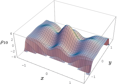
a)

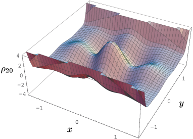
b)

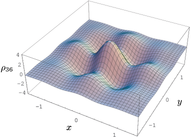
c)

FIG. 1.: The real part of the Taylor polynomial $\rho_{N}$ of the density matrix for a) $N=10$ b) $N=20$ and c) $N=36$. It is seen that the density matrix is retrieved for increasing values of the offdiagonal variable as the number of discrete time values are increased. $\rho_{36}$ is almost indistinguishable from the exact density matrix within the chosen plotting region.

The expansion (4) of the density matrix in terms of quasi-hydrodynamical moments can be generalized to systems with a higher number of dimensions. However, it may not be straightforward to generalize the recursion algorithm (17). This is basically due to the fact that the current density is not uniquely determined from the time derivative of the probability density for systems with two or more dimensions.

In conclusion, a method was found for reconstructing the density matrix of a particle in an arbitrary, time-dependent potential. The method was based upon a Taylor expansion of the density matrix in the off-diagonal variable. The coefficients $f_{n}$ in this expansion are hydrodynamical moments of the Wigner distribution. A recursive algorithm was found for calculating an arbitrary moment $f_{n}$ from the zeroth order moment, the probability distribution. In general, an $n$-th order Taylor polynomial of the density matrix can be found by observing the probability distribution at $n+1$ discrete time values.

REFERENCES

- [1] W. H. Zurek, Physics Today 44, 36 (1991).
- [2] E. Madelung, Z. Phys. 40, 322 (1926).
- [3] W. Gale, E. Guth, and G. T. Trammell, Phys. Rev. 165, 1434 (1968). D. I. Blokhintsev, The Philosophy of Quantum Mechanics (D. Reidel Publishing Company, Dordrecht, Holland, 1968). For a critical discussion on the completeness of the information contained in the probability density and the probability current density, see S. Weigert, Phys. Rev. A 53, 2078 (1996).
- [4] D. Hilbert, Matematische Annalen 72, 562 (1912).
- [5] G. E. Uhlenbeck and G. W. Ford, in Lectures in Statistical Mechanics (American Mathematical Society, Rhode Island, 1963), pp. 110–111.
- [6] E. Wigner, Phys. Rev. 40, 749 (1932).
- [7] P. Carruthers and F. Zachariasen, Rev. Mod. Phys. 55, 245 (1983).
- [8] J. E. Moyal, Proc. Cambridge Philos. Soc. 45, 99 (1949).
- [9] J. Yvon, J. de Phys. Lettr. 39, L363 (1978).
- [10] M. Ploszajczak and M. J. Rhoades-Brown, Phys. Rev. Lett. 55, 147 (1985). M. Ploszajczak and M. J. Rhoades-Brown, Phys. Rev. D 33, 3686 (1986).
- [11] J. V. Lill, M. I. Haftel, and G. H. Herling, Phys. Rev. A 39, 5832 (1989). J. V. Lill, M. I. Haftel, and G. H. Herling, J. Chem. Phys. 90, 4940 (1989).
- [12] H. M. Nussenzweig, Introduction to Quantum Optics (Gordon & Breach Science Publishers, London, 1973). W. Band and J. L. Park, Am. J. Phys. 47, 188 (1979).
- [13] A. Wünsche, Quantum Opt. 2, 453 (1990). C. T. Lee, Phys. Rev. A 46, 6097 (1992).
- [14] T. Richter, Phys. Rev. A 53, 1197 (1996). A. Wünsche, Phys. Rev. A 54, 5291 (1996).
- [15] U. Herzog, Phys. Rev. A 53, 2889 (1996).
- [16] J. Bertrand and P. Bertrand, Found. Phys. 17, 397 (1987).
- [17] K. Vogel and H. Risken, Phys. Rev. A 40, 2487 (1989).
- [18] D. Smithey, M. Beck, M. Raymer, and A. Faridani, Phys. Rev. Lett. 70, 1244 (1993). G. Breitenbach, S. Schiller, and J. Mlynek, Nature 387, 471 (1997).
- [19] C. Kurtsiefer, T. Pfau, and J. Mlynek, Nature 386, 150 (1997).
- [20] M. G. Raymer, M. Beck, and D. F. McAlister, Phys. Rev. Lett. 72, 1137 (1994).
- [21] U. Leonhardt and M. G. Raymer, Phys. Rev. Lett. 76, 1985 (1996).
- [22] S. Wallentowitz and W. Vogel, Phys. Rev. A 53, 4528 (1996). K. Banaszek and K. Wódkiewicz, Phys. Rev. Lett. 76, 4344 (1996).
- [23] D. Leibfried et al., Phys. Rev. Lett. 77, 4281 (1996).
- [24] For a survey, see the special issue Quantum State Preparation and Measurement, J. Mod. Opt. 44, No. 11/12 (1997)
- [25] T. Opatrny, D.-G. Welsch, and W. Vogel, Phys. Rev. A 56, 1788 (1997).
- [26] U. Leonhardt, Phys. Rev. A 55, 3164 (1997).
- [27] L. M. Johansen, electronic preprint quant-ph/9804002. To appear in proceedings of the Fifth International Conference on Squeezed States and Uncertainty Relations.
- [28] A. Royer, Found. Phys. 19, 3 (1989).
- [29] It can be noted that the recursion relations (17) coincide with the corresponding classical relations obtained from the classical Liouville distribution provided that the potential is a polynomial of maximally second order in . Moreover, the recursion relations for (giving , and ) coincide with the classical ones regardless of potential.