Optical Tachyons in Parametric Amplifiers: How Fast Can Quantum Information Travel?

Abstract

We show that optical tachyonic dispersion corresponding to superluminal (faster than-light) group velocities characterizes parametrically amplifying media. The turn-on of parametric amplification in finite media, followed by illumination by spectrally narrow probe wavepackets, can give rise to transient tachyonic wavepackets. In the stable (sub-threshold) operating regime of an optical phase conjugator it is possible to transmit probe pulses with a superluminally advanced peak, whereas conjugate reflection is always subluminal. In the unstable (above-threshold) regime, superluminal response occurs both in reflection and in transmission, at times preceding the onset of exponential growth due to the instability. Remarkably, the quantum information transmitted by probe or conjugate pulses, albeit causal, is confined to times corresponding to superluminal velocities. These phenomena are explicitly analyzed for four-wave mixing, stimulated Raman scattering and parametric downconversion.

I Introduction

A variety of mechanisms is now known to give rise to superluminal (faster-than-$c$) group velocities, which express the peak advancement of electromagnetic pulses reshaped by material media:

1. Near-resonant absorption[1, 2]: anomalous dispersion in the linear regime of an absorbing medium forms the basis for this superluminal reshaping mechanism.

2. Reduced transmission or evanescent wave formation (tunneling) in passive dielectric structures[3, 4, 5]: this reshaping mechanism has been attributed to interference between multiply-reflected propagating pulse components in the structure[6].

3. Soliton propagation in dissipative nonlinear structures [7]: superluminal group velocities can occur in such systems via nonlinear three-wave exchanges, as in stimulated Brillouin backscattering in the presence of dissipation. They also occur in a nonlinear laser amplifier[8].

4. Pulse propagation in transparent (non-resonant) amplifying media[9, 10]. Superluminal pulse reshaping in this regime has been attributed to either the dispersion[9] or the boundary reflections[10] of the amplifying medium.

5. Tachyonic dispersion in inverted two-level media: the dispersion in such inverted collective systems is analogous to the tachyonic dispersion exhibited by a Klein-Gordon particle with imaginary mass[11]. Consequently, it has been suggested [12] that probe pulses in such media can exhibit superluminal group velocities provided they are spectrally narrow. Gain and loss have been assumed to be detrimental for such reshaping. We note that Ref. [12] describes an infinite medium and boundary effects on the reshaping have not been considered.

While Ref. [12] suggests that tachyonic semiclassical propagation is measurable in optics, it provokes several important questions: (i) What other optical processes can give rise to tachyonic behavior, and under what conditions? (ii) What is the fundamental origin of tachyonic dispersion, and does it require optical coherence? This question is prompted by our earlier finding [6] that coherence is the key to superluminal group velocity of evanescent EM wavepackets (photon tunneling) in linear dielectric media [3, 4, 5]. (iii) Most intriguingly, is it possible to generate tachyon quanta and thereby transmit information without causality violation? The subtlety of this question is underscored by the following consideration: If a single-photon input could be transformed by a medium of length $L$ into a tachyonic quantum, whose detection probability is localized at times shorter than $L/c$, then such detection would provide information superluminally (!).

Our search for answers to these questions has resulted in the present theory [13], which reveals the conditions for the observability of EM wavepackets with tachyonic features in any parametrically amplifying (PA) medium. These conditions are explicitly analyzed for processes such as stimulated Raman scattering (SRS), parametric downconversion (PDC) and optical phase conjugation (OPC). Two remarkable findings emerge from the present analysis, which employs a new measure of wavepacket reshaping, namely, its time-dependent quantum information (change in Shannon entropy): (1) Tachyonic wavepackets transmit much less quantum information per photon than the probe wavepackets, and their temporal resolution is much worse than $L/c$, in accordance with causality. However, their information content is confined to superluminally short times, well below $L/c$. This finding may lead to the application of tachyonic propagation in communications. (2) Unlike evanescent EM wavepackets in linear dielectric media, tachyonic wavepackets are insensitive to decoherence.

II Tachyonic Dispersion in Infinite PA Media

Our analysis will disclose the role of spatial and temporal boundary conditions on tachyonic propagation in PA media. To this end, let us first review the properties of an infinite, one dimensional (1D) PA medium:

(a) The simplest model consists of two parametrically-coupled fields at different (nondegenerate) frequency bands, denoted by mode operators $\{a_{\vec{k}}\}$ and $\{b_{\vec{k}}\}$ . If their coupling is effected by a classical pump field at frequency $\omega_{0}$, then their interaction Hamiltonian is energy nonconserving,

$$H_{\text{int}}=-i\hbar\sum_{k\,k^{\prime}}(g_{k\,k^{\prime}}a_{k}b_{k^{\prime}}e^{i\omega_{0}t}-{\mbox{h}.c.}).$$

It describes two-photon creation or annihilation in correlated (“signal” and “idler”) modes, at the expense of the classical (undepleted) pump field, whose amplitude determines the coupling $g_{k\,k^{\prime}}$. When the following conditions hold: (i) the $k$-dependence (dispersion) of $g_{k\,k^{\prime}}$ is negligible, $g_{kk^{\prime}}\rightarrow g$; (ii) phase matching prevails, and (iii) the uncoupled frequencies are $\omega_{a(b)\,k}\simeq\omega_{0}\pm c(k-k_{0})$, we can diagonalize this hamiltonian in the interaction picture (upon transforming away the $\omega_{0}$- and $k_{0}$-dependence) by the Bogoliubov transformation (BT)

$$D {}_{k}=u_{k}a_{k}+v_{k}b^{+}_{-k},\quad[D_{k},H]=\hbar\omega_{k}D_{k},$$ (1)

$$u {}_{k}=\sinh{s_{k}},\quad v_{k}=e^{i\phi}\cosh{s_{k}},\quad\tanh^{2}{s_{k}}=|g|^{2}/|\omega_{k}+ck|^{2}.$$ (2)

Whereas the significance of $s_{k}$ as the squeezing parameter is well known [14], much less attention has been paid [15] to the dispersion relation obtainable from eqs.(1-2) (Fig. 1)

$$\omega_{k}=\pm\sqrt{(ck)^{2}-|g|^{2}}$$ (3)

which is tachyonic, i.e., isomorphic to that of a Klein-Gordon particle with imaginary mass [12, 16], and yields superluminal group velocities $|d\omega_{k}/dk|\geq c$ for spectrally narrow photonic wavepackets.

FIG. 1.: Dispersion relation (solid line) in a OPC. The dashed (dotted) lines correspond to the dispersion relation for the probe (p) and conjugate (c) waves in vacuum and $k_{0}\equiv\omega_{0}/c$.

(b) This behavior should be contrasted with that obtained when we replace the parametric-coupling by the energy-conserving

$$H_{\text{int}}=i\hbar g\sum_{k}(a_{k}b_{k}^{+}-\mbox{h.c.}).$$

This model pertains to light scattering in passive, non-dissipative media, e.g., periodic dielectric structures with two-band dispersion. The diagonalizing BT in this case describes passive light reflection

$$D_{k}=u_{k}a_{k}+v_{k}b_{-k}\,\text{ with }\,u_{k}=\sin{\theta_{k}},\;v_{k}=e^{i\phi}\cos{\theta_{k}}\,\text{ and }\,\tan^{2}{\theta_{k}}=|g|^{2}/|\omega_{k}+ck|^{2}.$$

This BT yields the polaritonic dispersion

$$\omega_{k}=\pm\sqrt{(ck)^{2}+|g|^{2}}$$ (4)

which is analogous to that of Klein-Gordon particles with real masses (“bradyons”) and allows only subluminal group velocities $|d\omega/dk|\leq c$.

A more general model of infinite PA media accounts for both energy conserving and nonconserving exchanges, and therefore pertains to a wider range of optical parametric processes

$$H = \sum_{j^{\prime},j=\pm,k>0}\{\hbar ck(a_{jk}^{+}a_{jk}+\frac{1}{2})+\hbar\Omega_{k}(b_{jk}^{+}b_{jk}+\frac{1}{2})$$ (5)

$$+ i\hbar g_{k}[(a_{jk}^{+}b_{jk}-\mbox{h.c.})+(a_{jk}b_{j^{\prime}k}-\mbox{h.c.})]\}$$ (6)

When this 4-mode coupling Hamiltonian is diagonalized by means of a BT, it yields a 4-branch dispersion, with two polaritonic and two tachyonic branches. In the nondispersive limit $\Omega_{k}\rightarrow\Omega_{0}$, this model pertains to SRS with Stokes and anti-Stokes scattering corresponding to the energy-conserving and non-conserving terms in eq.(5). The distance between the Stokes and anti-Stokes pairs of branches is determined by $\Omega_{0}$, whereas each pair is split by $g$ (Fig. 2). Strong non-degeneracy of the two pairs of branches $\Omega_{0}>g$ is required to separate between tachyonic and bradyonic (polaritonic) types of dispersion (described by eqs.(3) and (4)). Otherwise, hybrid (mixed tachyon-bradyon) branches can arise. When strong non-degeneracy exists, the tachyonic branches in Fig. 2 are rotated by 45^∘ relative to those corresponding to eq.(3) and are isomorphic to their tachyonic counterparts in the inverted two-level model [12].

FIG. 2.: SRS dispersion obtained from a sum of the energy-conserving and nonconserving two-mode hamiltonians discussed in text. Upper curves – Stokes dispersion (tachyonic), lower curves – anti-Stokes dispersion (bradyonic or tardyonic).

The observability of the above tachyonic dispersion poses not only the unrealistic requirement that the PA medium be infinite, but also that we detect the field “dressed” by the medium, obeying eqs. (1-3) (or their equivalent for eq. (5)), rather than the “bare” field (unperturbed by $H_{int}$). If the PA coupling is turned on at $t=0$ throughout a very long medium, then a probe wavepacket in a multimode (Gaussian-distributed) state will be reshaped at $t>0$ in the dressed-field basis to exhibit superluminal peak advancement, without any gross distortion. However, it will be accompanied by broadband excitation of quanta arising from vacuum fluctuations within the phase-matched spectral band, with relative weights $\langle D^{+}_{k}D_{k}\rangle=\cosh^{2}s_{k}$. In the bare-field basis, the reshaping of the probe wavepacket at $t>0$ will be more complicated, and eventually result in its exponential growth.

III Quantum Description of finite OPC

In the rest of the paper, the above reshaping and dispersion will be compared with those of probe photons injected into finite PA media of length $L$. We shall adopt a one-dimensional description of propagation, consistently with the standard paraxial approximation. Since we wish to explore time-resolved information transfer, the first generic regime to be addressed is that of abruptly switched-on pump fields and short (transient) wavepacket transmission times $L/c\lesssim t\ll\tau_{\text{rel}}$, where $\tau_{\text{rel}}$ is the medium relaxation (or dissipation) time. Superluminal features in this regime require the simultaneous pumping of the entire medium, otherwise pump retardation dictates the probe propagation velocity. Simultaneous pumping of the medium is possible in OPC, where pump pulses can be perpendicular to the medium axis $z$ (Fig. 3-inset).

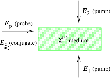
FIG. 3.: Conjugate (reflected) wavepacket reshaping in OPC: dependence of flux $\langle n_{c}\rangle$ (in units $c/L$) at $z=0$ on time (for $|g|L=1.7$, probe width (FWHM for Gaussian amplitude) $\Delta_{t}=24L/c$, probe detuning from PA resonance $\delta=0.28c/L$, $t_{p}=50L/c$, $\langle N_{p}\rangle=10^{10}$); 1 – Gaussian probe transmitted in empty space; 2 – corresponding conjugate $\langle n_{c}^{(resp)}\rangle$: observe the superluminally advanced peak at $t\simeq 42L/c$, followed by exponential growth (instability) at $t\gtrsim 50L/c$; 3 – exponentially-growing “noise” $\langle n_{c}^{(sp)}\rangle$; 4 – abruptly switched-on probe (onset at $10L/c$, delay $t_{p}=20L/c$), 5 – exponentially-growing conjugate corresponding to the latter.

The quantized analysis of OPC following the abrupt turn-on of the pump throughout the medium has been undertaken by us for the first time. It amounts to solving the coupled-wave equations for the slowly varying probe ($p$) and conjugate ($c$) field operators $\hat{E}_{p(c)}^{(\pm)}(z,t)$,

$$\frac{\partial\hat{E}_{p}^{(-)}}{\partial z}+\frac{1}{c}\frac{\partial\hat{E}_{p}^{(-)}}{\partial t}=ig^{*}\hat{E}_{c}^{(+)},$$ (7)

$$\frac{\partial\hat{E}_{c}^{(+)}}{\partial z}-\frac{1}{c}\frac{\partial\hat{E}_{c}^{(+)}}{\partial t}=ig\hat{E}_{p}^{(-)}.$$ (8)

Here the coupling constant $g$ is proportional to the pump intensity, which is assumed to be turned on at $t=0$. The non-standard source terms, i.e., $\hat{E}_{p}^{(-)}(z,t=0)$ and $\hat{E}_{c}^{(+)}(z,t=0)$, account for the initial ($t=0$) vacuum fluctuations of the probe and conjugate fields, respectively, at any point $z$ of the medium ($0\leq z\leq L$). Additional sources of vacuum fluctuations are the input fields $\hat{E}_{p}(z=0,t)$ and $\hat{E}_{c}(z=L,t)$ at the forward and rear faces of the medium, respectively, which are taken to be in the vacuum state. The nonvanishing correlation functions of the source terms can be concisely expressed as

$$\langle\hat{E}_{p(c)}^{(+)}(z,t)\hat{E}_{p(c)}^{(-)}(z^{\prime},t^{\prime})\rangle_{\text{vac}}=A\delta(z-z^{\prime}\mp c(t-t^{\prime})),$$ (9)

where the upper (lower) sign refers to the probe (conjugate) field, and $A=\hbar\omega_{0}k_{0}^{2}\Omega/2\pi$, $\Omega$ being the solid angle in which the output is detected.

We have solved Eqs. (8), taking account of Eq. (9), to allow for spontaneous parametric generation of both probe and conjugate fields from vacuum fluctuations, along with response to an injected probe field $\epsilon_{p}f_{p}(t)$. Specifically $|f_{p}(t)|$ will be a bell-shaped function with the maximum at $t_{0}$ satisfying $|f_{p}(t)|\leq|f_{p}(t_{0})|=1$. The average conjugate-reflected flux (photons/sec) through the cross-section ${\cal S}$ and solid angle $\Omega$ at $z=0$ is the sum of the two above components, $\langle n_{c}\rangle=\langle n_{c}^{(sp)}\rangle+\langle n_{c}^{(resp)}\rangle$,

$$\langle n_{c}^{(sp)}(z=0,t)\rangle=\kappa^{2}\alpha\frac{c}{L}\left[\int_{0}^{1}G_{p}^{2}(\zeta,\tau)d\zeta+\int_{0}^{\tau}G_{p}^{2}(0,\tau^{\prime})d\tau^{\prime}\right],$$ (11)

$$\langle n_{c}^{(resp)}(z=0,t)\rangle=\kappa^{2}\alpha\langle n_{p}\rangle\left|\int_{0}^{\tau}G_{p}(0,\tau-\tau^{\prime})f_{p}(\tau^{\prime})d\tau^{\prime}\right|^{2},$$ (12)

where $\kappa=|g|L$ is the dimensionless coupling strength, $\alpha=\Omega S/\lambda_{0}^{2}$, $\lambda_{0}$ is the pump wavelength, $\zeta=z/L,\ \tau=ct/L$, and $\langle n_{p}\rangle$ is the maximum probe flux, $\langle n_{p}\rangle=\langle N_{p}\rangle/\int_{-\infty}^{\infty}|f_{p}(t)|^{2}dt$, $N_{p}$ being the number of photons in the probe pulse which pass through ${\cal S}$ into the solid angle $\Omega$. Solution (3) is expressed in terms of the Green function (App.A)

$$G_{p}(\zeta,\tau)=\frac{1}{2}\sum_{j=0}^{\infty}\left\{\left[\left(\frac{\tau-\tau_{j}^{+}}{\tau+\tau_{j}^{+}}\right)^{j}I_{2j}\left(\kappa\sqrt{\tau-\tau_{j}^{+}}\right)\right.\right.$$ (13)

$$\left.\left.-\left(\frac{\tau-\tau_{j}^{+}}{\tau+\tau_{j}^{+}}\right)^{j+1}I_{2j+2}\left(\kappa\sqrt{\tau-\tau_{j}^{+}}\right)\right]\theta(\tau-\tau_{j}^{+})-(\tau_{j}^{+}\rightarrow\tau_{j}^{-})\right\}.$$ (14)

Here $\tau_{j}^{+}=2j+\zeta$ and $\tau_{j}^{-}=2(j+1)-\zeta$ are, respectively, the forward- and backward-propagation retardation times after $j$ round trips, $I_{2j}()$ stands for the modified Bessel function of $2j$-th order, and $\theta()$ for the Heaviside step function.

The first term in $\langle n_{c}^{(sp)}(t)\rangle$, Eq.(11), is the response to the initial ($t=0$) vacuum fluctuations of the probe. The second term therein represents the response to the probe vacuum fluctuations (taking them as $\delta$-correlated) at the input (forward) face $z=0$. The phase-conjugate response $\langle n_{c}^{(resp)}\rangle$ (Eq.(12)) to the incident probe photon flux is identical with the classical response to the same probe intensity and pulse shape $f_{p}(t)$. The Green function in (14) ensures causality by the step functions $\theta(\tau-\tau_{j}^{\pm})$. These step functions imply that the $j=0$ term of the response allows superluminal reshaping only via the forward tail of the probe wavepacket extending throughout the medium at $t=0$. The $j\neq 0$ terms in (14) account for multiple reflections at the boundaries.

Above the threshold for parametric instability, the spontaneous parametric radiation $\langle n^{(sp)}_{c}(t)\rangle$ (triggered by the probe vacuum fluctuations) grows at $t>0$ nearly exponentially. Nevertheless, there can be quasi-tachyonic reshaping, namely, the transformation of a Gaussian probe wavepacket into a wavepacket $\langle n_{c}^{(resp)}(t)\rangle$, which resembles a Gaussian with a superluminally advanced peak at times $0<t<t_{u}$. The time $t=t_{u}$ marks the end of quasi-tachyonic reshaping and the start of the unstable classical response, i.e., the onset of exponential growth of $\langle n_{c}^{(resp)}(t)\rangle$, so that at $t>t_{u}$ the output becomes unrelated to the input. This growth is changed at $t\gtrsim\tau_{\text{rel}}$, $\tau_{\text{rel}}$ being the relaxation time (see below). This sharp separation of the two evolution stages: $0<t<t_{u}$, the tachyon transient time, and the instability growth time $t_{u}<t<\tau_{\text{rel}}$ is contingent on the following conditions. We need a narrow spectral width of the incident probe, large detuning of the probe central frequency from parametric resonance, and large delay time $t_{p}$ between the pump turn-on $t=0$ and the arrival of the incident-probe peak at $z=0$, otherwise there is fast onset of the instability (Fig. 4).

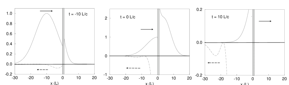
FIG. 4.: Unstable (above-threshold) regime of the OPC: reflection and transmission of an incoming probe pulse. The OPC medium is located between $0<x<L$ (see shaded area). The upper (lower) half of each time plot shows the probe (conjugate) pulse $|{\cal E}_{p}(x,t)|^{2}$ (- $|{\cal E}_{c}(x,t)|^{2}$), which is moving to the right (left). Parameters used are $\delta_{0}=0.31\,c/L$, $\Delta_{t}=19.3\,L/c$, $gL=1.7$.

IV Quantum Information Travel in OPC

What is the physical significance, if any, of the quasi-tachyonic reshaping at $0<t<t_{u}$? To answer this question, we have considered a quantity that has not been used before to study wavepacket reshaping, namely, the time-dependent quantum information function $\Delta H_{c}(t)$, associated with the Shannon entropy of the detected flux $\langle n_{c}(t)\rangle$. This function reads [17]

$$\Delta H(t) = \langle n_{c}\rangle\log_{2}\left(1+\frac{1}{\langle n_{c}\rangle}\right)$$ (15)

$$+ \log_{2}\left(1+\frac{\langle n_{c}^{(resp)}\rangle}{\langle n_{c}^{(sp)}\rangle}\right)-\langle n_{c}^{(sp)}\rangle\log_{2}\left(1+\frac{1}{\langle n_{c}^{(sp)}\rangle}\right)$$ (16)

A similar function $\Delta H_{p}(t)$ can be defined for the transmitted probe $\langle n_{p}(t)\rangle$. When the probe wavepacket envelope $f_{p}(t)$ has a sharp front, these information functions behave causally, i.e., they grow only at times satisfying retardation. However, when $f_{p}(t)$ has an extended forward tail, then these functions exhibit apparent superluminal advancement compared to the same function for a probe in free space (Fig. 5). The reason for this is that the forward tail of the probe is transformed into $\langle n_{c}^{(resp)}\rangle$ right after the pump turn-on at $t=0$, hence this information growth is due to the nonlocal (simultaneous) pump effect throughout the medium, and no retardation is expected. The information increases until $\langle n_{c}^{(sp)}\rangle$, which grows exponentially and contributes negatively to $\Delta H$, becomes appreciable, compared to $\langle n_{c}^{(resp)}\rangle$. This causes $\Delta H_{c}$ to be confined to earlier times than the peak of $\langle n_{c}(t)\rangle$!

FIG. 5.: Information transfer $\Delta H_{c}$ (Eq.(16)), same parameters as in Fig. 3, except for $\langle N_{p}\rangle=100$; A – for Gaussian probe in empty space $\Delta H_{c}$ follows probe shape; B – for corresponding conjugate (with “noise”), $\Delta H_{c}$ is peaked at an earlier time $t\simeq 30L/c$, than curve 2 in Fig. 3, but is $10^{6}$ times smaller; C – for chopped probe (onset at $10L/c$) transmitted through empty space; D – for conjugate (with “noise”) corresponding to the latter, note that $\Delta H_{c}$ is no longer advanced, but peaked at $t\simeq 20L/c$, just as curve C.

Note, however, that the total amount of information transfer is sharply reduced as compared to that of a probe in free space, and does not exceed that of the front tail of the free-space probe, as required by causality. Nevertheless, the temporal compression of the information due to the nonlocal character of the response is a potentially useful novel feature for communications: it indicates the appropriate time intervals for modulation of the probe envelope, so as to optimize the information transfer. As seen from Fig. 5 the Gaussian probe envelope can be switched off well before it reaches its peak, since the transferred information $\Delta H_{c}$ is derived only from the forward tail! Likewise, the minimal useful interval between successive probe peaks should exceed the temporal width of $\Delta H_{c}$.

V Tachyonic Propagation in SRS

In SRS, by contrast to OPC, the pump cannot be switched on simultaneously throughout the sample rather the pump is moving along the sample (in the $z$ direction) with a front velocity $c$. Therefore the Stokes (signal) field in SRS or signal in PDC has superluminal features only if the pump front sweeps the sample axis $z$ at a speed exceeding $c$, as allowed by the experimentally feasible “searchlight effect”.

On the other hand, the SRS regime in which superluminal features are displayed even for a stationary pump is that of long times, at which transient effects due to the pump turn-on play no role already, but relaxation effects are no longer negligible. The slowly varying Stokes field operator in SRS for a stationary laser pump intensity $I_{L}$, and relaxation (dissipation) rate $\Gamma=1/\tau_{\text{rel}}$, is given by the known solution [18]

$$\hat{E}_{s}^{(-)}(z,t)=\hat{E}_{s}^{(-)}(0,t)+\frac{1}{2}\alpha^{1/2}\left\{z^{1/2}\int_{0}^{t}dt^{\prime}e^{-\Gamma t^{\prime}}\frac{I_{1}[(\alpha zt^{\prime})^{1/2}]}{(I_{L}t^{\prime})^{1/2}}\hat{E}_{s}^{(-)}(0,t-t^{\prime})\right.$$ (17)

$$\left.-ie^{-\Gamma t}\int_{0}^{z}dz^{\prime}\hat{Q}^{\dagger}(z-z^{\prime},0)I_{0}[(\alpha z^{\prime}t)^{1/2}]-i\int_{0}^{t}dt^{\prime}\int_{0}^{z}dz^{\prime}e^{-\Gamma t^{\prime}}I_{0}[(\alpha z^{\prime}t^{\prime})^{1/2}]\hat{F}^{\dagger}(z^{\prime},t^{\prime})\right\}.$$ (18)

Here $\alpha=g\Gamma=4\kappa^{2}I_{L}$, $\hat{F}(z,t)$ is the $\delta$-correlated (in space and time) Langevin operator describing the field dissipative fluctuations, and $\hat{Q}(z,0)$ is the initial spatially $\delta$-correlated atomic inversion operator.

The plots (Fig. 6) show the output Stokes (signal) of the average intensity $\langle n_{s}\rangle=\langle\hat{E}_{s}^{(-)}(z,t)\hat{E}_{s}^{(+)}(z,t)\rangle$ obtainable from (18) for incident Gaussian input wavepackets with appropriately chosen width, mean frequency and peak delay (after the pump turn-on at $t=0$), reveal a surprising finding: quasi-tachyonic reshaping obtains for large transit times $t\gg\tau_{\text{rel}}$ (if the response contribution to $\langle n_{s}\rangle$ strongly exceeds the vacuum fluctuations contribution, which comes from the last two terms in (18)). This reshaping is essentially similar to that of the transient ($t\ll\tau_{\text{rel}}$) regime of OPC (Fig. 3). Hence, relaxation (and the resulting destruction of temporal coherence) does not preclude the tachyonic reshaping, as opposed to the superluminal reshaping of optical evanescent waves, which is essentially a coherent (interference) process [6]. Here, by contrast, tachyonic reshaping in the presence of dissipation originates from the $t^{\prime}$-dependence of the integrand $e^{-\Gamma t^{\prime}}I_{1}[(\alpha zt^{\prime})^{1/2}]/\sqrt{t^{\prime}}$ in (18), which is similar to that of a Gaussian (spectrally dispersive) function. This conclusion can be generalized to any PA medium: for $t\gg\tau_{\text{rel}}$, it is possible to observe tachyonic dispersion by taking advantage of the high spectral selectivity of the parametric gain coefficient, $\sim g/[1+\tau_{\text{rel}}(\omega-\omega_{0})]$, which is limited to a band of width $\sim\Gamma=1/\tau_{\text{rel}}$. After the pump is switched on, at times $t\gtrsim\tau_{\mbox{rel}}$, the Fourier-transformed response function has the generic form $\tilde{G}(\delta)\simeq e^{\frac{(gL/c)}{1+(\tau_{\text{rel}}\delta)^{2}}}\simeq e^{\frac{gL}{c}(1-(\tau_{\text{rel}}\delta)^{2})}$, where $\delta=\omega-\omega_{0}$. The nearly-Gaussian shape of the response $\tilde{G}(\delta)$ allows for tachyonic features, when $\tilde{G}(\delta)$ is convoluted with a Gaussian probe.

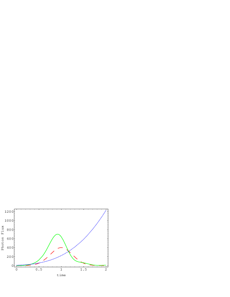
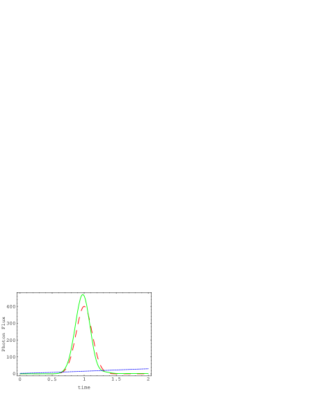
FIG. 6.: Transmitted SRS photon flux ($\langle n_{s}\rangle/\Gamma$) as a function of time ($\Gamma t$): dotted line – exponentially-growing spontaneous (vacuum fluctuations) “noise”; dashed line – the probe flux in free space; solid line – induced response with superluminally-advanced peak compared to dashed line. (a) Detuning $\delta/\Gamma=10$, probe pulse width $\Delta/\Gamma=0.5$, $gL=25$; (b) detuning $\delta/\Gamma=15$, probe pulse width $\Delta/\Gamma=0.25$, $gL=12$.

VI Conclusions

Our theory has yielded the following conclusions, which elucidate the nature and observability of tachyon effects in quantized PAs: (a) Tachyons are the characteristic quanta generated in any infinite parametrically amplifying (PA) medium, involving processes such as stimulated Raman scattering (SRS), parametric down conversion (PDC) and optical phase conjugation (OPC). The basic connection between parametrically amplifying (PA) processes and tachyonic dispersion is that their inherent energy-nonconservation entails lack of symmetry under time reversal, along with translational invariance (momentum conservation or phase matching). This signifies that the space and time (or energy and momentum) axes in PA dispersion are interchanged as compared to the energy-conserving, time-reversible polaritonic dispersion, corresponding to the 90^∘ rotation of axes when passing from a bradyonic Lorentz transformation to the tachyonic generalized Lorentz transformation [19]. (b) In a PA medium of length $L$, only probe wavepackets with macroscopic photon numbers and temporal width well above $L/c$ can be reshaped into observable (transmitted or reflected) tachyonic wavepackets (characterized by superluminal peak advancement and little distortion). The observability of these tachyonic wavepackets is limited to transient times by the inherent quantum instability of PA processes, i.e., the broadband amplification of vacuum fluctuations on the one hand, and, on the other hand, by the classical instability (exponential growth) associated with gain. (c) As a result of competition between reshaping and instability the information content of tachyonic wavepackets is confined to times well below $L/c$, although causality is not violated. This novel feature is shown to be advantageous for communications. (d) Tachyonic dispersion of probe wavepackets is observable even in the dissipative, incoherent propagation regime, by virtue of the PA gain dispersion in the presence of dissipation.

We acknowledge useful discussions with I. Bialinicki-Birula and Y. Silberberg, and the support of Minerva and EU(TMR) grants.

A The Green function derivation for OPC

In this appendix we briefly outline the two-sided Laplace transform (TSLT) technique introduced by Fisher et al.[20] for the derivation of Green function. The TSLT is defined as $\tilde{\cal F}_{(*)}(x,s)\equiv\int_{-\infty}^{\infty}dt\,F^{(*)}(x,t)\,e^{-st}$. It is only valid for functions $F(x,t)$ that diminish faster than exponentially at times $t\to-\infty$. Its advantage compared to the the usual one-sided Laplace transform is that it also applies to functions that do not vanish at $t<0$. The starting point of the analysis is to apply the TSLT to the four-wave mixing equations (8) with $F(x,t)={\cal E}_{p}(x,t)$ or ${\cal E}_{c}^{*}(x,t)$. We then obtain the coupled equations

$$\left\{\begin{array}[]{l}\frac{d}{dx}\,\tilde{\cal E}_{p}(x,s)+\frac{s}{c}\,\tilde{\cal E}_{p}(x,s)+ig\,\tilde{\cal E}_{c,*}(x,s)=0\vspace{0.3cm}\\ \frac{d}{dx}\,\tilde{\cal E}_{c,*}(x,s)-\frac{s}{c}\,\tilde{\cal E}_{c,*}(x,s)+ig^{*}\,\tilde{\cal E}_{p}(x,s)=0.\end{array}\right.$$ (A1)

Equations (A1) are solved together with the Laplace transforms of the boundary conditions ${\cal E}_{p}(0,t)=F(0,t)$, where $F(0,t)$ is an incident probe pulse at the entry $x=0$ of the PCM medium, and ${\cal E}_{c}(L,t)=0$, so no incoming conjugate pulse at the end of the medium. The result is

$$\tilde{\cal E}_{c}(x,s) = h_{r}(x,is)\,\tilde{\cal F}_{*}(0,s)$$ (A2)

$$\tilde{\cal E}_{p}(x,s) = h_{t}(x,is)\,\tilde{\cal F}(0,s),$$ (A3)

with the reflection and transmission amplitudes

$$h_{r}(x,\delta) = \frac{|g|\sin(\beta(L-x))}{\frac{\delta}{c}\mbox{\rm sin}(\beta L)+i\beta\mbox{\rm cos}(\beta L)}\vspace{0.3cm}$$ (A4)

$$h_{t}(x,\delta) = \frac{i\beta\cos(\beta(L-x))+\frac{\delta}{c}\sin(\beta(L-x))}{\frac{\delta}{c}\mbox{\rm sin}(\beta L)+i\beta\mbox{\rm cos}(\beta L)},$$ (A5)

where

$$\beta=\frac{1}{c}\sqrt{\delta^{2}+|gc|^{2}}.$$ (A6)

The reflected phase-conjugate pulse ${\cal E}_{c}(x,t)$ and transmitted probe pulse ${\cal E}_{p}(x,t)$ at position $x$ in the nonlinear medium and time $t$ are then obtained by using the inverse Laplace transform. At $x=0$ and $x=L$, respectively, they are given by

$${\cal E}_{c}(0,t) = \frac{1}{2\pi i}\int_{\gamma-i\infty}^{\gamma+i\infty}ds\,r_{cp}(is)\,\tilde{{\cal E}}_{p^{*}}(0,s)\,e^{st}$$ (A7)

$${\cal E}_{p}(L,t) = \frac{1}{2\pi i}\int_{\gamma-i\infty}^{\gamma+i\infty}ds\,t_{pp}(is)\,\tilde{{\cal E}}_{p}(0,s)\,e^{st},$$ (A8)

where $r_{cp}=h_{r}(x=0)$ and $t_{pp}=h_{t}(x=L)$. The choice of contour $\gamma$ is in agreement with causality, which means in this case that it is to the right of all the singularities of $r_{cp}(is)$ (and $t_{pp}(is)$). The singularities in the right-half s-plane give rise to exponential growth of ${\cal E}_{c}(x,t)$ and ${\cal E}_{p}(x,t)$. The integrals (A7) and (A8) can be evaluated by taking the contribution of these poles separately and rewriting the remaining integral as a Fourier integral.

They can also be evaluated in another way, which is especially insightful when regarding non-analytic, chopped probe pulses. To that end we rewrite (A7) and (A8) as

$${\cal E}_{c}(0,t) = \int dt^{{}^{\prime}}\,{\cal E}_{p}^{*}(0,t^{{}^{\prime}})H_{c}(t,t^{{}^{\prime}})$$ (A9)

$${\cal E}_{p}(L,t) = \int dt^{{}^{\prime}}\,{\cal E}_{p}(0,t^{{}^{\prime}})H_{p}(t,t^{{}^{\prime}}),$$ (A10)

with

$$H_{c}(t,t^{{}^{\prime}}) = \frac{1}{2\pi i}\int_{\gamma-i\infty}^{\gamma+i\infty}ds\,r_{cp}(is)\,e^{-s(t^{{}^{\prime}}-t)}$$ (A11)

$$H_{p}(t,t^{{}^{\prime}}) = \frac{1}{2\pi i}\int_{\gamma-i\infty}^{\gamma+i\infty}ds\,t_{pp}(is)\,e^{-s(t^{{}^{\prime}}-t)}$$ (A12)

In order to evaluate the integral in, e.g., $H_{p}(t,t^{{}^{\prime}})$, $t_{pp}$ is first rewritten as the series

$$t_{pp}(is)=2\eta\sum_{n=0}^{\infty}\frac{a^{2n}}{(s+\eta)^{2n+1}}\,e^{-(n+\frac{1}{2})\eta\tau}$$ (A13)

with $a\equiv\kappa_{0}c$, $\eta\equiv\sqrt{s^{2}-a^{2}}$ and $\tau=2L/c$, the roundtrip time of the PCM. One can then easily prove that (A13) is uniformly convergent, which allows for term by term integration of (A12). We use the substitution

$$s=\frac{ia}{2}\left(\frac{u}{A_{n}}-\frac{A_{n}}{u}\right)$$ (A14)

with

$$A_{n}\equiv\left(\frac{t-t^{{}^{\prime}}-(n+\frac{1}{2})\tau}{t-t^{{}^{\prime}}+(n+\frac{1}{2})\tau}\right)^{1/2},$$ (A15)

in which $t^{{}^{\prime}}+(n+\frac{1}{2})\tau$ is the retardation time after $(n+\frac{1}{2})$ round trips. We then arrive at the following form of the conjugate reflected pulse

$${\cal E}_{c}(L,t) = \int_{-\infty}^{t}dt^{{}^{\prime}}\,{\cal E}_{p}^{*}(0,t^{{}^{\prime}})\,G_{0}(t,t^{{}^{\prime}})+$$ (A17)

$$-2\sum_{n=1}^{\infty}\int_{-\infty}^{t-n\tau}dt^{{}^{\prime}}{\cal E}_{p}^{*}(0,t^{{}^{\prime}})\,G_{n}(t,t^{{}^{\prime}}),$$

with

$$\begin{array}[]{rl}G_{n}(t,t^{{}^{\prime}})&=\frac{-i\,\kappa_{0}c}{4}\left(B_{n}^{n-1}I_{2n-2}\left[|g|c\,\sqrt{(t-t^{{}^{\prime}})^{2}-n^{2}\tau^{2}}\,\right]\right.\vspace{0.2cm}\\ &-2B_{n}^{n}I_{2n}\left[|g|c\,\sqrt{(t-t^{{}^{\prime}})^{2}-n^{2}\tau^{2}}\,\right]\vspace{0.2cm}\\ &\left.+B_{n}^{n+1}I_{2n+2}\left[|g|c\,\sqrt{(t-t^{{}^{\prime}})^{2}-n^{2}\tau^{2}}\,\right]\ \ \right),\end{array}$$ (A18)

and

$$B_{n}\equiv\left(\frac{t-t^{{}^{\prime}}-n\,\tau}{t-t^{{}^{\prime}}+n\,\tau}\right).$$ (A19)

REFERENCES

- [1] L. Brillouin, Wave Propagation and Group Velocity, (Academic Press, New York, 1960).
- [2] C.G.B. Garrett and D.E. McCumber, Phys. Rev. A 1, 305 (1970); S. Chu and S. Wong, Phys. Rev. Lett. 48, 738 (1982).
- [3] M. Büttiker and R. Landauer, Phys. Rev. Lett. 49, 1739 (1982); Th. Martin and R. Landauer, Phys. Rev. A 45, 2611 (1992).
- [4] A. M. Steinberg, P.G. Kwiat, and R.Y. Chiao, Phys. Rev. Lett. 68, 2421 (1992).
- [5] A. Ranfagni, D. Mugnai, and A. Agresti, Phys. Lett. A 175, 334 (1993).
- [6] Y. Japha and G. Kurizki, Phys. Rev. A 53, 586 (1996).
- [7] E. Picholle, C. Montes, C. Leycuras, O. Legrand, and J. Botineau, Phys. Rev. Lett. 66, 1454 (1991).
- [8] A. Icsevgi and W.E. Lamb, Phys. Rev. 185, 517 (1969).
- [9] E. L. Bolda, Phys. Rev. A 54, 3514 (1996); E. L. Bolda, J.C. Garrison, and R.Y. Chiao, ibid 49, 2938 (1994).
- [10] M. Artoni and R. Loudon, Phys. Rev. A 57, 622 (1998).
- [11] Y. Aharonov, A. Komar, and L. Susskind, Phys. Rev. 182, 1400 (1969).
- [12] R.Y. Chiao, A.E. Kozhekin, and G. Kurizki, Phys. Rev. Lett. 77, 1254 (1996).
- [13] G. Kurizki, A. Kozhekin and A.G. Kofman, Europhysics Letters (in press); M. Blaauboer, A.E. Kozhekin, A.G. Kofman, G. Kurizki, D. Lenstra, and A. Lodder, Opt. Comm. 148, 295 (1998); M. Blaauboer, A.G. Kofman, A.E. Kozhekin, G. Kurizki, D. Lenstra, and A. Lodder, Phys. Rev. A. 57 (in press).
- [14] S.M.Barnett and P.L.Knight, J.Opt.Soc.Am.B 2, 467 (1985); C.M.Caves and B.L.Schumaker, Phys.Rev.A 31, 3068, 3093 (1985).
- [15] B.S. Wang and J.L. Birman, Phys.Rev.B 42, 9609 (1990) show numerically analogous features in the anomalous dispersion of phonoritons, namely, exciton-polaritons modified by the exciton-phonon interaction.
- [16] A.Yu. Andreev and D.A. Kirzhnits Sov.Phys.Uspekhi 39, 1071, (1996); D.A. Kirzhnits [Sov.Phys.Uspekhi] Usp.Fiz.Nauk 90, 129, (1966); P.Csonka, Nucl.Phys. B 21, 436 (1970); R.Fox, C.Kuper, S.Lipson, Proc.Roy.Soc. A 316, 515 (1970); Y.Aharonov et al., Phys.Rev. 182, 1400 (1969).
- [17] C.M. Caves and P. Drummond, Rev.Mod.Phys. 66, 481 (1994).
- [18] M.G. Raymer and J. Mostowski, Phys.Rev.A 24, 1980, (1981); M. G. Raymer, J. Mostowski, and J. L. Carlsten, Phys.Rev.A 19, 2304 (1979).
- [19] G. Feinberg, Phys.Rev. 159, 1089 (1967); O. Bilaniyk and E. Sudarshan, Phys.Today 22, 43 (1969); S. Weinberg, Phys.Rev.Lett. 19, 12260 (1967); R. Folman and E. Recami, Found.Phys.Lett. 8, 127 (1995); E. Recami, Rivista Nuovo Cim. 9, issue 6 (1986).
- [20] R.A. Fisher, B.R. Suydam, and B.J. Feldman, Phys. Rev A 23, 3071 (1981).